1. Introduction
Currently, electric vehicles represent a small fraction of the transportation sector. Nevertheless, different market analysts predict a high penetration of electric cars, which will increase up to 33% by 2040 [
1] and 50% by 2050 [
2]. The advancement propelling the increase in the penetration of electric vehicles is the battery, via both an increase in the energy density (kWh/kg) and a reduction in the cost per energy (USD/kWh). In 2018, costs were in the range of 209 USD/kWh [
3]. In 2020, the battery pack achieved a price of 137 USD/kWh [
4]. The International Renewable Energy Association (IRENA) anticipates a cost of 150 USD/kWh in the 2020s, which will make EVs a competitive transportation option [
5].
An electric vehicle needs to hold enough energy for the everyday commute and extra energy for extended travel. Charging technology is also relevant, since it is necessary to supply energy at a reasonable rate for the next day’s commute by charging at home and traveling beyond the battery charge capacity at public charging stations [
6]. The electrification of the transportation sector will lead to a reduction in primary fuel consumption and an increase in the power output of the electric sector [
7]. This increased amount of power in the electrical system requires analysis from different perspectives, such as the impacts on the low-voltage distribution system [
8] and the high-voltage transmission system [
9]. Furthermore, it is important to consider the operation of the electric system as a whole to minimize the increase in the peak load and ensure the lowest cost of electricity [
10]. The charging of electric vehicles, if done intelligently and in a coordinated fashion, can enhance the penetration of variable renewable energy (VRE) sources such as wind and solar power. As an example, the research from Tuffner and Kintner-Meyer demonstrated that controlling the rate of charge of EVs can compensate for abrupt or step changes in power production from wind farms [
11]. The charging of EVs, if done in an uncoordinated fashion, could increase the peak energy demand.
The EV Project from Idaho National Lab (INL) explores the uncoordinated charging of electric vehicles in different cities, including San Francisco, CA, and Nashville, TN [
12]. Charging availability (where a charger is connected to a car) is similar in both regions: low during the day and increasing during the evening. Nevertheless, there is a difference in the charging demand: in Nashville, the demand peaks at 8 p.m., and in San Francisco, it peaks at 1 a.m. due to utility time-of-use (TOU) rates offering reduced rates at off-peak hours [
12]. In this latter case, the uncoordinated response to TOU rates created a new spike in demand during off-peak hours. In other words, the charging of EVs poses both opportunities and challenges.
Recently, the methods for modeling EV load have mainly used bottom-up behavioral techniques such as Markov chain [
7,
8,
13], Markov chain Monte Carlo [
14,
15,
16], machine learning [
17,
18], and agent-based [
19,
20,
21,
22,
23,
24,
25,
26,
27] (aggregator) simulations. Moreover, some authors have used travel survey data to construct the EV load, using either a Monte Carlo simulation approach [
28] or stochastic modeling [
29]. The focus of the modeling in the reviewed literature is on the distribution grid (voltage and line loading), hub management (transactions on the distribution side), and grid infrastructure planning (capacity expansion country or microgrid). This paper’s contribution is to link EV modeling with power system operation, detailed point by point as follows:
The paper focuses on the bulk power system rather than the distribution side, which usually involves AC power flow simulations.
This paper is the first to describe the incorporation of EV modeling of coordinated charging directly into a production cost model (PCM). Uncoordinated and coordinated EV charging models have been devised to bookend the positive and negative impacts of charging strategies.
This work successfully demonstrates the implementation of both uncoordinated and coordinated charging models in a PCM for a simple power system.
1.1. Batteries and Their Effect on EV Costs
A reduction in the cost of batteries for electric vehicles decreases the cost of new electric cars. Battery packs account for about half the cost of modern EVs. Recently, the cost of batteries for EVs has been decreasing year by year, reducing 73% from 2010 to 2016 [
5]. The price reduction from 2010 to 2020 is estimated at 89% [
4]. The price drivers for EV lithium-ion (Li-ion) batteries are the chemistry, manufacturing capacity, battery size, and charging speed [
13]. Battery cells for fast charging are more complex and thus more expensive to produce. As there has been an increase in the production and size of Li-ion batteries, the manufacturing cost has decreased. The chemistry of the battery is one key to their price reduction. Reducing the percentage of cobalt in the battery cathode reduces their cost.
The reduction in the price of EVs is also due to the cost of batteries. In this regard, the Vehicle and Technology Office at the U.S. Department of Energy (DOE) set a goal to reach 100 USD/kWh by 2033, and 80 USD/kWh by 2038 [
30]. Regarding the capital cost of new vehicles, the U.S. National Renewable Energy Laboratory (NREL) projects substantial, yet achievable, reductions in battery costs that would lead to the capital cost of EVs matching the capital cost of equivalent conventional vehicles before the year 2030 [
13].
It is essential to consider the operating cost of new vehicles, as this compensates for a higher capital cost. The Electric Power Research Institute (EPRI) showed that the total cost of ownership is lower for EVs than for conventional vehicles and hybrids [
31]. In this comparison, EPRI used 2014 cost data (manufacturer, taxes, credits, destination charges, and EV chargers for Palo Alto, CA) and assumed 12 years or 150,000 miles of ownership. Concerning the lower cost of driving EVs, NREL anticipates that the levelized cost of driving (LCOD) [
30] (without tax credits or other incentives) will be in parity with conventional vehicles as soon as 2021. For example, using the vehicle cost calculator from the DOE’s alternative fuel data center, the Tesla Model 3 Standard Range has an equivalent cost of driving to the Toyota Camry XLE after eight years of ownership [
32]. With cost parity between EVs and standard vehicles, there is a high chance that EVs will become a substantial portion of the car fleet in the years to come; as much as 75% of the sales of light-duty vehicles will be electric in 2050 [
33].
1.2. Production Cost Model
A power system PCM is a software tool that mimics the operation of the power system by minimizing operation costs while adhering to operational constraints, ultimately yielding operational costs and locational marginal prices (LMPs), as well as other useful information. PCM software solves the unit commitment (UC) and economic dispatch (ED) optimization problems to minimize power system operational costs. ED is an optimization problem in which the objective function is to minimize the total operation cost of the system from a predetermined set of online resources to meet the load in the system. ED considers min/max power dispatch, transmission, ramping, and fuel constraints. Linear programming optimization is a common method to solve this type of problem. UC is also an optimization problem, where the goal is to determine the electrical generators that must be available for use, i.e., be committed, to meet the forecasted power demand at the minimum operation cost in a system. Mathematically, the state of a particular generation unit is either off (not committed) or on (committed) in a time step (i.e., the decision variable is binary). A solution technique appropriate for solving both UC and ED is mixed-integer linear programming (MILP), which adds integer multipliers in the objective function to account for the state of each generator as on or off. The MILP formulation of UC includes more integer variables (constraints) than ED, also called “security-constrained unit commitment” (SCUC) [
34]. For example, it includes start-up costs, start-up time, minimum up/downtime, reserve requirements, transmission, ramping, and fuel constraints. In this research, statistical models of EV charging appropriate for incorporation into a PCM are presented. The specific PCM employed to demonstrate the method is Polaris Systems Optimization’s power system optimizer (PSO), which uses MILP to solve the optimization problems [
35].
2. Methods
This section presents statistical models for EV charging that are adaptable to any regional mobility pattern, based on data from the EV Project. The EV Project data came from over 10,000 public and residential charging stations over three years (2011 to 2013), covering 4 million charging events in 18 different metropolitan areas across the U.S., with more than 4200 Nissan Leaf (24 kWh) and 1800 Chevrolet Volt (16 kWh) vehicles. In addition to describing the charging characteristics, a model of a simple 5-bus grid for use in testing the statistical models, the “NAU 5-bus system”, is also presented. Further details on the methods described below are reported in two M.S. theses [
36,
37].
2.1. Battery and Charging Level
This study assumed a battery capacity of 24 kWh (Nissan Leaf 2013) as an average representative of all EVs. For statistical modeling, the EV and its charging characteristics are arbitrary. Regarding the type of charger, a survey study performed in the Salt River Project service area (in Arizona, U.S.) by the EPRI showed that 66.7% of charging events occur using Level 2 chargers [
38]. Level 1 and DC fast-charging event occurrences were 32.5% and 0.9%, respectively. Therefore, we assumed that the EV fleet will employ the percentage of each charger portrayed in
Figure 1. For the statistical models being created, the battery capacity and distribution of charger types were definable variables (i.e., they are not constrained to the numbers mentioned above).
2.2. Battery State of Charge
This research assumed that the charging behavior of the EV owners in the EV Project data can be modeled statistically and scaled to be representative of any number of EV owners. Four statistical distributions of the state-of-charge (SoC) data were tested: normal (Gaussian) distribution, binomial distribution, Poisson distribution, and beta distribution. The chi-square goodness-of-fit test was applied to each distribution for the fitted data. For both the initial and final SoC data, the best fit was found using the beta distribution. At a 95% confidence in the differences between the observed value and the predicted value from a probability distribution, the best fit is the distribution with the smallest chi-square test value. For the initial SoC, the beta distribution with a chi-square test value of 357.76 ranked the lowest.
The beta distribution is a general type of continuous probability distribution. This distribution is defined on the interval (0, 1) parametrized by two positive shape parameters
and
. The probability density function of a random variable “
x” that follows the beta distribution is determined as follows [
39]:
where
B is the beta function, a normalizing constant to keep the total probability equal to 1.
A histogram of the initial SoC data from the EV Project and beta distribution is shown in
Figure 2. The least-squares method for the beta distribution took values of
= 3.28 and
= 3.27.
A histogram showing EV battery state of charge at the end of charging events (i.e., target state of charge) taken from the EV Project [
40], along with a fitted beta distribution, is shown in
Figure 3. Note the two peaks in the data, one at 70–80% SoC and the other at 90–100% SoC. The double peak occurs because 80% or lower was the target SoC. A faster charging rate happens below 80% for lithium-ion batteries. However, more than two-thirds of the charging ended with an SoC above 80%, and more than half above 90%. Beta distributions were once again found to fit the data best, and in this case, two beta distributions were used, one for the range 0–80% of SoC (
and
) and another for the range 80–100% of SoC (
and
). Again, at 95% confidence, the lowest difference from the observed and predicted values for the final SoC came from using two beta distributions with a chi-square test value of 371.
2.3. Availability—Arrival and Departure Time
Charging “availability” is defined here as the period when the charger for an EV is connected to a vehicle and is able to charge. The EV Project data include charging availability at home, at work, and at public locations. A chart showing the charging availability data for each hour of the day on an average weekday is provided in
Figure 4 [
41]. Of the charging events, 85% occurred at home, with just above 40% availability during the night-time hours, and between 10% and 15% during daytime working hours. As the distribution of charging availability data can vary significantly between different regions of a country, or between different countries, it was not fitted to a statistical distribution but was directly used. In the EV charging models implemented below, a distribution such as this is necessary to determine the charging load profile.
In addition to charging availability, the EV Project data included both the arrival and departure times of the EVs. Departure times, which represent an end to an EV’s availability for charging, are shown in the histogram in part (a) of
Figure 5. Arrival times, the times at which an EV is available for charging, are presented in part (b) of
Figure 5. Note the preponderance of departure times in the morning hours and arrival times in the evening hours, with a low and fairly constant number of arrivals and departures during the other hours of the day. The arrival data were used as the start time of charging if there was no TOU price incentive to start charging later in the day. The given distributions for the arrival and departure times were used with a Monte Carlo sampling technique to reproduce the arrival and departure data for a population of vehicles, thus allowing for easy adaptation to other regional or country profiles.
2.4. Modeling the Charging of Electric Vehicles
A survey of modeling techniques used to estimate EV load profiles showed that most researchers implemented bottom-up and agent-based simulations to generate a load profile, and that these were primarily for distribution system load studies [
19,
20,
21,
22,
23,
24,
25,
26,
27]. Bottom-up simulation requires a transition probability at every step, which is unnecessary when creating a load profile for transmission-level studies. Consequently, this research used a Monte Carlo sampling technique, which can generate the load profile by accounting for the charging state of an EV.
2.4.1. Uncoordinated Charging of Electric Vehicles
The uncoordinated charging of EVs occurs when EV owners charge their vehicles according to convenience and without any information about, or communication with, other EV owners or the electric utility supplying the electricity. This section presents a load profile model for reproducing the uncoordinated charging behavior of EV users.
The previous section demonstrated that the various deciding factors of electric vehicle charging may follow some kind of probability distribution. This application of statistical models to address our problem is helpful, as they can be scaled to create load profiles for different numbers of EVs. By definition, Monte Carlo is a method for randomly sampling from a probability distribution to create a random process for a problem [
42]. For a chosen number of EVs, a random sampling of the values of the influencing factors (SoC, availability, etc.) for each EV from these distributions can be achieved. In this way, it is possible to produce a load profile from a population of vehicles that adheres to the overall shape of the distribution, scales to the number of vehicles, and gives daily load profiles that differ from day to day.
The sampled values of the influencing factors, as explained above, are processed to obtain the total charging profile of EVs. The flowchart in
Figure 6 describes the step-by-step procedure for determining an uncoordinated load profile. The charging profiles for each EV in the fleet are consecutively created in the loop structure. Once all individual EV load profiles are created, they are summed to generate the overall load profile.
2.4.2. Coordinated Charging of Electric Vehicles
The coordinated charging model of EVs in this research employed an aggregator scheme. An overview of the algorithm used to model the aggregator is described in the flowchart in
Figure 7.
The first step in coordinated charging is to determine the daily energy requirement for charging the fleet of EVs. The projected maximum power draw at each time of the day comes from the charging availability distribution, the number of EVs (e.g., 1000 or 10,000, etc.), and the charging capacity, as shown in
Figure 8. This profile defines a dispatchable EV load during each period of the day. The time in
Figure 8 is in hours, but any time increment desired can be created, depending on the time resolution of the source data, which in this case was 15 min. As the size of the EV fleet increases to higher penetrations, EV charging impacts both the total load profile and the correspondent local marginal pricing (LMP) of electricity. Consequently, trying to allocate a coordinated charging profile by using only the day-ahead forecast of LMP with no EVs neglects the influence of EV charging in the LMP profile. Therefore, the coordinated charging profile is determined in the PCM optimization as a dispatchable load. This is necessary so that the charging time series can respond to LMP changes as the load increases or decreases.
2.4.3. NAU 5-Bus System
The goal of creating the EV load models described above was to use them in studying the effects of EVs on the operation of an actual power system (e.g., the Western Interconnect in the U.S., a regional utility power system model, etc.). However, to show the effectiveness of the models, it is only necessary to use a simple transmission system model that contains loads, generators, and transmission linkages that are representative of an actual power system. Therefore, a simple 5-bus system, namely the “NAU 5-bus system” (NAU is the acronym for Northern Arizona University), was created, and is depicted in
Figure 9. The generator types and capabilities, the renewable energy generation time series, and the load time series are representative of those found in the southwestern U.S.; it includes a subset of the variable renewable energies and generator characteristics from the Reliability Test System of the Grid Modernization Laboratory Consortium (RTS-GMLC) [
43,
44].
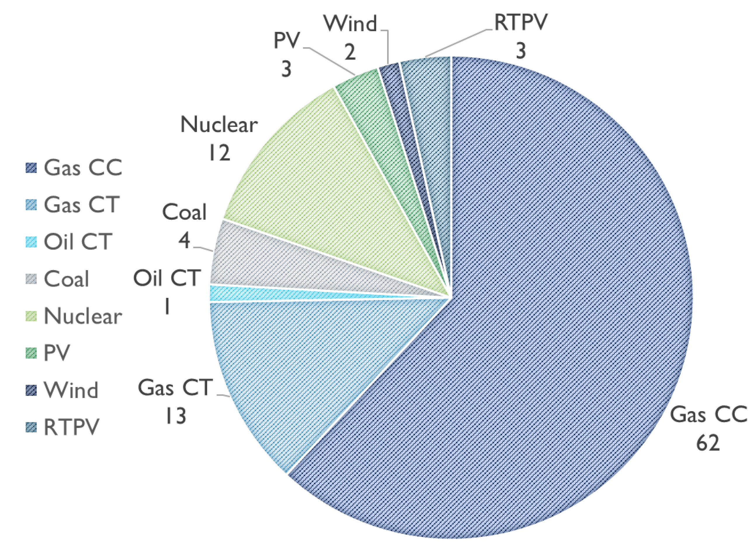
The NAU 5-bus system has an installed generation capacity that is representative of a utility in the southwestern U.S. (see
Figure 10). The researchers scaled the load from region 1 of the RTS-GMLC down to 1580 MW and applied it to the NAU 5-bus system. This peak load of 1580 MW matches the peak load in the “Pennsylvania-New Jersey-Maryland (PJM) 5-bus system”, from which the NAU 5-bus system drew its inspiration [
45]. Similarly, VRE sources were also scaled down from region 1 in the RTS-GMLC to the NAU 5-bus system. The capacity of the generators used in the NAU 5-bus system is shown in
Table 1. The time-series data for load and VRE are the actual real-time (RT) of a 1-h resolution in the RTS-GMLC.
Refer to
Table 2 for the load distribution per node in the NAU 5-bus system, which is similar to that of the PJM 5-bus system, except for the additional EV load in node C. A summary of the dispatchable generation fleet of the NAU 5-bus system is presented in
Table 3. The prices of various fuels are considered for the year 2025. The transmission parameters for the NAU 5-bus system are the same as those in the PJM 5-bus system [
45].
2.5. Production Cost Model
As mentioned, this research aimed to create models of EV load that are suitable for studying the integration of EVs into power system operations via a power system production cost model. Thus, the time resolution in the models is 1 h to replicate the day-ahead electricity market integration of EV charging. The objective of the PCM is to minimize the electricity generation cost, subject to a host of power system constraints. Production costs depend on a variety of factors, including the characteristics of the load and the generation on each node, the capabilities of the interconnecting transmission elements, the reserve requirements, the accuracy of load and VRE forecasts, etc. Consequently, the electricity prices at each node, i.e., the LMPs, often differ from one another. LMPs are an important output from a PCM and are typically higher during the peak load hours and lower during the off-peak hours. Due to the variation in the LMP with the time of day, a price-based charging strategy is a good choice for minimizing operating costs and reducing charging costs.
2.5.1. Power System Optimizer (PSO)
An appropriate PCM tool for this research requires capabilities similar to those typical in power system planning and operations. Polaris Systems Optimization’s power system optimizer (PSO) is a tool with the capabilities that are necessary for an accurate simulation of power system operations that mimics the actions and timing of power system planners and operators. PSO uses MILP, has multilevel nested time intervals (overlapping time frames), and simulates uncertainties for both load and VRE resource forecasting [
35]. Using multilevel nested time intervals means that the solver can commit units at multiple points in the time ahead of the hour of operation (e.g., commit units with long start-up time days ahead, units with 12-h start-up times a day ahead, units with a 1-h start-up time 1 h ahead, etc.). PSO also employs a “look-ahead” feature that permits commitment decisions to be made in full consideration of forecasted load and VRE beyond the current decision cycle. This multilevel nested time interval capability is important because it emulates the forecast uncertainties that system operators face in committing generators and ancillary services.
For this simulation, the planning cycle for committing units was a day ahead. It had a collection of horizons consisting of 24 1-h periods with a look-ahead of 24 h, and the time increment for dispatch (i.e., the period resolution) was hourly. The look-ahead ensures that the commitment decisions in every horizon are related to the expected conditions in the next horizon. The PCM outputs analyzed to show the effect of the EVs include total production cost (USD), generation (energy produced in megawatt hours; MWh), revenue (USD), and electricity price (LMP, USD/MWh). The revenue (USD) is calculated as the LMP (USD/MWh) times the generation (MWh). Therefore, the EV charging cost is equivalent to the negative of the revenue for the EV load. The model simulated seven days, using RTS-GMLC data from Wednesday 31 January to Tuesday 4 February. Net loads were low at times when the VRE was relatively high. The model run started on Wednesday and finished on Tuesday to ensure that the commitment on Sunday (the day for which analyzed the results) was in accordance with the previous and future power system conditions (i.e., there was sufficient time in advance of Sunday to start the slowest starting coal units). In the NAU 5-bus system on Sunday 2 February, the VRE reached its highest hourly penetration of 18% of the load between 11 a.m. and 1 p.m.
For each time increment of the model data, the “net load” that the conventional, dispatchable generation must serve is found by subtracting the VRE from the load on each bus. During system operation, dispatchable generators are committed and dispatched to serve the net load. The heat curves (heat rates) of the dispatchable generators listed in
Table 3 (taken from RTS-GMLC) are multiplied by their fuel costs to calculate the dispatch curves (cost curves), which have units of USD/MWh (refer to
Figure A1).
2.5.2. EV Penetration and Modeling
Regarding the quantity of EVs, we tested 1000 EVs. Given the assumed EV characteristics and their availability profile, this represented a maximum possible EV load of 2.8 MW during the morning hours, and about 0.8 MW during the midday hours (refer to
Figure 8). This was a small but realistic load penetration compared to the peak load of ~550 MW in the results to be presented in the next section. During periods of low load (e.g., night-time), fewer dispatchable generators will be online. Consequently, it is expected that any VRE or dispatchable load will be a more decisive factor influencing the system operation cost.
Within the PSO, the uncoordinated charging model was implemented as an “injector” with a discrete time series of EV load data points. These data resulted from the uncoordinated model previously described. To apply the coordinated charging model, we employed the built-in library “Energy Limited” (EL) in the PSO. The setup for this library requires an estimate of the amount of energy that needs to be served in a decision horizon (i.e., over the course of a day); this energy can be determined from the total daily energy supplied in the uncoordinated charging model, or by using the fleet’s daily energy consumption or total charging load in MWh. The dispatch constraint for the EVs is their charging availability, which represents the number of vehicles plugged into the grid; this number caps the power that can be drawn from the power network to charge the EVs in any time period (see
Figure 8). The EL library ensures that the total amount of the charging load is served, while honoring the EV availability constraints. For a detailed examination of the input data in PSO format (comma-separated values format), refer to the
Supplementary Materials.
3. Results
This section presents the results of running the PSO production cost model for the NAU 5-bus system for the week of interest. As a representative sample, the results of the simulation are presented for one day, in this case, 22 February, as it had the largest VRE penetration. This section starts by showing the results for the NAU 5-bus system with no EVs, followed by the results when charging 1000 EVs under the uncoordinated and coordinated charging scenarios.
3.1. System Operation without EVs
The generation stack and system LMPs for each hour of the day are presented in
Figure 11 for a typical day of operation in the period analyzed. The system LMP is represented by the dark dashed line and refers to the scale on the right side of the graph. The LMP varied between 24.6 USD/MWh at low net load, up to 35.4 USD/MWh during the peak load hours. The bars show the generation stack and refer to the scale on the left-hand side of the graph. The nuclear generation is represented by the green color on the bottom of each column and is the base load generation, which does not vary from hour to hour. The next generator stacked on each bar is the combined cycle (CC) gas generation (light blue color). This represents the marginal generator, and its output varies from hour to hour. Between hours 5 and 17, there was substantial VRE generation, represented by the small bars (dark blue, yellow, and red, respectively) stacked on the top of each bar. Note that the LMP increased and decreased as the CC generation changed, according to its cost curve (see
Figure A1 frame (e)). The LMP followed the expected behavior and had two peaks, one in the early morning and a higher second peak in the early evening. The LMP valley in the middle of the day was a consequence of high solar and wind power that reduced the net load. During this day, the total operation cost was calculated as 359,060 USD, the daily average system LMP was 29.65 USD, and the peak load was 551 MW at 18 h (6 p.m.).
3.2. System Operation with Uncoordinated EV Charging
Applying the uncoordinated charging model scaled to 1000 EVs resulted in the hourly EV load profile shown in
Figure 12. Uncoordinated EV charging had a maximum load of just under 1 MW at 20 h (8 p.m.), with a base load of just over 0.2 MW. The total energy consumed over the course of the day in charging the EVs was 10.75 MWh. The uncoordinated charging profile followed the trend of the EV arrivals (
Figure 5b), peaking in the early evening, as 85% of the charging happened at home.
Running the PCM PSO for the NAU 5-bus system with the addition of the EV load resulted in an operating cost of 359,390 USD (an increase of only 330 USD). In addition, the system LMP did not change; the system dispatch stack and LMP are similar to those shown in
Figure 11 because the EV charging profile was small compared with the rest of the injectors.
3.3. System Operation with Coordinated EV Charging
Implementing the coordinated charging modeling in the PSO resulted in the daily charging profile shown in
Figure 13. Recall that the coordinated charging model used the LMP in combination with EV availability and battery SoC in determining the time to charge as part of the goal to minimize operating costs over the course of a day. Compared with the uncoordinated charging profile (
Figure 12), most of the EV charging was moved to the low-LMP hours of the day (hours 1, 2, and 11 to 14). The total daily energy used in charging was the same as in the uncoordinated case (10.75 MWh), but the charging timing was shifted in a way that complied with EV charging availability, battery SoC, and daily charging requirement.
In the case of coordinated charging,
Figure 14 shows the generation stack and LMPs. The system operation cost for the day was 359,330 USD. Relative to the plot shown in
Figure 11, the system LMP increased between 1 a.m. and 2 a.m., which means that as the marginal generator increased its power dispatch due to the EV load, it increased a step in its cost curve.
Figure 15 directly compares this point, plotting the EV charging profiles and the system LMPs. Regardless of this increase in LMP, the overall production cost was less than for the case of uncoordinated charging, as the charging occurred during the lower-cost (i.e., lower LMP) hours during the day.
3.4. Comparing the EV Cost of Charging
The cost to charge the EVs was determined by multiplying the magnitude of energy used to charge the EVs each hour by the LMP that hour. The total cost to charge was then computed by summing the hourly charging costs over all hours of the day. The uncoordinated charging approach led to a cost to charge of 334 USD, while the coordinated charging cost was 294 USD (see
Figure 16). Using the coordinated charging approach reduced the cost of charging by 40 USD, equal to 12%. Interestingly, the system production cost decreased by 60 USD between the uncoordinated and coordinated cases, which was slightly different from the reduction in cost to a charge of 40 USD. This phenomenon is due to the coordinated EV charging profile changing the LMP in the early morning hours. Putting the charging numbers into a per vehicle context, the average EV will charge 10.75 kWh. The average uncoordinated charging cost was close to 0.33 USD per day per vehicle, and the coordinated charging cost was close to 0.29 USD, representing roughly 12% in savings. These numbers are representative of the low energy cost experienced by EV owners.
4. Discussion
Figure 17 shows a graph of the system and the EV loads for the day of 2 February, the same day as is presented in the previous figures with the dispatch stacks. The system load is shown by the light-blue bars (refers to the left-hand scale), and the EV load in the red (coordinated) and yellow (uncoordinated) bars, both referring to the right-hand scale and having a much lower magnitude than the system load. Compared to the system load alone, the uncoordinated EV charging increased the system’s peak load. In our particular simulation, 1000 EVs led to an increase in peak demand of 1 MW. Coordinated EV charging occurred during low-LMP hours and therefore did not increase the peak load.
It is interesting to compare operating costs and LMPs for each of the cases. In
Figure 18, the operation cost is shown in the blue columns associated with the primary
y axis on the left. In addition, in
Figure 18, the average LMP is shown by the orange line related to the secondary
y axis on the right. In this figure, the left column is for the system operation with no EV with a cost of 359,060 USD, the central column is for the system operation with uncoordinated EV charging with a cost of 359,390 USD, and the right column is for the system operation with coordinated EV charging with a cost of 359,330 USD. Thus, as shown by comparing the central and right columns with the left one, the addition of the EV load increased the system operation cost. However, the EV coordinated charging profile (right blue column) led to lower operating costs than the uncoordinated charging profile (central column). At the same time, the daily average LMP increased slightly (in 0.47 USD) with coordinated charging (right line). This is not uncommon in power system operation; average LMPs can increase while system operating costs decrease.
5. Conclusions
The purpose of this work was to create statistical models for EV charging that were suitable for power system operation. Statistical models for EV charging were created using data from the EV Project. This modeling with the appropriate data resulted in reasonable and scalable EV charging load profiles. The models recognized coordinated and uncoordinated charging loads. A production cost model could integrate the EV charging model and assess the EV effects on the power system cost and loads.
The modeling of uncoordinated and coordinated charging profiles required the battery size and charging level (power kW). In addition, the arrival time and planned energy consumption were necessary (i.e., the initial and final SoC). However, for coordinated charging, both the arrival and departure, or the equivalent availability, plus the energy or charging requirement (MWh) for the whole fleet were required.
Statistical modeling recreated the uncoordinated charging profile. A Monte Carlo simulation technique modeled the uncoordinated charging profile of each vehicle by sampling the initial SoC, final SoC, charging level, and arrival time as the start time of charging. The fleet charging profile was the sum of the individual charging profiles. The statistical analysis chi-square method was used to find the best fit distribution for the initial and final SoC. The best fit for the initial SoC was a beta distribution, and two beta distributions for the final SoC. The least-mean-square method provided the beta parameters to fit the data to beta distributions.
The authors developed an algorithm for modeling the uncoordinated charging and incorporated the result into the PCM model as a time series, similar to the load forecast or VRE forecast. However, coordinated charging modeling must be part of the PCM and modeled as a controllable load with the constraints imposed by the fleet characteristics, energy requirement (MWh), charging availability, and charging level (kW). Otherwise, the modeling will neglect the influence of the EV fleet on the electricity price.
The NAU 5-bus system, a simple 5-bus power system similar to the PJM 5-bus model but with time-series data from the RTS-GMLC model, was created to test the statistical models of the EVs. Polaris Systems Optimization’s PSO was the PCM used for this demonstration, and it showed the potential effects of 1000 EVs (maximum demand of ~0.2% of the NAU 5-bus peak load) on power system operating costs, LMPs, and dispatch stacks when implementing the two charging strategies mentioned above. The demonstration showed interesting results, and revealed the potential positive or negative effects of EVs on system operation. Coordinated charging exemplified the positive effects of accommodating EV charging coincident with VRE. However, uncoordinated charging demonstrated the negative effect of increasing the system peak load. With scalable statistical models of EVs, such as those presented here, it is possible to investigate the impact of charging strategies for the large-scale adoption of EVs on power system operations and costs.
Supplementary Materials
The following are available online at
https://www.mdpi.com/article/10.3390/wevj12040263/s1, File S1: PSO input files, File S2: System Operation with Coordinated EV Charging: EL EV_7days, File S3: System Operation without EVs: noev_7days, File S4: System Operation with Uncoordinated EV charging: UNCO_7days.
Author Contributions
Conceptualization, J.D.A.G., R.S., B.B. and T.L.A.; methodology, J.D.A.G., R.S., B.B. and T.L.A.; software, J.D.A.G., R.S. and B.B.; validation, J.D.A.G.; formal analysis, J.D.A.G., R.S. and B.B.; investigation, J.D.A.G., R.S. and B.B.; resources, T.L.A. and R.C.; data curation, J.D.A.G., R.S. and B.B.; writing—original draft preparation, J.D.A.G.; writing—review and editing, T.L.A. and R.C.; visualization, J.D.A.G.; supervision, T.L.A. and R.C.; project administration, J.D.A.G. All authors have read and agreed to the published version of the manuscript.
Funding
This research received no external funding.
Institutional Review Board Statement
Not applicable.
Informed Consent Statement
Not applicable.
Data Availability Statement
Acknowledgments
Polaris Systems Optimization for providing PSO and support, AIMMS for providing an academic license of AIMMS and CPLEX, and NREL for providing the RTS-GMLC model.
Conflicts of Interest
The authors declare no conflict of interest.
Appendix A. Cost Curves NAU 5-Bus System
Dispatch or cost curves of the committable generators presented in the NAU 5-bus system, showing the variable cost of producing a unit of energy with respect to the power output of these generators: (a) 121_NUCLEAR_1; (b) 101_STEAM_3 Coal; (c) 113_CT_1, 2, 3, 4 NG; (d) 102_CT_1 Oil; (e) 118_CC_1; (f) 117_CC_1; (g) 213_CC_3.
Figure A1.
Dispatch or cost curves of the committable generators presented in the NAU 5-bus system, showing the variable cost of producing a unit of energy with respect to the power output these generators: (a) nuclear steam unit: 121_NUCLEAR_1; (b) coal steam unit: 101_STEAM_3 Coal; (c) natural gas (NG) combustion turbine (CT): 113_CT_1, 2, 3, 4 NG; (d) oil-fueled CT: 102_CT_1 Oil; (e) natural gas combined cycle (CC):118_CC_1; (f) 117_CC_1; (g) 213_CC_3.
References
- McKerracher, C. Electric Vehicle Outlook 2017. Blomberg Finance L.P. 2017. Available online: https://data.bloomberglp.com/bnef/sites/14/2017/07/BNEF_EVO_2017_ExecutiveSummary.pdf (accessed on 19 August 2019).
- Enerdata. Up to 50% of the Global Car Fleet Could Be Electric* in 2050 Executive Brief. 2018. Available online: https://www.enerdata.net/publications/executive-briefing/half-vehicles-cars-will-be-electrical-2050.pdf (accessed on 19 August 2019).
- Chediak, M. The Latest Bull Case for Electric Cars: The Cheapest Batteries Ever—Bloomberg. 2017. Available online: https://www.bloomberg.com/news/articles/2017-12-05/latest-bull-case-for-electric-cars-the-cheapest-batteries-ever (accessed on 14 September 2018).
- Henze, V. Battery Pack Prices Cited Below $100/kWh for the First Time in 2020, While Market Average Sits at $137/kWh; BloombergNEF Press: New York, NY, USA, 2020; Available online: https://about.bnef.com/blog/battery-pack-prices-cited-below-100-kwh-for-the-first-time-in-2020-while-market-average-sits-at-137-kwh/ (accessed on 18 April 2021).
- Fulton, L.M.; Seleem, A.; Boshell, F.; Salgado, A.; Saygin, D. Electric Vehicles Technology Brief; IRENA: Abu Dhabi, United Arab Emirates, 2017; Available online: http://www.irena.org/-/media/Files/IRENA/Agency/Publication/2017/IRENA_Electric_Vehicles_2017.pdf (accessed on 19 August 2019).
- Wood, E.; Rames, C.; Muratori, M.; Raghavan, S.; Melaina, M. National Plug-In Electric Vehicle Infrastructure Analysis. 2017. Available online: https://www.energy.gov/sites/default/files/2017/09/f36/NationalPlugInElectricVehicleInfrastructureAnalysis_Sept2017.pdf (accessed on 19 August 2019).
- Muratori, M.; Moran, M.J.; Serra, E.; Rizzoni, G. Highly-resolved modeling of personal transportation energy consumption in the United States. Energy 2013, 58, 168–177. [Google Scholar] [CrossRef]
- Muratori, M. Impact of uncoordinated plug-in electric vehicle charging on residential power demand. Nat. Energy 2018, 3, 193–201. [Google Scholar] [CrossRef]
- Kintner-Meyer, M.; Schneider, K.; Pratt, R. Impacts Assessment of Plug-In Hybrid Vehicles on Electric Utilities and Regional U.S. Power Grids; PNNL: Richland, WA, USA, 2007. Available online: https://energyenvironment.pnnl.gov/ei/pdf/PHEV_Feasibility_Analysis_Part1.pdf (accessed on 18 July 2018).
- Luo, Z.; Hu, Z.; Song, Y.; Xu, Z.; Lu, H. Optimal coordination of plug-in electric vehicles in power grids with cost-benefit analysis—Part I: Enabling techniques. IEEE Trans. Power Syst. 2013, 28, 3546–3555. [Google Scholar] [CrossRef]
- Tuffner, F.; Kintner-Meyer, M. Using Electric Vehicles to Meet Balancing Requirements Associated with Wind Power; PNNL: Richland, WA, USA, 2011.
- Schey, S.; Scoffield, D.; Smart, J. A First Look at the Impact of Electric Vehicle Charging on the Electric Grid in The EV Project. World Electr. Veh. J. 2012, 5, 667–668. [Google Scholar] [CrossRef] [Green Version]
- Sokorai, P.; Fleischhacker, A.; Lettner, G.; Auer, H. Stochastic modeling of the charging behavior of electromobility. World Electr. Veh. J. 2018, 9, 44. [Google Scholar] [CrossRef] [Green Version]
- Wang, Y.; Infield, D. Markov Chain Monte Carlo simulation of electric vehicle use for network integration studies. Int. J. Electr. Power Energy Syst. 2018, 99, 85–94. [Google Scholar] [CrossRef]
- Ul-Haq, A.; Azhar, M.; Mahmoud, Y.; Perwaiz, A.; Al-Ammar, E.A. Probabilistic modeling of electric vehicle charging pattern associated with residential load for voltage unbalance assessment. Energies 2017, 10, 1351. [Google Scholar] [CrossRef]
- Grahn, P. Electric Vehicle Charging Modeling. Ph.D. Thesis, KTH Royal Institute of Technology, Stockholm, Sweden, October 2013. Available online: http://news.hydroquebec.com/media/filer_private/2013/11/28/fiche_dinformation_recharge_vfinaleang.pdf (accessed on 4 August 2018).
- Chung, Y.-W.; Khaki, B.; Li, T.; Chu, C.; Gadh, R. Ensemble machine learning-based algorithm for electric vehicle user behavior prediction. Appl. Energy 2019, 254, 113732. [Google Scholar] [CrossRef]
- Lahariya, M.; Benoit, D.F.; Develder, C. Synthetic Data Generator for Electric Vehicle Charging Sessions: Modeling and Evaluation Using Real-World Data. Energies 2020, 13, 4211. [Google Scholar] [CrossRef]
- Lin, H.; Liu, Y.; Sun, Q.; Xiong, R.; Li, H.; Wennersten, R. The impact of electric vehicle penetration and charging patterns on the management of energy hub—A multi-agent system simulation. Appl. Energy 2018, 230, 189–206. [Google Scholar] [CrossRef]
- Olivella-Rosell, P.; Villafafila-Robles, R.; Sumper, A.; Bergas-Jané, J. Probabilistic agent-based model of electric vehicle charging demand to analyse the impact on distribution networks. Energies 2015, 8, 4160–4187. [Google Scholar] [CrossRef]
- Sheppard, C.; Waraich, R.; Gopal, A.R.; Campbell, A.; Pozdnukov, A. Modeling Plug-in Electric Vehicle Charging Demand with BEAM, the Framework for Behavior Energy Autonomy Mobility; LBNL: Berkeley, CA, USA, 2017. Available online: https://eta-publications.lbl.gov/sites/default/files/lbnl-2001018.pdf (accessed on 7 February 2019).
- Lin, H.; Fu, K.; Liu, Y.; Sun, Q.; Wennersten, R. Modeling charging demand of electric vehicles in multi-locations using agent-based method. Energy Procedia 2018, 152, 599–605. [Google Scholar] [CrossRef]
- Lopez, N.S.; Allana, A.; Biona, J.B.M. Modeling Electric Vehicle Charging Demand with the Effect of Increasing EVSEs: A Discrete Event Simulation-Based Model. Energies 2021, 14, 3734. [Google Scholar] [CrossRef]
- Værbak, M.; Ma, Z.; Demazeau, Y.; Jørgensen, B.N. A generic agent-based framework for modeling business ecosystems: A case study of electric vehicle home charging. Energy Inform. 2021, 4, 28. [Google Scholar] [CrossRef]
- Nguyen, K.; Schumann, R. A socio-psychological modal choice approach to modelling mobility and energy demand for electric vehicles. Energy Inform. 2020, 3, 20. [Google Scholar] [CrossRef]
- Lee, R.; Yazbeck, S.; Brown, S. Validation and application of agent-based electric vehicle charging model. Energy Rep. 2020, 6, 53–62. [Google Scholar] [CrossRef]
- Heinisch, V.; Göransson, L.; Erlandsson, R.; Hodel, H.; Johnsson, F.; Odenberger, M. Smart electric vehicle charging strategies for sectoral coupling in a city energy system. Appl. Energy 2021, 288, 116640. [Google Scholar] [CrossRef]
- Stiasny, J.; Zufferey, T.; Pareschi, G.; Toffanin, D.; Hug, G.; Boulouchos, K. Sensitivity analysis of electric vehicle impact on low-voltage distribution grids. Electr. Power Syst. Res. 2021, 191, 106696. [Google Scholar] [CrossRef]
- Moon, J.H.; Gwon, H.N.; Jo, G.R.; Choi, W.Y.; Kook, K.S. Stochastic Modeling Method of Plug-in Electric Vehicle Charging Demand for Korean Transmission System Planning. Energies 2020, 13, 4404. [Google Scholar] [CrossRef]
- Jadun, P.; McMillan, C.; Steinberg, D.; Muratori, M.; Vimmerstedt, L.; Mai, T. Electrification Futures Study: End-Use Electric Technology Cost and Performance Projections through 2050; NREL: Golden, CO, USA, 2017. Available online: https://www.nrel.gov/docs/fy18osti/70485.pdf (accessed on 18 July 2018).
- Davis, M. Total Cost of Ownership for Current Plug-In Electric Vehicles, Update to Model 2013 and 2014 Model Year Vehicles; Rep. 3002004054; EPRI: Palo Alto, CA, USA, 2014; Available online: https://www.epri.com/research/products/000000003002004054 (accessed on 18 July 2018).
- U.S. Department of Energy Alternative Fuels Data Center: Vehicle Cost Calculator. Available online: https://afdc.energy.gov/calc/ (accessed on 12 July 2021).
- Rissman, J. The Future of Electric Vehicles in the U.S.; Energy Innov. Policy & Technol. LLC: San Francisco, CA, USA, 2017; Available online: http://energyinnovation.org/wp-content/uploads/2017/09/2017-09-13 (accessed on 23 July 2018).
- Guy, J.D. Security Constrained Unit Commitment. IEEE Trans. Power Appar. Syst. 1971, PAS-90, 1385–1390. [Google Scholar] [CrossRef]
- Polaris Systems Optimization Power System Optimizer (PSO). Available online: http://psopt.com/pso/ (accessed on 10 September 2018).
- Shrestha, R. Uncoordinated and Price Incentive Based Load Profiles Due to Electric Vehicle Charging. Master’s Thesis, Northern Arizona University, Flagstaff, AZ, USA, 2019. Available online: https://www.proquest.com/docview/2369458122/fulltextPDF/48EE3FB51EE44BCEPQ/1?accountid=12706 (accessed on 5 September 2021).
- Bhattarai, B. Aggregator Based Charging Management of Electric Vehicles. Master’s Thesis, Northern Arizona University, Flagstaff, AZ, USA, 2019. Available online: https://www.proquest.com/docview/2377906639?pq-origsite=primo (accessed on 5 September 2021).
- Dunckley, J. Electric Vehicle Driving, Charging, and Load Shape Analysis: A Deep Dive into Where, When, and How Much Salt River Project (SRP) Electric Vehicle Customers Charge; Rep. 3002013754; EPRI: Palo Alto, CA, USA, 2018; Available online: https://www.epri.com/research/products/000000003002013754 (accessed on 27 July 2020).
- Weisstein, E.W. Beta Distribution; MathWorld, Wolfram Web Resource. Available online: https://mathworld.wolfram.com/BetaDistribution.html (accessed on 20 November 2019).
- Smart, J.; Schey, S. Battery Electric Vehicle Driving and Charging Behavior Observed Early in The EV Project. SAE Int. J. Altern. Powertrains 2012, 1, 27–33. [Google Scholar] [CrossRef] [Green Version]
- INL. EV Project Electric Vehicle Charging Infrastructure Summary Report Period: January–December 2013; INL/MIS-10-19479; Idaho Natl. Labratory: Idoha Falls, ID, USA, October 2014. Available online: https://avt.inl.gov/sites/default/files/pdf/EVProj/EVProjectInfrastructureReportJan13Dec13.pdf (accessed on 13 January 2020).
- Vujic, J.L. Monte Carlo Sampling Methods; Nuclear Engineering Department University of California: Berkeley, CA, USA, 2004; Available online: http://web.tecnico.ulisboa.pt/~mcasquilho/acad/theo/simul/Vujic.pdf (accessed on 13 January 2020).
- Barrows, C. Reliability Test System of the Grid Modernization Laboratory Consortium (RTS-GMLC); NREL: Golden, CO, USA, 2018. Available online: https://github.com/GridMod/RTS-GMLC/blob/master/RTS-GMLC.pdf. (accessed on 18 July 2018).
- Barrows, C.; Bloom, A.; Ehlen, A.; Ikäheimo, J.; Jorgenson, J.; Krishnamurthy, D.; Lau, J.; McBennett, B.; O’Connell, M.; Preston, E.; et al. The IEEE Reliability Test System: A Proposed 2019 Update. IEEE Trans. Power Syst. 2020, 35, 119–127. [Google Scholar] [CrossRef]
- Li, F.; Bo, R. Small test systems for power system economic studies. In Proceedings of the IEEE PES General Meeting, Minneapolis, MN, USA, 25–29 July 2010; pp. 1–4. [Google Scholar] [CrossRef]
Figure 1.
Charging level proportion (%) modeled in the electric vehicle (EV) fleet.
Figure 1.
Charging level proportion (%) modeled in the electric vehicle (EV) fleet.
Figure 2.
A plot of the beta distribution model of the initial state-of-charge (SoC) values fitted to the source data.
Figure 2.
A plot of the beta distribution model of the initial state-of-charge (SoC) values fitted to the source data.
Figure 3.
Beta distributions fitted to the target state-of-charge source data.
Figure 3.
Beta distributions fitted to the target state-of-charge source data.
Figure 4.
Weekday charging availability covering all types of chargers in the EV Project 2013 [
41].
Figure 4.
Weekday charging availability covering all types of chargers in the EV Project 2013 [
41].
Figure 5.
EV availability in the EV Project data during weekdays as (
a) departures and (
b) arrivals [
41].
Figure 5.
EV availability in the EV Project data during weekdays as (
a) departures and (
b) arrivals [
41].
Figure 6.
Flowchart of EV uncoordinated load modeling.
Figure 6.
Flowchart of EV uncoordinated load modeling.
Figure 7.
Flowchart of the modeled aggregator.
Figure 7.
Flowchart of the modeled aggregator.
Figure 8.
Projected maximum power (P) in MW for 1000 EVs on a weekday based on charging availability and charging capacity.
Figure 8.
Projected maximum power (P) in MW for 1000 EVs on a weekday based on charging availability and charging capacity.
Figure 9.
Northern Arizona University (NAU) 5-bus system layout that portrays buses (bold vertical lines), transmission lines (connecting the buses), loads (inverted triangles), and generators (circles and rectangles).
Figure 9.
Northern Arizona University (NAU) 5-bus system layout that portrays buses (bold vertical lines), transmission lines (connecting the buses), loads (inverted triangles), and generators (circles and rectangles).
Figure 10.
Proportion ratio (%) for the types of generators considered in the NAU 5-bus system (CC = combined cycle; CT = combustion turbine; PV = photovoltaics; RTPV = rooftop PV).
Figure 10.
Proportion ratio (%) for the types of generators considered in the NAU 5-bus system (CC = combined cycle; CT = combustion turbine; PV = photovoltaics; RTPV = rooftop PV).
Figure 11.
Power generation (Pg) stack MW (left axis) and locational marginal price (LMP) USD/MWh (right axis) in the NAU 5-bus system occurring without EVs.
Figure 11.
Power generation (Pg) stack MW (left axis) and locational marginal price (LMP) USD/MWh (right axis) in the NAU 5-bus system occurring without EVs.
Figure 12.
Uncoordinated EV charging power (P) profile in MW developed for 1000 EVs.
Figure 12.
Uncoordinated EV charging power (P) profile in MW developed for 1000 EVs.
Figure 13.
Coordinated EV charging power (P) profile in MW developed for 1000 EVs.
Figure 13.
Coordinated EV charging power (P) profile in MW developed for 1000 EVs.
Figure 14.
Power generation (Pg) stack MW (left axis) and LMP USD/MWh (right axis) in the NAU 5-bus system occurring with coordinated EV charging.
Figure 14.
Power generation (Pg) stack MW (left axis) and LMP USD/MWh (right axis) in the NAU 5-bus system occurring with coordinated EV charging.
Figure 15.
Comparison of the EV coordinated and EV uncoordinated charging profile power (P) in MW (left axis) and their corresponding system LMPs in USD/MWh (right axis).
Figure 15.
Comparison of the EV coordinated and EV uncoordinated charging profile power (P) in MW (left axis) and their corresponding system LMPs in USD/MWh (right axis).
Figure 16.
Comparison between the coordinated and uncoordinated cost in USD of EV charging for 1000 EVs.
Figure 16.
Comparison between the coordinated and uncoordinated cost in USD of EV charging for 1000 EVs.
Figure 17.
Comparison of the system load (L) in MW (left axis) against the EV coordinated and EV uncoordinated charging power (P) profiles (right axis) of 1000 EVs.
Figure 17.
Comparison of the system load (L) in MW (left axis) against the EV coordinated and EV uncoordinated charging power (P) profiles (right axis) of 1000 EVs.
Figure 18.
Summary of the system operation cost and LMP change with the introduction of EV charging, gross comparison against the system with no EVs.
Figure 18.
Summary of the system operation cost and LMP change with the introduction of EV charging, gross comparison against the system with no EVs.
Table 1.
Generation capacity per technology and penetration percentage presented in the NAU 5-bus system.
Table 1.
Generation capacity per technology and penetration percentage presented in the NAU 5-bus system.
| Generation Technology | Capacity (MW) | Percentage (%) |
|---|
| Gas CC | 1065 | 62 |
| Gas CT | 220 | 13 |
| Oil CT | 20 | 1 |
| Coal | 76 | 4 |
| Nuclear | 200 | 12 |
| PV | 54 | 3 |
| Wind | 28 | 2 |
| RTPV | 59 | 3 |
| TOTAL | 1722 | 100 |
Table 2.
Load distribution presented in the NAU 5-bus system.
Table 2.
Load distribution presented in the NAU 5-bus system.
| Node | System Load (%) | EV Load (%) |
|---|
| A | 0% | 0% |
| B | 30% | 0% |
| C | 30% | 100% |
| D | 40% | 0% |
| E | 0% | 0% |
Table 3.
Summary of dispatchable generators in the NAU 5-bus system.
Table 3.
Summary of dispatchable generators in the NAU 5-bus system.
| Node | Name | Type | Fuel | Fuel Price 1 (USD/MMBtu) | Max Dispatch (MW) | Min Dispatch (MW) | Cold Start (USD/MWh) |
|---|
| E | 107_CC_1 | Combined Cycle | Natural Gas | 4.2 | 355 | 170 | 30,303 |
| E | 118_CC_1 |
| C | 213_CC_1 |
| D | 102_CT_1 | Combustion Turbine | Oil | 23.9 | 20 | 8 | 120 |
| A | 101_STEAM_3 | Steam Turbine | Coal | 2.8 | 76 | 30 | 8600 |
| A | 121_NUCLEAR_1 | Steam Turbine | Nuclear | 0.8 | 200 | 198 | 31,600 |
| D | 113_CT_1 | Combustion Turbine | Natural Gas | 4.2 | 55 | 22 | 6121 |
| D | 113_CT_2 |
| C | 113_CT_3 |
| C | 113_CT_4 |
| Publisher’s Note: MDPI stays neutral with regard to jurisdictional claims in published maps and institutional affiliations. |
© 2021 by the authors. Licensee MDPI, Basel, Switzerland. This article is an open access article distributed under the terms and conditions of the Creative Commons Attribution (CC BY) license (https://creativecommons.org/licenses/by/4.0/).


 ,
, 


