MPC-Based Obstacle Avoidance Path Tracking Control for Distributed Drive Electric Vehicles

Abstract

A path tracking controller based on front wheel steering angle and additional yaw moment control is designed to achieve safe obstacle avoidance of distributed drive electric vehicles. Using sixth-degree polynomial at a given time with anti-collision and anti-rollover conditions, the path planning of obstacle avoidance is proposed. The front wheel steering angle and additional yaw moment are output by the Model Predictive Control (MPC) controller. The wheel torque is distributed by the torque distribution controller. Through additional yaw moment and the vertical force ratio of the wheel, the obstacle avoidance path tracking control is realized. The co-simulation platform is established with Carsim/Simulink. The obstacle avoidance path, model predictive controller and torque distribution controller designed in this paper are simulated. The results show that obstacle avoidance path and tracking controller for the distributed drive electric vehicles effectively meet the requirements of safe obstacle avoidance.

1. Introduction

With the continuous increase in car ownership, the modern intelligent transportation system has increasingly regarded vehicle safety as its key factor. Between 2002 and 2012, the lack of proper obstacle avoidance contributed to the deaths of millions of people in traffic accidents around the world, and the economic cost of these accidents amounted to $0.48 trillion [1]. More than 90% of these accidents are caused by human factors [2]. Therefore, in order to avoid vehicle collisions and minimize the impact of accidents, a method of adding an increasing proportion of active safety systems is proposed [3].

The obstacle avoidance trajectory tracking control of intelligent vehicles is one of the key functions. According to the trajectory planned by the upper controller and the real-time state information, real-time vehicle control variables, such as front wheel angle and driving force/braking force, are generated [4]. Compared with traditional vehicles, the drive motors are directly installed in the drive wheels for the distributed drive electric vehicles. So they have outstanding advantages, such as short drive transmission chain, high transmission efficiency and compact structure. It can be more beneficial to realize the tracking control of the obstacle avoidance path by optimizing the distribution of the driving torque of each wheel [5]. Although distributed hub motors can lead to greater unsprung mass, a small amount of unsprung mass increase is negligible, given their advantages in dynamic control.

After the continuous development of path tracking control, different tracking control algorithms have been proposed and verified, such as sliding mode control, fuzzy control, and model predictive control. Reference [6] proposed a distributed drive unmanned vehicle path tracking and stability coordinated control strategy based on the layered control theory. In order to reduce the heading deviation and lateral deviation during the path-tracking process, the sliding mode control method was used. Moreover, it can ensure the stability of the vehicle. On the basis of the traditional dynamic model and preview model, Zhang Bingli [7] designed a new trajectory-tracking controller based on neural networks and fuzzy control theory. Wang Yao [8] proposed a model prediction-fuzzy (MPC-Fuzzy) joint control strategy, which alleviated the conflict between the vehicle tracking accuracy and the controller’s computational pressure under a single model prediction control and better solved the distributed driving vehicle path, tracking accuracy and stability issues in tracking. Hu [9] designed a fuzzy linear quadratic regulator (LQR) with preview PID angle compensation and verified that it can maintain good accuracy and stability at different vehicle speeds. However, it also had the problem of low tracking accuracy when the vehicle was running at a low speed. Kou [10] used a state expansion MPC and corner compensation fuzzy controller, designed a dual feedback MPC controller based on state expansion and verified that it had better path tracking performance at medium and low vehicle speeds. Wu [11] proposed a front-wheel steering controller and optimized the controller parameters so that the vehicle had better path-tracking performance at low and medium speeds and ensured that the vehicle had certain steering accuracy and driving stability when driving at high speed on ice and snow roads. In order to improve the stability of distributed drive electric vehicles in extreme working conditions, Li [12] proposed a nonlinear model predictive control (NMPC) based torque coordination control strategy. In order to coordinate the trajectory tracking accuracy and stability of distributed drive electric vehicles and improve the adaptive ability of the control algorithm to different working conditions, Zhuang [13] proposed a trajectory tracking control strategy based on Takagi–Sugeno fuzzy model predictive control (T-S FMPC).

The total required torque is calculated through the yaw moment obtained by the upper controller. The torque distributed to each drive wheel is obtained through different algorithms. There are many distribution methods for torque distribution. A fixed proportional distribution method was proposed in the literature [14,15]. Although this method was simple, it cannot implement different proportional distributions according to different road conditions. There was no optimization in the energy utilization efficiency of the motor, and the best distribution result could not be achieved. Ono E [16] proposed to realize the torque distribution to the four wheels according to the usage of the tire force of four tires. This method made the wear degree of the four tires more balanced, and the life of the tires and the motor were improved, but the performance of vehicle handling was greatly reduced. Mokhiamar O [17] also proposed to analyze the torque distribution problem by establishing a multi-objective optimization function, but this method may show different effects in different models and different operating conditions, so the consistency and robustness were poor. Reference [18] considered the dynamic characteristics of the vehicle when it is unstable and proposed a control allocation scheme based on feedback linearization. This scheme was relatively dependent on the accuracy of the model and had poor stability. Reference [19] distributed torque according to the vertical load distribution ratio of each wheel. Since the friction ellipse of the tire increases with the increase of the vertical load, the torque distribution according to the vertical load ratio of a single tire can avoid the saturation of the tire force and can simply and effectively improve the driving stability of the vehicle.

Based on the above analysis, the whole vehicle control process designed in this paper is shown in Figure 1. In Section 1, using the obstacle information obtained by the environment awareness layer and the vehicle pose information detected by the vehicle sensor, the obstacle avoidance path is planned. Anti-collision and anti-rollover constraints adding to a six-degree polynomial are used for path planning. The front wheel angle δ_f and additional yaw moment ∆M_z are output by the MPC controller in Section 3.2. By processing the information of the path planning layer, the torque distribution controller distributes the torque through the additional yaw moment and the wheel vertical force ratio in Section 3.3. The MPC controller and the torque distribution controller together form a path-tracking controller. During the obstacle avoidance process, the vehicle avoids obstacles through the front wheel angle and four-wheel torque output by the controller. In Section 4, the simulation platform is established, and the effect of the controllers is verified.

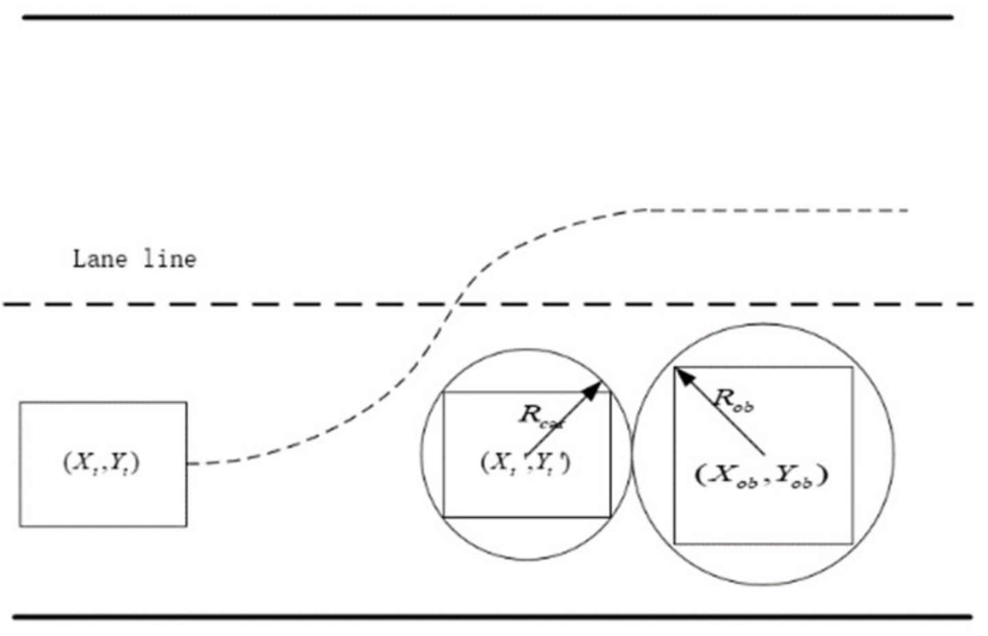
2. Path Planning

In this paper, the six-degree polynomial path planning method [20] for a given time is used. In the sixth-degree polynomial path planning method, the vehicle’s gentle arrival from the starting point to the target point is considered, the collision between the vehicle and the obstacle in the process of running is considered, and the smooth running according to the planned path is also considered. With the addition of anti-collision and anti-rollover conditions, the safety of obstacle avoidance path planning is improved.

Based on the longitudinal and lateral displacements at a given time, the initial expression for the sixth-degree polynomial is:

$$\{\begin{array}{l}X\left(t\right)={\mathrm{c}}_0+c_{1}t+c_2{t}^2+c_3{t}^3+c_4{t}^4+c_5{t}^5+c_6{t}^6\\ Y\left(t\right)=b_0+b_{1}t+b_2{t}^2+b_3{t}^3+b_4{t}^4+b_5{t}^5+b_6{t}^6\end{array}$$

(1)

Adding anti-collision conditions [20]: set the coordinate center of the obstacle as (X_ob, Y_ob), and the radius of the circumscribed circle of the vehicle and the obstacle as R_car and R_ob, this is shown in Figure 2,the constraint condition of anti-collision can be expressed as:

$${(R_{car}+R_{ob})}^2<{[X\left(t\right)-X_{ob}]}^2+{[Y\left(t\right)-Y_{ob}]}^2$$

(2)

Adding the anti-rollover condition constraint [20].

According to the simplified model diagram of vehicle rollover in Figure 3, the moment balance equation can be expressed as:

$$m_s{a}_{y}h+m_{s}g\Delta y=\left(F_{zl}-F_{zr}\right)\frac{s}{2}$$

(3)

where, a_y is the lateral acceleration, $m_s$ is the sprung mass, $h$ is the distance from the center of mass to the ground, $F_{zl}$ represents the sum of forces on the left front and rear wheels in the vertical direction, $F_{zr}$ represents the sum of forces on the right front and rear wheels, $s$ represents the track width, g is the gravitational acceleration, $\Delta y=h\cdot \sin \varphi$.

The lateral transfer rate of the vehicle is:

$$\mathrm{LTR}=\frac{F_{\mathrm{zl}}-F_{\mathrm{zr}}}{F_{\mathrm{zl}}+F_{\mathrm{zr}}}$$

(4)

Combining Equations (3) and (4), LTR can be expressed as:

$$LTR=\frac{2R}{s}\left[\frac{a_y}{g}+\sin \varphi \right]$$

(5)

where, ϕ is the vehicle roll angle.

The larger the absolute value of LTR indicates, the greater the rollover risk of the car, so the size of a_y should be fully taken into account in path planning. Given the maximum roll risk LTR_max,

$$a_y=\ddot{Y}\left(t\right)\le \left(\frac{s\cdot {\mathrm{LTR}}_{\max }}{2h}-\sin \varphi \right)g$$

(6)

$$a_{y\max }=\left(\frac{s\cdot {\mathrm{LTR}}_{\max }}{2h}-\sin \varphi \right)g$$

(7)

Constructing the evaluation index function of anti-rollover:

$$J_{anti-r}={\displaystyle {\int }_{t_0}^{{\mathrm{t}}_d}-\left(a_{y\max }-\left|a_y\right|\right)dt}$$

(8)

The polynomial optimization path planning problem is expressed as:

$$\{\begin{array}{l}\min J_{anti-r}\\ \mathrm{s}.\mathrm{t}.{\left(R_{car}+R_{ob}\right)}^2<{\left[X\left(t\right)-X_{ob}\right]}^2+{\left[Y\left(t\right)-Y_{ob}\right]}^2\\ a_y=\ddot{Y}\left(t\right)\le \left(\frac{s\cdot {\mathrm{LTR}}_{\max }}{2h}-\sin \varphi \right)g\\ b_3{t}_d{}^3+b_4{t}_d{}^4+b_5{t}_d{}^5+b_6{t}_d{}^6=H\\ 3b_3{t}_d{}^2+4b_4{t}_d{}^3+5b_5{t}_d{}^4+6b_6{t}_d{}^5=0\\ 6b_3{t}_d+12b_4{t}_d{}^2+20b_5{t}_d{}^3+30b_6{t}_d{}^4=0\end{array}$$

(9)

where, t₀ and t_d are the initial time and the end time, respectively, a_y is the lateral acceleration, X_ob and Y_ob are the coordinate centers of the obstacles, the coordinate center of the obstacle:(X_ob, Y_ob) = (100, 1), R_car and R_ob are the radiuses of the circumscribed circles between the vehicle and the obstacle, ∅ is the body roll angle, and w is the wheelbase, h is the distance from the center of mass to the ground, g is the acceleration of gravity, H is the self-conjugate matrix, J_anti-r is the anti-rollover evaluation index function, and LTR is the roll risk coefficient.

In Equation (9), the coefficients b₃, b₄, b₅ and b₆ can be obtained by the optimization algorithm.

The yaw angle can be expressed as:

$$\phi \left(t\right)=\arctan \frac{\mathrm{d}Y\left(t\right)}{\mathrm{d}X\left(t\right)}=\arctan \frac{\dot{Y}\left(t\right)}{\dot{X}\left(t\right)}$$

(10)

3. Path Tracking Control

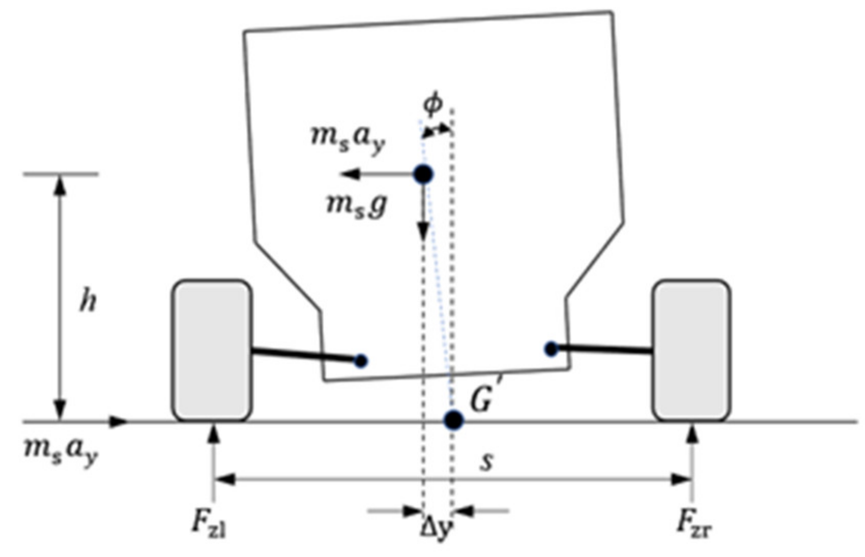
3.1. Establishment of Vehicle Dynamics Model

The three-degree-of-freedom vehicle dynamics model is shown in Figure 4, including lateral motion, yaw motion and longitudinal motion [21,22]. The aerodynamics, suspension system and steering system are ignored. Considering that the sideslip angle of the center of mass is small when the lateral acceleration is not high, the control accuracy will not be affected if it is ignored, so the sideslip angle of the center of mass is ignored [23]. According to the characteristics of the distributed drive vehicle, the additional yaw moment is considered.

In Figure 4, the coordinate axis oxyz is the fixed coordinate system of the vehicle, xoz is in the left-right symmetrical plane of the vehicle, the coordinate origin of the center of mass of the vehicle is o, the x-axis is the coordinate axis along the longitudinal direction of the vehicle, and the y-axis is the coordinate perpendicular to the longitudinal direction of the vehicle axis. The z-axis is the coordinate axis perpendicular to the xoy plane, and the direction satisfies the right-hand rule. XOY is the geodetic coordinate system. Considering that F_xf and F_yf are the force exerted on a single tire, it needs to be multiplied by 2. According to Newton’s second law:

$$\{\begin{array}{l}m\ddot{x}=m\dot{y}\dot{\phi }+2F_{xf}+2F_{xr}\\ m\ddot{y}=-m\dot{x}\dot{\phi }+2F_{yf}+2F_{yr}\\ I_z\ddot{\phi }=2l_f{F}_{yf}-2l_r{F}_{yr}\end{array}$$

(11)

where l_f and l_r are the distances from the center of mass to the front and rear axles, respectively. m is the overall mass of the vehicle, and I_z is the central moment of inertia of the vehicle around the z axis.

The conversion relationship between the resultant force of the tire in the x-direction and y-direction, the longitudinal force and the lateral force is expressed as follows:

$$\{\begin{array}{l}{F}_{xf}=F_{lf}\cos {\delta }_f-F_{cf}\sin {\delta }_f\\ F_{xr}=F_{lr}\cos {\delta }_f+F_{cr}\sin {\delta }_r\\ F_{yf}=F_{lf}\sin {\delta }_f+F_{cf}\cos {\delta }_f\\ F_{yr}=F_{cr}\cos {\delta }_r-F_{lr}\sin {\delta }_f\end{array}$$

(12)

where F_xf and F_yf are the resultant forces on the front wheels in the x and y directions, respectively. F_xr and F_yr are the resultant forces on the front wheels in the x and y directions, respectively, and F_lf and F_lr are the longitudinal forces on the front and rear wheels, respectively. F_cf and F_cr are the lateral forces on the front and rear wheels, respectively. δ_f is the front wheel angle, δ_r is the rear wheel angle.

The lateral and longitudinal forces of vehicle tires can be expressed as complex functions of parameters such as wheel slip angle, slip rate, road friction coefficient and vertical load:

$$F_c=f_c\left(\alpha ,s,\mu ,F_z\right)$$

(13)

$$F_l=f_l\left(\alpha ,s,\mu ,F_z\right)$$

(14)

where, F_z is the vertical load on the tire, μ is the road friction coefficient, s is the slip ratio, and α is the wheel side angle.

In order to simplify the model, the tire force is usually represented by a linear function under the condition of small tire longitudinal slip rate, lateral acceleration and slip angle. The force is expressed as follows:

$$\{\begin{array}{l}{F}_l=C_{l}s\\ F_c=C_c\alpha \end{array}$$

(15)

where C_l is the longitudinal stiffness of the vehicle tire, and C_c is the cornering stiffness of the vehicle tire.

The following approximate relationship is satisfied:

$$\{\begin{array}{l}\cos \theta \approx 1\\ \sin \theta \approx \theta \\ \tan \theta \approx \theta \end{array}$$

(16)

where θ can be expressed as front wheel side angle and rear wheel side slip angle, etc.

The wheel side slip angle α can be obtained according to the geometric relationship:

$$\alpha ={\tan }^{-1}\frac{v_c}{v_l}$$

(17)

where v_c and v_l represent the lateral and longitudinal speeds of the tire, respectively, which can be represented by the speeds v_x and v_y in the direction of the coordinate system:

$$\{\begin{array}{l}{v}_l=v_y\sin \delta +v_x\cos \delta \\ v_c=v_y\cos \delta -v_x\sin \delta \end{array}$$

(18)

where δ is the tire deflection angle. The tire speed is generally calculated by the speed conversion of the vehicle, and the conversion relationship is shown in Formula (19):

$$\{\begin{array}{l}{v}_{yf}=\dot{y}+l_f\dot{\phi }\\ v_{yr}=\dot{y}-l_r\dot{\phi }\end{array}$$

(19)

$$\{\begin{array}{l}{v}_{xf}=\dot{x}\\ v_{xr}=\dot{x}\end{array}$$

(20)

Through the above formulas, the wheel side slip angle can be obtained as:

$$\{\begin{array}{l}{\alpha }_f=\frac{\dot{y}+l_f\dot{\phi }}{\dot{x}}-{\delta }_f\\ {\alpha }_r=\frac{\dot{y}-l_r\dot{\phi }}{\dot{x}}\end{array}$$

(21)

From Equation (20), the tire lateral force of the front and rear wheels can be obtained as:

$$\{\begin{array}{l}{F}_{cf}=C_{cf}\left({\delta }_f-\frac{\dot{y}+l_f\dot{\phi }}{\dot{x}}\right)\\ F_{cr}=C_{cr}\frac{l_r\dot{\phi }-\dot{y}}{\dot{x}}\end{array}$$

(22)

According to the above derivation formula, the following nonlinear vehicle dynamics model can be obtained as follows:

$$\{\begin{array}{l}m\ddot{y}=-m\dot{x}\dot{\phi }+2\left[C_{cf}\left({\delta }_f-\frac{\dot{y}+l_f\dot{\phi }}{\dot{x}}\right)+C_{cr}\frac{l_r\dot{\phi }-\dot{y}}{\dot{x}}\right]\\ m\ddot{x}=m\dot{y}\dot{\phi }+2\left[C_{lf}{s}_f+C_{cf}\left({\delta }_f-\frac{\dot{y}+l_f\dot{\phi }}{\dot{x}}\right){\delta }_f+C_{lf}{s}_r\right]\\ I_z\ddot{\phi }=2\left[l_f{C}_{cf}\left({\delta }_f-\frac{\dot{y}+l_f\dot{\phi }}{\dot{x}}\right)-l_r{C}_{cr}\frac{l_r\dot{\phi }-\dot{y}}{\dot{x}}\right]+\Delta M_z\\ \dot{Y}=\dot{x}\sin \phi +\dot{y}\cos \phi \\ \dot{X}=\dot{x}\cos \phi -\dot{y}\sin \phi \end{array}$$

(23)

In this paper, due to the use of a linear time-varying model predictive control algorithm, the displacement and velocity in the longitudinal direction are not considered as control variables. Let $\dot{\phi }$ = r, $\dot{x}$ = v_x, $\dot{y}$ = v_y, Equation (22) can be simplified as:

$$\{\begin{array}{l}{\dot{v}}_y=-\frac{C_{cf}+C_{cr}}{m{v}_x}{v}_y-\left(\frac{l_{\mathrm{f}}{C}_{cf}-l_{\mathrm{r}}{C}_{cr}}{m{v}_x}+v_x\right)r+\frac{C_{cf}}{m}{\delta }_{\mathrm{f}}\\ \dot{r}=-\frac{l_f{C}_{cf}-l_r{C}_{cr}}{I_z{v}_x}{v}_y-\frac{l_f^2{C}_{cf}+l_r^2{C}_{cr}}{I_z{v}_x}r+\frac{l_f{C}_{cf}}{I_z}{\delta }_f+\frac{\Delta M_z}{I_z}\\ \dot{\phi }=r\\ \dot{Y}=v_x\phi +v_y\end{array}$$

(24)

According to the above dynamic model, the following state space equation is established:

$$\{\begin{array}{l}\dot{\mathit{\xi }}=\mathit{A}\mathit{\xi }+Bu\\ y=C\xi \end{array}$$

(25)

where the state quantity $\mathit{\xi }={\left[\begin{array}{cccc}{v}_y& r& \phi & y\end{array}\right]}^{\mathrm{T}}$, the control quantity $\mathit{u}={\left[\begin{array}{cc}{\delta }_f& \Delta M_z\end{array}\right]}^{\mathrm{T}}$, A, B, and C are coefficient matrices, respectively:

$$A=\left[\begin{array}{cccc}-\frac{C_{cf}+C_{cr}}{m{v}_x}& -\left(\frac{l_f{C}_{cf}-l_r{C}_{cr}}{m{v}_x}+v_x\right)& 0& 0\\ -\frac{l_f{C}_{cf}-l_r{C}_{cr}}{I_z{v}_x}& -\frac{l_f^2{C}_{cf}+l_r^2{C}_{cr}}{I_z{v}_x}& 0& 0\\ 0& 1& 0& 0\\ 1& 0& v_x& 0\end{array}\right]$$

(26)

$$B=\left[\begin{array}{cc}\frac{C_{cf}}{m}& 0\\ \frac{l_f{C}_{cf}}{I_z}& \frac{1}{I_z}\\ 0& 0\\ 0& 0\end{array}\right]$$

(27)

$$C=\left[\begin{array}{cccc}0& 0& 1& 0\\ 0& 0& 0& 1\end{array}\right]$$

(28)

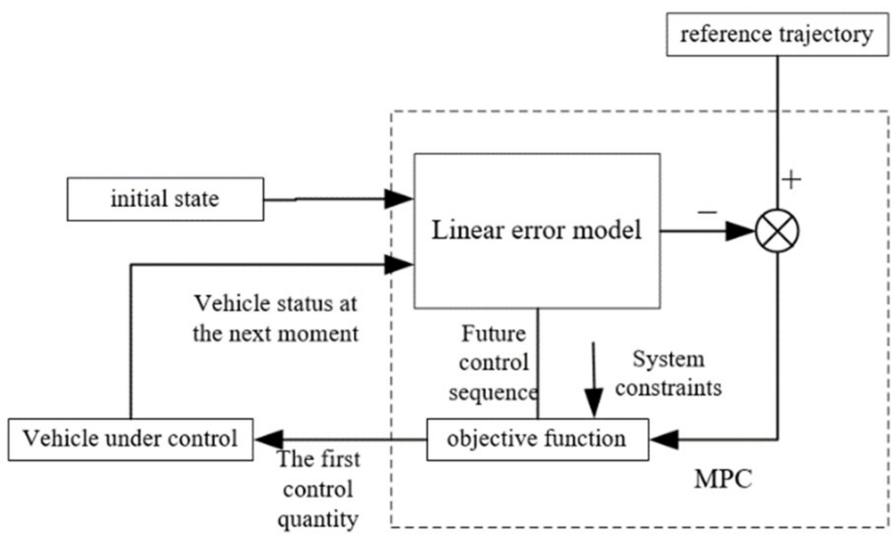
3.2. MPC Controller Design

The linear time-varying model is shown in Figure 5. In the model, the control value is initial velocity v₀ = 18 m/s; The actual measured value is v_y, r, φ, y; The control input value is α_f, ∆M_z.

Since the linear time-varying model [13] is used, it is necessary to perform linear time-varying processing and discretization processing on Equation (24).

Let A_k = I + A_T, B_k = BT, C_k = C.

where T is the sampling time, I is the identity matrix,

$$A_k=\left[\begin{array}{cccc}1-\frac{C_{cf}+C_{cr}}{m{v}_x}T& -\left(\frac{l_f{C}_{cf}-l_r{C}_{cr}}{m{v}_x}+v_x\right)T& 0& 0\\ -\frac{l_f{C}_{cf}-l_r{C}_{cr}}{I_z{v}_x}T& 1-\frac{l_f^2{C}_{cf}+l_r^2{C}_{cr}}{I_z{v}_x}T& 0& 0\\ 0& T& 1& 0\\ T& 0& v_{x}T& 1\end{array}\right]$$

(29)

$$B_k=\left[\begin{array}{cc}\frac{C_{cf}}{m}T& 0\\ \frac{l_f{C}_{cf}}{I_z}T& \frac{T}{I_z}\\ 0& 0\\ 0& 0\end{array}\right]$$

(30)

$$C_k=\left[\begin{array}{cccc}0& 0& 1& 0\\ 0& 0& 0& 1\end{array}\right]$$

(31)

So the following discrete state space equation is obtained:

$$\{\begin{array}{l}\dot{\mathit{\xi }}\left(k+1\right)=A\xi \left(k\right)+Bu\left(k\right)\\ y\left(k\right)=C_k\xi \left(k\right)\end{array}$$

(32)

In order to avoid the phenomenon of a sudden change in the control quantity of the system, it is necessary to restrict the control increment in each sampling period, so the above formula of this paper is converted and deformed:

Note: $\mathit{\zeta }=$, substitute into the above formula to obtain a new state space equation:

$$\{\begin{array}{l}\zeta \left(k+1\right)={\tilde{A}}_{\mathit{k}}\zeta \left(k\right)+{\tilde{B}}_{\mathit{k}}\mathsf{\Delta }u\left(k\right)\\ y\left(k\right)={\tilde{C}}_{\mathit{k}}\xi \left(k\right)\end{array}$$

(33)

In the formula,

$${\tilde{\mathit{A}}}_{\mathit{k}}=\left[\begin{array}{cc}{\mathit{A}}_{\mathit{k}}& {\mathit{B}}_{\mathit{k}}\\ 0_{3\times 4}& {\mathit{I}}_2\end{array}\right]$$

(34)

$${\tilde{\mathit{B}}}_{\mathit{k}}=\left[\begin{array}{c}{\mathit{B}}_{\mathit{k}}\\ {\mathit{I}}_2\end{array}\right]$$

(35)

$${\tilde{\mathit{C}}}_{\mathit{k}}=\left[\begin{array}{cccccc}0& 0& 1& 0& 0& 0\\ 0& 0& 0& 1& 0& 0\end{array}\right]$$

(36)

The optimization objective function of the path tracking and torque distribution controller is expressed as:

$$J={\displaystyle \sum _{i=1}^{N_p}{\Vert y\left(k+i\right)-y_{ref}\left(k+i\right)\Vert }^2{}_Q}+{\displaystyle \sum _{i=1}^{N_c-1}{\Vert \Delta u\left(k+i\right)\Vert }^2{}_R}$$

(37)

where y_ref is obtained by the path planning layer; Q and R are the trajectory tracking error weight matrix and the control amount increment weight matrix, respectively; N_p and N_c are the prediction time domain and the control time domain, respectively. Some parameter settings in model predictive control are shown in

Table 1. Part of the parameter settings of the controller.

Parameter Name	Value
Nc	8
Np	25
$\Delta u_{min}$	−0.02
$\Delta u_{max}$	0.2
$a_{ymin}$	−0.25 g
$a_{ymax}$	0.25 g
Q	[2000 0; 0 2000]
R	[3000 0; 0 1]

.

3.3. Torque Distribution Controller Design

Torque distribution strategy has a great impact on vehicle lateral stability. Firstly, the additional yaw moment ΔM_z output by the MPC controller is used to calculate the total demand torque T_all. Then using the proportion of the vertical load, calculates the torque of the four wheels. On the premise of ensuring lateral stability, the flexible torque distribution is realized.

The additional yaw moment ΔM_z and the four-wheel torque should satisfy the following relationship:

$$\mathsf{\Delta }{M}_z=\frac{\mathrm{b}}{2R}\left[\left(T_{Fr}-T_{Fl}\right)\cos {\delta }_f+\left(T_{Rr}-T_{Rl}\right)\right]$$

(38)

where R is the wheel radius, b is the wheel track, and T_Fl, T_Fr, T_Rl and T_Rr are the torques of the left front wheel, the right front wheel, the left rear wheel and the right rear wheel, respectively.

$$F_z=F_{z,Fl}+F_{z,Fr}+F_{z,Rl}+F_{z,Rr}$$

(39)

while:

$$\{\begin{array}{l}{k}_1=\frac{F_{z,Fl}}{F_z}\\ k_2=\frac{F_{z,Fr}}{F_z}\\ k_3=\frac{F_{z,Rl}}{F_z}\\ k_4=\frac{F_{z,Rr}}{F_z}\end{array}$$

(40)

where F_z,Fl, F_z,Fr, F_z,Rl, F_z,Rr are the vertical loads of the left front wheel, the right front wheel, the left rear wheel and the right rear wheel, respectively. Force, k₁, k₂, k₃, k₄ are the proportional coefficients of the four-wheel vertical force and the total vertical force.

According to Equations (37)–(39), the total demand torque T_all and the distributed four-wheel torques T_Fl, T_Fr, T_Rl, T_Rr can be obtained:

$$T_{all}=\frac{\mathsf{\Delta }{M}_z\cdot 2R}{d\cdot \left[\left(k_2-k_1\right)\cos {\delta }_f+\left(k_4-k_3\right)\right]}$$

(41)

$$\{\begin{array}{l}{T}_{Fl}=k_1{T}_{all}\\ T_{Fr}=k_2{T}_{all}\\ T_{Rl}=k_3{T}_{all}\\ T_{Rr}=k_4{T}_{all}\end{array}$$

(42)

The solution of the final path tracking and torque distribution controller can be expressed as:

$$\{\begin{array}{l}\min Z={\displaystyle \sum _{i=1}^{N_p}{\Vert y\left(k+i\right)-y_{ref}\left(k+i\right)\Vert }^2{}_Q}+{\displaystyle \sum _{i=1}^{N_c-1}{\Vert \mathsf{\Delta }u\left(k+i\right)\Vert }^2{}_R}\\ \mathrm{s}.\mathrm{t}.\zeta \left(k+1\right)={\tilde{\mathit{A}}}_{\mathit{k}}\mathit{\zeta }\left(k\right)+{\tilde{\mathit{B}}}_{\mathit{k}}\mathsf{\Delta }\mathit{u}\left(k\right)\\ \mathsf{\Delta }{\mathit{u}}_{\min }\le \mathsf{\Delta }\mathit{u}\left(k+i\right)\le \mathsf{\Delta }{\mathit{u}}_{\max }\\ {\mathit{u}}_{\min }\le \mathit{u}\left(k+i\right)\le {\mathit{u}}_{\max }\\ y_{\min }\le y\left(k+i\right)\le y_{\max }\\ {\phi }_{\min }\le \phi \left(k+i\right)\le {\phi }_{\max }\end{array}$$

(43)

The control quantity at time k + 1 can be expressed by the control quantity at time k plus the control increment at time k:

$$\mathit{u}\left(k+1\right)=\mathit{u}\left(k\right)+\mathsf{\Delta }\mathit{u}\left(k\right)$$

(44)

4. Simulation Analysis and Verification

The C-class vehicle model is adopted in Carsim. PD18 in-wheel motor is adopted in the motor model. According to the characteristics of the distributed drive vehicle, the vehicle parameters are shown in

Table 2. The vehicle model parameters.

Parameters	Value
Vehicle sprung mass $m_s/\mathrm{kg}$	1743
Vehicle mass m/kg	1907
Moment of inertia $I_z/\left(\mathrm{kg}\cdot {\mathrm{m}}^2\right)$	3246.9
front wheelbase $l_f$/m	1.33
rear wheelbase $l_r$/m	1.81
The height of the center of mass above the ground h/m	0.781
Wheeltrack b/m	2.029
Lateral stiffness of front wheels $C_{cf}/\left(\mathrm{N}\cdot {\mathrm{rad}}^{-1}\right)$	116,050
Lateral stiffness of rear wheels $C_{cr}/\left(\mathrm{N}\cdot {\mathrm{rad}}^{-1}\right)$	104,590

.

4.1. Verification of Co-Simulation Platform

The initial speed of the vehicle is 60 km/h, the road adhesion coefficient μ = 0.8 and the maximum value of LTR is set at 0.1. The simulation results are shown in Figure 6 and Figure 7.

It can be seen from Figure 5 that the controller can accurately track the reference path. The tracking error of the yaw angle is small, and the lateral acceleration appears slightly jittered between 0 and 1 s, but the value of the lateral acceleration is maintained throughout the process. Within a reasonable range, the front wheel corners shake slightly at 0 s to 1 s and 6 s to 7 s, but the changes in the corners are relatively gentle, and the corner values do not exceed the specified value. It can be concluded that the control effect of the controller is good and can meet the needs of vehicle obstacle avoidance.

It can be seen from Figure 6 that the value of LTR is always in a small range during the entire obstacle avoidance process, which verifies the effectiveness of the set obstacle avoidance path and meets the requirements of anti-rollover in the obstacle avoidance process.

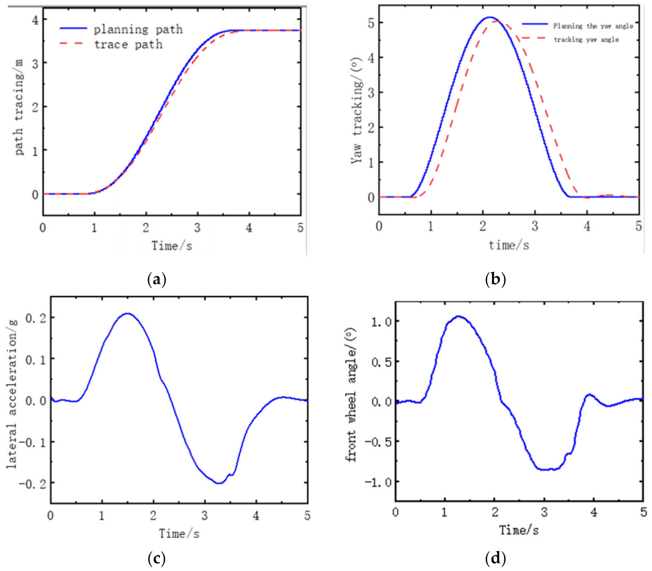
4.2. Simulation of Tracking Control Performance

The stability and robustness of the designed path tracking and torque distribution controller are verified by the simulation of different road adhesion coefficient conditions. Select high adhesion pavement coefficient μ = 0.8, low adhesion pavement coefficient μ = 0.2, μ = 0.1. The specific simulation results are shown in Figure 7 and Figure 8.

It can be seen from Figure 8a–d that the tracking control effect of the controller is excellent when the high adhesion coefficient road surface μ = 0.8. The effect is slightly decreased when the low adhesion coefficient road surface μ = 0.2, and the tracking control error is slightly increased. The changes in lateral acceleration and front wheel angle are relatively gentle under both conditions. When μ = 0.1, the vehicle deviates greatly from the planned path and the planned yaw angle. The lateral acceleration and front wheel angle also produce a lot of jitter. This is because the road adhesion coefficient is too low to the adhesion limit. Under this condition, the controller cannot perform tracking control.

It can be seen from Figure 9 that when μ = 0.8 and μ = 0.2, the vertical force changes of the wheels are relatively gentle, which meets the requirements of stable driving of the vehicle in the process of obstacle avoidance. When μ = 0.1, the tires are not sufficient to provide the vehicle with steady longitudinal and lateral force. At 2.5 s and 4.7 s, there is a large jump, which can no longer meet the stability requirements of the vehicle during driving.

Figure 10a–d shows that when μ = 0.8, the torque distribution of each wheel meets the requirements of this paper. When μ = 0.2, the torque of the left front wheel begins to increase after 1 s and reaches a peak at 1.5~3.5 s, the maximum value is 107 N∙m. The torque starts to decrease continuously at 3.5~5 s and 5~5.5 s. It reaches the reverse maximum value of 116 N∙m and then changes to 0 N∙m. The torque changes of the remaining wheels are roughly the same as the torque changes of the left front wheel, so this conclusion description will not be repeated. It can be seen that under this working condition, the controller has a good torque distribution effect. When μ = 0.1, the torque of each wheel drops rapidly to about −100 N∙m in 2 s, and the controller cannot continue to distribute the torque normally.

From the analysis of Figure 9 and Figure 10, it can be seen that the controller designed in this paper can still control the vehicle to drive according to the correct planned path under the condition of low road adhesion coefficient μ = 0.2 and carry out reasonable torque distribution, which verifies the path. The tracking controller has good robustness. When μ = 0.1, the vehicle has already slipped, and the path tracking control can not be realized.

5. Conclusions

(1)

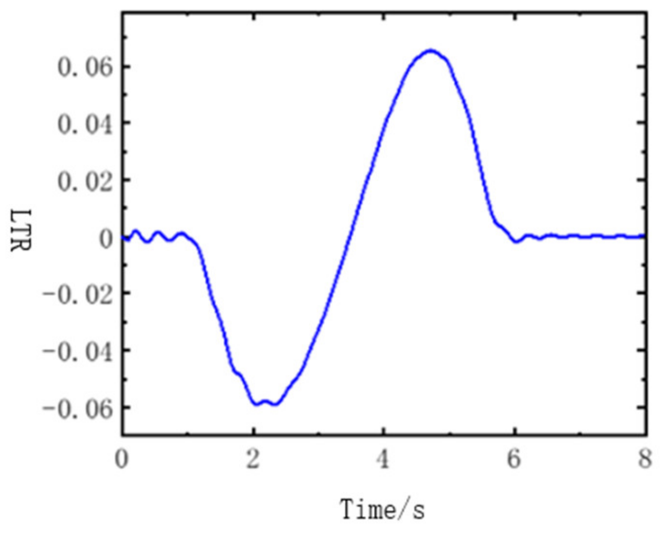
Sixth-order polynomial for obstacle avoidance path planning is presented. Through the simulation results, it is verified that the planned path can be accurately tracked, and the LTR values are always within the safe range. The vehicle has no risk of rollover. The obstacle avoidance path and tracking controller in this paper can effectively meet the requirements of safe obstacle avoidance.

(2)

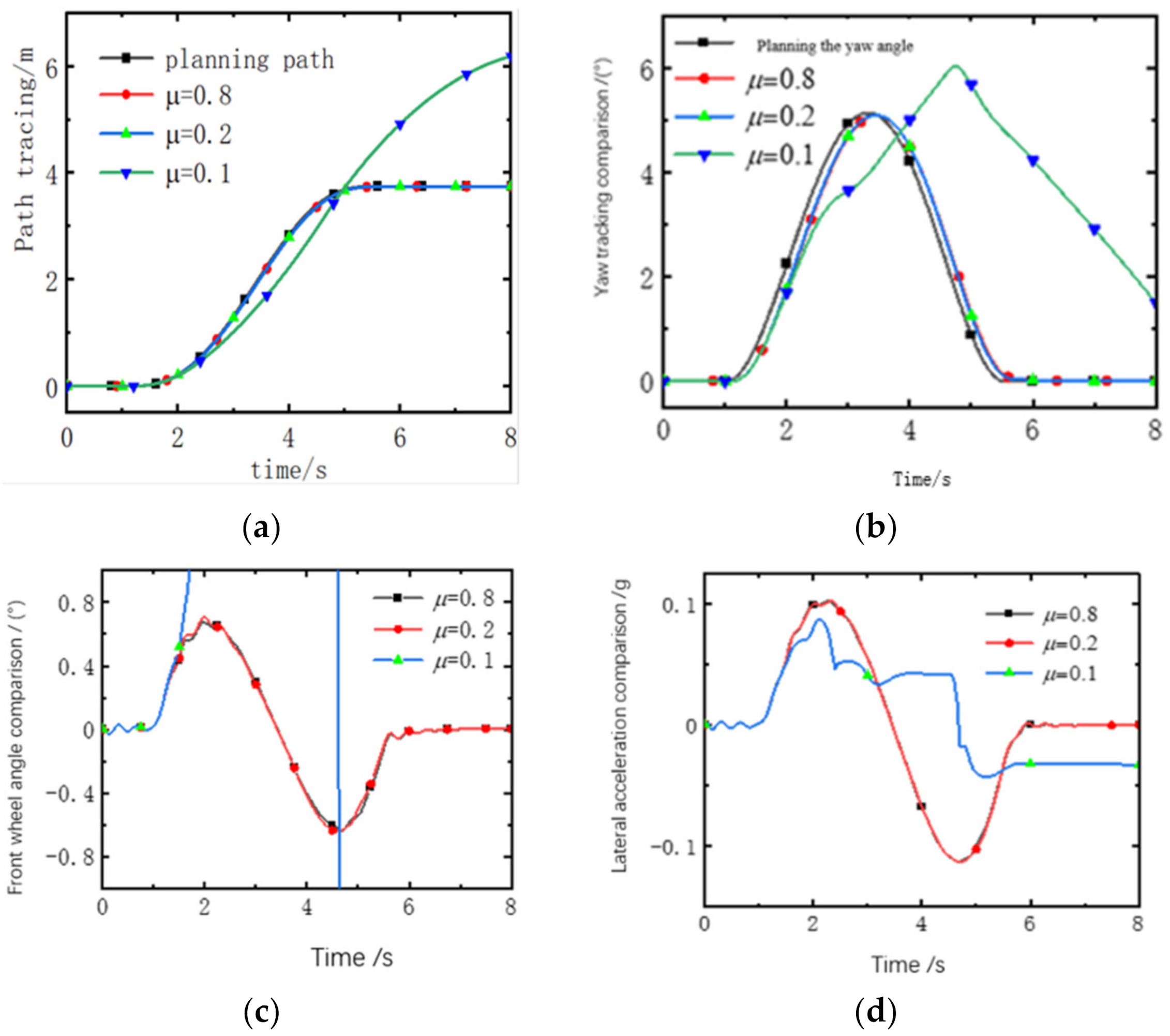
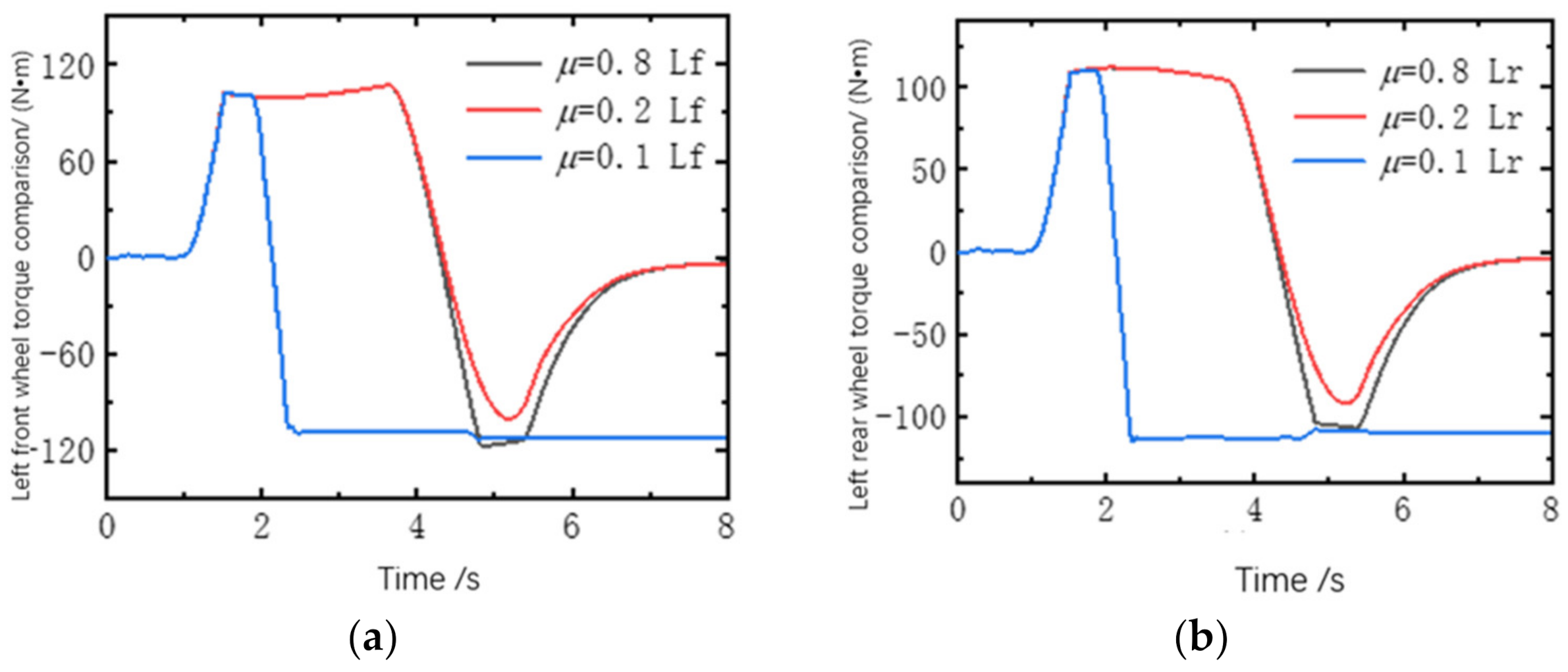
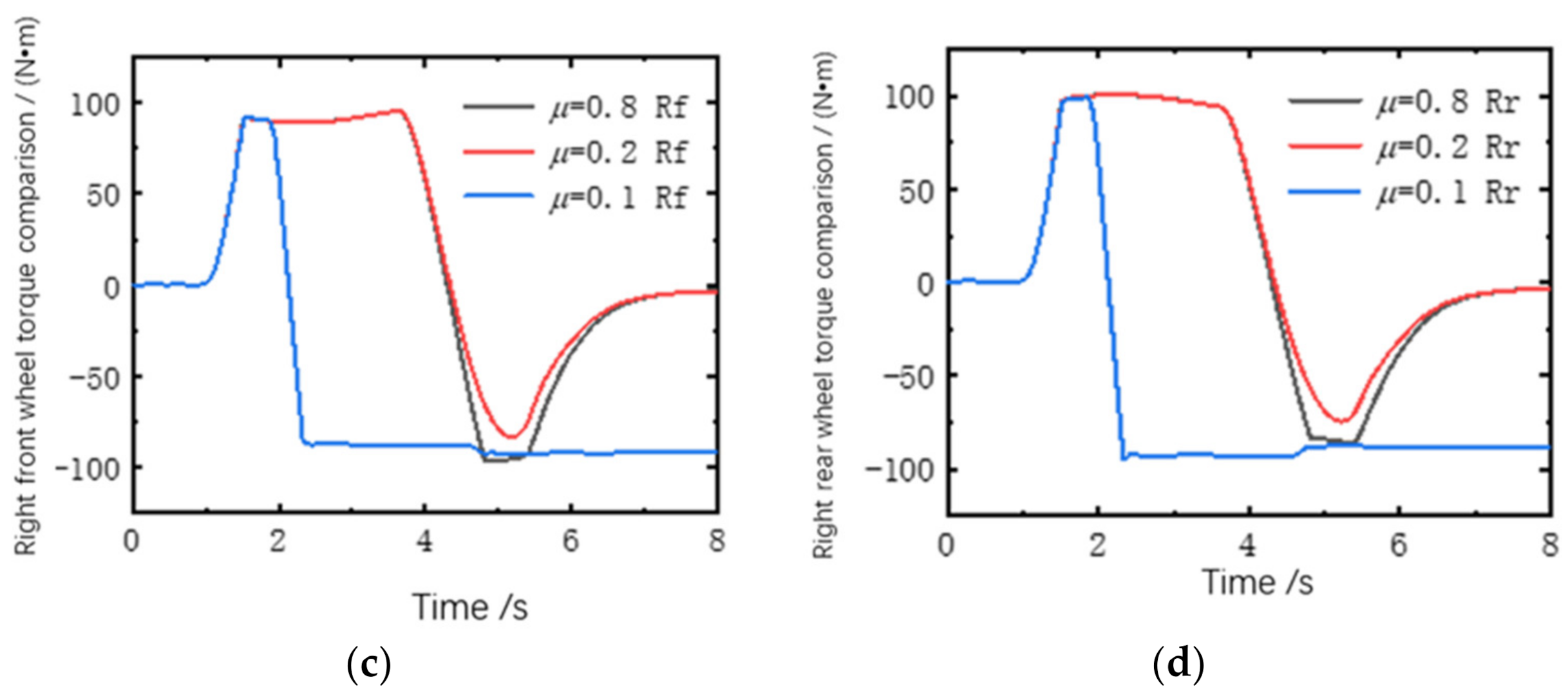
In this paper, path planning, path tracking and torque distribution are combined to achieve safe obstacle avoidance through the tracking control of the obstacle avoidance path. The path-tracking controller not only realizes the intelligent obstacle avoidance process of unmanned vehicles but also combines it with distributed vehicles. The safety and stability are improved by the torque distribution strategy in the obstacle avoidance process compared with traditional vehicles. Simultaneously, simulations are carried out under different road adhesion coefficient conditions, and the simulation results show that the vehicle can still perform safe and stable automatic obstacle avoidance under the conditions of road adhesion coefficient μ = 0.2, indicating that the controller has good robustness.

This paper provides an idea for the obstacle avoidance path tracking control of distributed drive electric vehicles. In the follow-up research work, the torque distribution controller can be improved, and better torque distribution and anti-skid control can be added to the original design scheme. The control strategy can be realized under the condition of a lower road adhesion coefficient. The real vehicle test link is added to verify the effectiveness of the control strategy in this paper.

References

- World Health Organization. Global Status Report on Road Safety 2013: Supporting a Decade of Action; World Health Organization: Geneva, Switzerland, 2013.
- Toroyan, T. Global status report on road safety. Inj. Prev. 2009, 15, 286. [Google Scholar] [CrossRef] [PubMed]
- Chang, S.; Gordon, T. A flexible hierarchical model-based control methodology for vehicle active safety systems. Veh. Syst. Dyn. 2008, 46, 63–75. [Google Scholar] [CrossRef] [Green Version]
- Guo, J.; Hu, P.; Wang, R. Nonlinear coordinated steering and braking control of vision-based autonomous vehicles in emergency obstacle avoidance. IEEE Trans. Intell. Transp. Syst. 2016, 17, 3230–3240. [Google Scholar] [CrossRef]
- Yu, Z.; Jiang, W.; Zhang, L. Torque distribution control of electric vehicle driven by four wheel hub motor. J. Tongji Univ. Nat. Sci. Ed. 2008, 36, 5. [Google Scholar]
- Chen, T.; Chen, L.; Xu, X. Coordinated Control of Path Tracking and Stability of Distributed Driving Unmanned Vehicles. Automot. Eng. 2019, 41, 1109–1116. [Google Scholar]
- Zhang, B.; Li, Z.; Shen, G. Research on intelligent vehicle track tracking based on fuzzy neural network. Automot. Eng. 2019, 41, 7. [Google Scholar]
- Wang, Y.; Chen, Q.; Gao, L. A distributed driving vehicle path tracking method based on prediction-fuzzy joint control. Sci. Technol. Eng. 2020, 20, 15100–15108. [Google Scholar]
- Hu, J.; Zhong, X.; Chen, R. Intelligent Vehicle Path Tracking Control Based on Fuzzy LQR. Automot. Eng. 2022, 44, 17–25. [Google Scholar]
- Kou, F.; Zheng, W.; Zhang, X.; Yang, H.; He, J. Path following control of unmanned vehicle using state extended MPC and corner compensation. Mech. Sci. Technol. Aerosp. Eng. 2022, 4, 1–8. [Google Scholar]
- Wu, F.; Guo, S. Intelligent vehicle path tracking algorithm based on nonlinear model predictive control. Automot. Technol. 2020, 5, 1–7. [Google Scholar]
- Li, S.; Yang, Z.; Wang, X. Trajectory Tracking Control of Intelligent Vehicle Based on T-S Fuzzy Variable Weight MPC. J. Mech. Eng. 2022, 15, 1–14. [Google Scholar]
- Zhuang, Y.; Wu, Y.; Zhang, B. Coordinated Torque Control of Distributed Drive Electric Vehicle Based on Nonlinear MPC. J. Vib. Shock. 2021, 40, 9. [Google Scholar]
- Shino, M.; Nahai, M. Yaw-moment control of electric vehicle for improving handling and stability. JSAE Rev. 2001, 22, 473–480. [Google Scholar] [CrossRef]
- Zou, G.; Luo, Y.; Li, K. Optimal distribution method of all-wheel longitudinal force for four-wheel independent electric vehicle. J. Tsinghua Univ. Nat. Sci. Ed. 2009, 49, 719–722. [Google Scholar]
- One, E.; Hattori, Y.; Muragishi, Y. Vehicle dynamics integrated control for four-wheel-distributed steering and four-wheel-distributed traction/braking systems. Veh. Syst. Dyn. 2006, 44, 139–151. [Google Scholar] [CrossRef]
- Mokhiamar, O.; Abe, M. How the four wheels should share forces in an optimum cooperative chassis control. Control Eng. Pract. 2006, 14, 295–304. [Google Scholar] [CrossRef]
- Yu, Z.; Yang, P.; Xiong, L. Application of Control Distribution Theory in Vehicle Dynamics Control. Chin. J. Mech. Eng. 2014, 50, 99–107. [Google Scholar] [CrossRef]
- Mutoh, N. Driving and braking torque distribution methods for front-and rear-wheel-independent drive-type electric vehicles on roads wit low friction coefficient. IEEE Trans. Ind. Electron. 2012, 59, 3919–3933. [Google Scholar] [CrossRef]
- Yang, B.; Zhang, W.; Jiang, Z. Simulation analysis of obstacle avoidance path planning and tracking control for intelligent vehicles. China Test 2021, 47, 71–78. [Google Scholar]
- Ren, Y.; Zheng, L.; Zhang, W. Research on Active Collision Avoidance Control of Intelligent Vehicles Based on Model Predictive Control. Automot. Eng. 2019, 41, 405–410. [Google Scholar]
- Zhang, F.; Wei, M.; Huang, L. Research on vehicle emergency lane change control based on model predictive control. Mod. Manuf. Eng. 2017, 3, 57–64. [Google Scholar]
- Gong, J.; Jiang, W.; Xu, W. Model Predictive Control for Self-Driving Vehicles, 1st ed.; Beijing Institute of Technology Press: Beijing, China, 2014; pp. 22–25. [Google Scholar]