Integration of a Chassis Servo-Dynamometer and Simulation to Increase Energy Consumption Accuracy in Vehicles Emulating Road Routes

Abstract

Electric vehicles, particularly those in mass transit systems, make use of accurate power estimations for different routes to calculate powertrain and battery requirements and plan the location and times of charging stations. Hence, chassis dynamometers are a common tool for vehicle designers as they allow for the emulation of vehicle performance and energy consumption by simulating realistic road conditions. In this paper, a method is presented where inertia events and negative slopes can be represented in the dynamometer through a single motor; allowing researchers to perform fast and cheap tests, while also considering the effect of these variables. A dynamic simulation is used to distribute the energy used in three ways: first, accelerating the vehicle by overcoming the forces opposing motion; second, emulating the kinetic energy delivered by the vehicle mass when decelerating; and third, emulating the energy delivered to the vehicle by negative slopes. Tests were carried out on a dynamometer validating the method through an example route, estimating energy consumption and regeneration; this method reduces the error in energy consumption by inertial effects and negative slopes, otherwise not considered in one motor dynamometers, showing a 9.11% difference between total test energy and real bus energy for this route.

1. Introduction

Electric mass transit vehicles have become an attractive alternative in population centers to provide mobility options with positive effects on the livability of cities; this is because they reduce pollution by not using fossil fuels and are quieter than their internal combustion counterparts [1,2,3]; however, massive implementation of electric vehicles (EV) has technical limitations that are being solved day by day, and they are mainly: the weight per kWh of stored energy ratio; the cost per kWh of energy [4]; the impact of battery charging cycles [5]; and the infrastructure required for energy charging [6] and the impact on energy distribution networks [7]. Alternative strategies to the use of batteries have been explored such as the use of contact supply cables along the track [8], battery exchange systems [9], wireless charging systems [10,11] or the implementation of electrified roads (e-roads) [12]; these systems present even higher investment, assembly, and maintenance costs than conventional electric bus systems [13,14,15] which limits their adoption.

Mass transit lines usually have established routes and hours, which is why it is possible to plan a battery charging system to maintain the highest possible uptime of the service [16,17,18]; this is one of the reasons why public transport operators are increasingly opting for tailor-made solutions that guarantee the highest energy efficiency per passenger [19,20]. Among the tests performed, those of fuel or energy consumption have become particularly prevalent with the existing global urgency to reduce CO₂ emissions [21,22]. For example, Hu et al. conducted an analysis two different energy management strategies and battery sizes, where smaller batteries represented less energy consumption by fewer passengers carried as system uptime decreased [23]. Kivekäs et al. numerically evaluated six different bus models analyzing their driving cycle and passenger load sensitivity, where aggressive driving was found as the main factor in increasing energy consumption [24]. Not surprisingly, Perger et al. conclude topography has the greatest impact on public transport routes, where the shortest route possible is often not the most efficient, either in passenger distribution (amount of passengers transported) or energy required per passenger [25]. Most of these studies comment on the impossibility of reaching a general design solution which is optimal for the different topographical, climatical and passenger requirements within different cities and even different routes within the same city.

There are multiple other effects that require consideration to reach these efficient designs, for example, speed differences within and between routes [26]. Many of these studies make use of field tests with the vehicles to estimate energy consumption and ecological aspects for different designs and operating conditions [27,28,29,30]. Other factors, such as the use of heating systems have proven to increase energy consumption up to 64.5% in the winter time, where tests where performed by driving four different electric vehicles in 3 different times of the year (fall, winter and spring) [31]. Other types of tests have been conducted by equipping buses currently used for mass transit in the city of Beijing with pollutant emission detection systems, where rapid accelerations were found to have the greatest impact on emissions and energy consumption [32]. Furthermore, simulation and dynamometer tests have been validated through real vehicle driving, where once again, the slope effect appears to have the biggest impact in energy consumption as shown by Beckers et al. [33]. Because of the capability of properly representing these conditions, the automotive industry uses vehicle dynamometers to evaluate the power train from the batteries to the wheels, with the purpose of simulating specific operating conditions by means of route variables (slope, speed, load/passengers) [34] and control variables (environmental, road condition, traffic) [35,36].

These dynamometers may vary drastically in their components and operation based on the particular needs of each vehicle manufacturer or research institution [37]. Amongst the different types of dynamometers used, this research focuses on those where the entire vehicle powertrain (often with chassis and cabin) is placed on rollers to simulate driving conditions. Mayyas et al. published a review of these types of dynamometers classifying them according to the adhesion/mounting of the vehicle to the dynamometer [38]; this type of dynamometer has been widely used for decades [39,40,41,42,43] being subject to changes and improvements, largely, in how vehicle inertia is represented. Traditionally, this was performed by means of discrete disks used as a flywheel to store the kinetic energy; however, many modern dynamometers use an auxiliary motor to emulate inertia or downwards slopes [44,45]; these assemblies are generally used after the initial stages of the design process, where it is desired to accurately evaluate a wide variety of component combinations quickly [46,47]. The use of dynamometers and other technologies has allowed the automotive industry to reduce vehicle design and production from upwards of 10 years, to as little as a few couple years [48].

The need for an even quicker means of testing is one of the reasons why numerical simulation becomes relevant to rapidly evaluate solutions; these studies usually fulfill the function of evaluating many components and route conditions at a much lower cost and time than route or dynamometer tests through the use of iterative or analytic methods performed in virtual environments [49,50,51]. Studies in this area are varied, for example, Bottiglione et al. simulate and compare electrical buses with different types of transmissions [52]; Xu et al. propose methodologies for simulating traffic and driving styles [53]; while Fiori et al., propose an instant speed and acceleration analysis in order to estimate electric vehicle energy requirements [54]; however, authors of these different studies, and many others focused on mathematical simulation, comment on the limitations of using theoretical models for precise component interaction analysis. For vehicle components selection simulation software may be sufficient; however, components and systems combinations are usually tested on a dynamometer to guarantee the desired performance while accurately evaluating diverse route and driving conditions [55].

This paper presents a method to emulate the different events present on the road through the systemic integration of a servo-dynamometer and the power train of the vehicle to be tested. The purpose is to integrate mathematical simulation elements with a dynamometer to emulate electric vehicle operation, allowing for energy consumption tests of real routes with a simple assembly of a single motor and brakes. The method aims at emulating powertrain efficiency using the test-bench while simulating inertia and negative slopes. In Section 2, the mathematical model of the vehicle and the dynamometer to be used for vehicle representation will be introduced. Afterwards, a strategy is proposed for representing vehicle dynamics using a one motor dynamometer. The motor is operated either as part of the dynamometer, providing inertia and slope torques; or the vehicle motor, providing the torque required for bus movement. The simulation algorithm is then presented, as is the dynamometer used for model validation. Section 3 presents the results obtained in terms of evaluating the mathematical model by representing a small route segment in which a vehicle covers the distance between two possible bus-stops in a hillside city. Section 4 presents the discussion of the results obtained considering how the method improves the existing one motor options. Finally, Section 5 concludes with a summary of the method while also discussing its limitations.

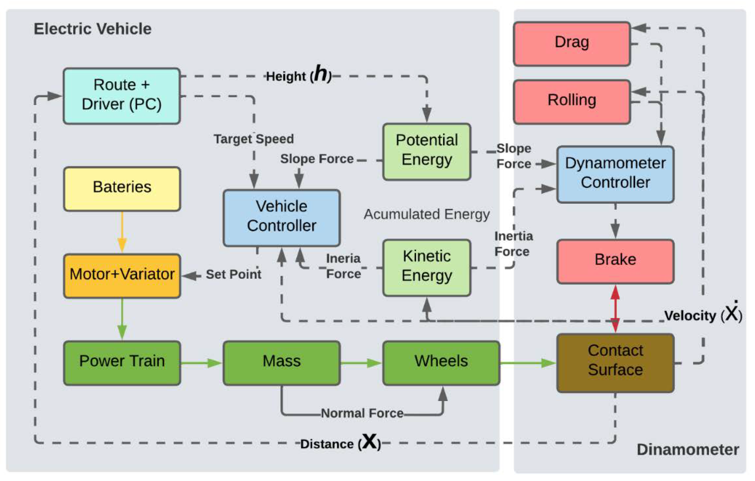
2. Materials and Methods

The vehicle in a servo-dynamometer is not under the same conditions as one on the road as it does not accumulate kinetic energy or gravitational energy; therefore, they must be represented to properly evaluate route performance. In this section, vehicle and dynamometer operation are compared, emphasizing the way to distinguish energy used by the vehicle’s engine on the track and the total energy required to conduct the tests. Afterwards, the mathematical models of the vehicle and the dynamometer are presented. Finally, the proposed simulation methodology is described.

A free-body diagram of the vehicle accelerating uphill is shown in Figure 1. The forces and torques to which the vehicle system is subject on the road are: motor driving force ($F_m)$, gravitational force $(F_g)$; rolling resistance forces $(F_r)$; aerodynamic drag force $(F_d)$; inertia forces $(F_i)$ of the vehicle; inertial torques $(T_i)$ of rotating elements; torques due to the motor $(T_m)$ propelling the vehicle; torques due to vehicle brakes $(T_b)$; negative torques due to friction between transmission elements; transformations of torques traveling from the engine to the wheels; and, conversion of rotational to linear motion at the wheels (a full list of expressions is provided in Appendix A). Of these forces and torques, some are always negative, such as rolling or aerodynamic drag; however, the gravitational force and inertial torques are constantly changing according to the dynamics of the vehicle and the characteristics of the route being emulated. Therefore, the dynamometer roller is provided with a device that provides negative torque, a servo brake, and one that provides positive torque, a servo motor.

This paper presents a methodology to use the engine of the vehicle being tested with a double functionality: first, to propel the vehicle to overcome the forces and torques imposed by the road, and second, to provide the torque that emulates the forces and torques due to gravity and inertia. Proper energy separation, between actual vehicle consumption and the emulation of other torques, is necessary. To achieve this objective, the energy provided by the battery is not counted in one counter but in three:

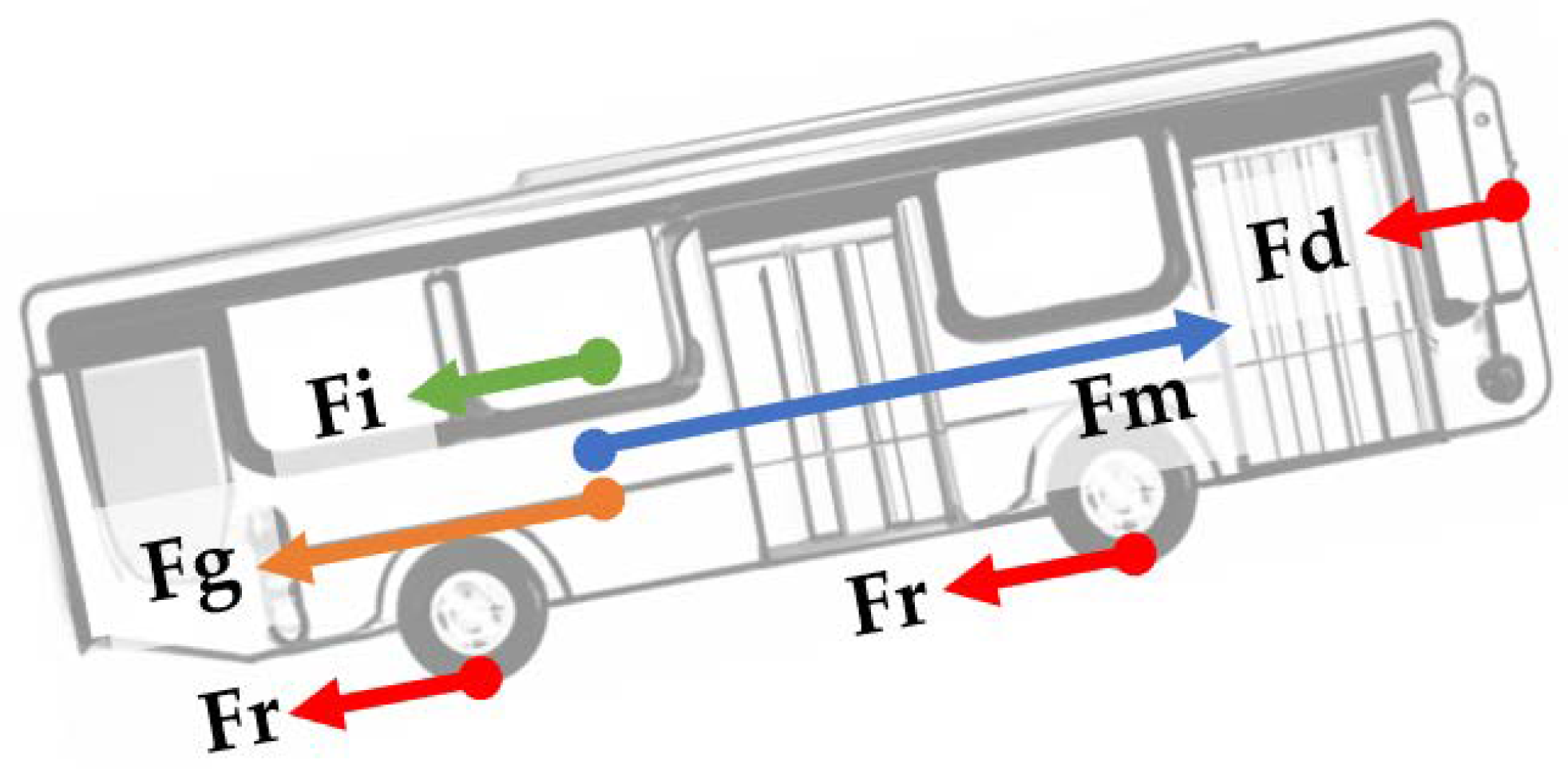
• Energy used by the motor to carry out the tasks of transportation.
• Energy used to turn the wheels of the vehicle when the vehicle is going down a slope pushed by gravity.
• Energy used to turn the wheels of the vehicle when the driver’s command is to cut the motor’s energy. At this point, the mass of the vehicle and the rotating masses have stored kinetic energy and release it; however, in this method, only linear masses are considered.

In cases two and three, one motor dynamometers simulate these effects through the same motor used for accelerating (case one), thus energy used to reach and maintain target speeds is different than that of actual bus operation. Furthermore, in actual vehicle operation kinetic and potential energy stored in the vehicle enter the powertrain directly to the wheel; this means that the energy required to represent these effects by the vehicle motor is greater, as it needs to be transported from the motor to the wheel with the respective vehicle efficiency. On some occasions the types of power consumption will overlap; therefore, the vehicle and dynamometer are operated using a variable structure for the control algorithm; this structure is divided into three levels (negative, positive, constant or no change) for both factors (speed change and slope). The different operating conditions or structures that the dynamometer emulates are shown in Figure 2.

This method does not consider reversing because it is relevant in terms of maneuvering, but not in terms of consumption, particularly in public transit routes. Although constant speed or slope could be included within their negative counterparts, their consideration as neutral is useful for simulation purposes reducing the complexity of operations.

Table 1. Variable structure for determining sources of work.

	Decelerating	Constant Speed	Accelerating
Flat	Work (EV Sim) Braking (EV Sim) Regeneration (EV Sim) Inertia (EV Sim)	Work (Motor)	Work (Motor) Inertia (Motor)
Uphill	Work (EV Sim) Braking (EV Sim) Regeneration (EV Sim) Slope (Motor) Inertia (Motor)	Work (EV Sim) Slope (Motor)	Work (Motor) Inertia (Motor) Slope (Motor)
Downhill	Braking (EV Sim) Regeneration (EV Sim) Inertia (EV Sim)	Braking (EV Sim) Regeneration (EV Sim)	Work (EV Sim) Braking (EV Sim) Regeneration (EV Sim) Inertia (EV Sim)

shows this relationship between the different sources of work, both to propel the bus and to stop it. There are multiple cases where it is necessary evaluate the vehicle dynamics before determining how torque flows within the powertrain. For example, a driver on a downhill segment is likely to accelerate up to the target speed and then allow the bus to roll freely or may even have to brake slightly to maintain a constant speed. For this stretch, the work to accelerate the mass of the vehicle is done partly by the bus motor and partly by the slope; then, to maintain its speed the slope does most if not all the work.

2.1. Vehicle Mathematical Model

In this section we present the mathematical model of an electric vehicle which will be used all throughout our algorithm to calculate the forces and torques to be represented. For calculation purposes all torques and forces are analyzed at the wheel, where the resultant force or $F_w$ as shown in Equation (1), is equivalent to the bus’s force as experimented by the chassis and cabin:

$$F_r+F_d+F_g+M\frac{d\dot{x} }{dt}={{\displaystyle \sum }}^{ }F=F_w$$

(1)

The rolling forces and aerodynamic drag are determined by vehicle components and chassis and the gravitational and inertial forces by its operating conditions; their respective models will be presented in the following section. The relationship between the linear moving elements (bus mass), to the torque of the rotating elements (e.g., motor and powertrain), are shown in Equations (2) and (3); these expressions are used to obtain forces and speeds at the wheel from their torque and angular velocity counterparts. With $r_w$ as the wheel radius and ${\dot{\theta }}_w$ as the angular speed of the wheels. The torque sum on the wheel in terms of motor torque is show in Equation (4). Where ${\eta }_t$ is the transmission efficiency; $R_r$ as the torque relation between motor and wheel (given by $\dot{{\theta }_m}/\dot{{\theta }_w}$); $I_m$ y $I_w$ as the inertia moments of elements on the motor side of the transmission and wheel side of the transmission; and $\dot{\theta }$ as their respective angular speeds.

$$T_w=F_w\times r_w$$

(2)

$${\dot{\theta }}_w=\frac{v_v}{r_w}$$

(3)

$$T_m\times {\eta }_t\times R_r+I_m\frac{d\dot{{\theta }_m} }{dt}\times {\eta }_t\times R_r+I_w\frac{d\dot{{\theta }_w} }{dt}+T_b={{\displaystyle \sum }}^{ }T=T_w$$

(4)

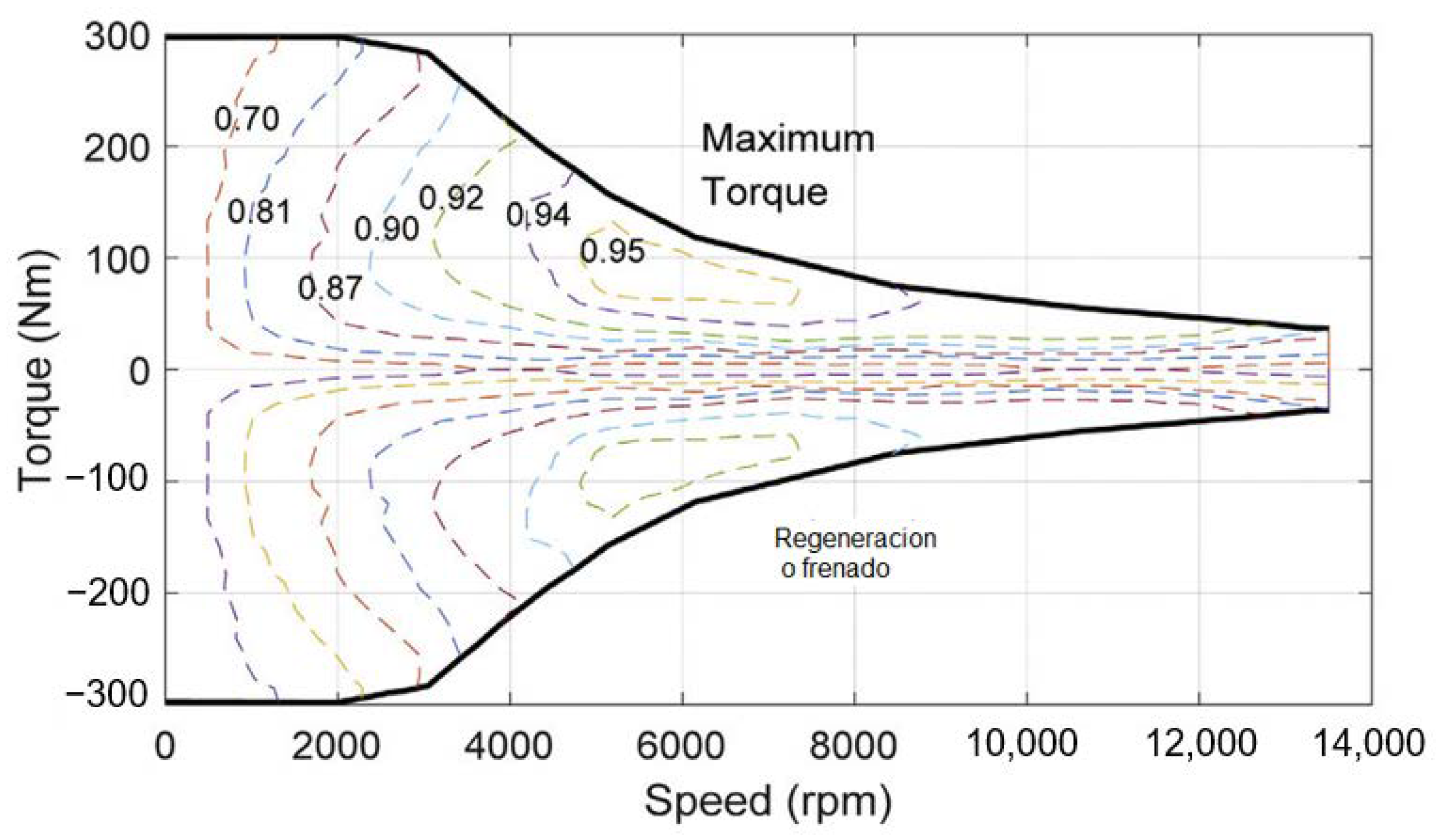
2.1.1. Speed Control

The motor torque, Equation (5), is obtained from the throttle actuation percentage, %γ, shown in Figure 3 as the proportion of available power employed. The maximum torque line is available only for brief periods of time before damaging the motor, thus %γ represents an operation point somewhere between 0 (no throttle) and the continuous torque line (100% throttle). Motor angular speed, $RP{M}_m$, is used to determine the horizontal coordinate within the efficiency map; while the respective efficiency, ${\eta }_m$, is determined by $RP{M}_m \mathrm{and} \%\gamma$.

$$T_m=f \left(\%\gamma , RP{M}_m, {\eta }_m\right)$$

(5)

$$\%\gamma =f\left(v_{vr}, X_i,t_i,{\beta }_1,{\beta }_2,{\beta }_3,{\beta }_{4,} \tau \right)$$

(6)

The throttle percentage, $\%\gamma$, is a complex function shown in Equation (6) that the driver adjusts according to its parameters which are described in order of appearance: (1) $v_{vr}$: The ratio between vehicle speed and the reference speed for current segment of the route; if the route is in good conditions, straight and with no traffic, $v_{vr}$ increases and vice versa. (2) $X_i$: is the current distance traveled. (3) $t_i$: time elapsed since the start of the route. If the time is short in relation to the expected value for this position ($X_i$) in the route $\%\gamma$ decreses and viceversa; this speed set-point and difference to the expected location are constructed using a multi-variable PID that generates both positive and negative throttle values. Parameters 4 to 7 ($\beta$ parameters) are route characteristics which modify the PID output as speed reductions: ${\beta }_1$ indicates whether the vehicle is approaching a regular stop or a traffic light. ${\beta }_2$ indicates the presence and distance of vehicles in front. ${\beta }_3$ indicates a passenger’s request to stop. ${\beta }_4$ indicates varying road conditions: humidity, sand on the road, visibility, etc. Parameter 8, $\tau$, indicates the driver’s personality: calm, fast, aggressive, and may be used for PID configuration, in the form of acceleration and braking ramps or actuation delay. Further $\beta$s may be added as required by designers to represent different road conditions which are of interest, such as the weather (rainy, dry, snow), or temperature.

2.1.2. Braking

The driver operates the brakes of the vehicle by generating a torque $T_b$ as shown in Equation (7), whenever the target speed is lower than the current speed, while also depending on the different events, βs, described above as shown in Equation (8).

$$T_b=f \left(\%{\gamma }_b\right)$$

(7)

$$\%{\gamma }_b=f\left({\beta }_1,{\beta }_2,{\beta }_3,{\beta }_{4,} \tau \right)$$

(8)

The brake converts the kinetic energy from the mass in motion into electrical energy (regenerative braking), thermal energy (traditional braking), among others; it is assumed that in electric vehicles a certain percentage of braking is performed by the motor and results in regenerative braking ($T_{brg}$); therefore, this torque is obtained as a function of the motor RPM (and the available negative torque for this RPM) and the %set adjustment of braking torque made to the motor control as shown in Equation (9). For example, 0–30% of the brake pedal travel may be assigned exclusively to regeneration and thereafter braking is made as a combination of both types of braking, up to 100% of available braking torque.

$$T_{brg}=f\left(RPM, \%{\gamma }_b, \%set\right)$$

(9)

When regeneration is being evaluated, regenerative torque $T_{brg}$ is subtracted from the torque $T_b$, and the regenerated energy is calculated. The amount of energy regenerated depends on the efficiency of the vehicle’s powertrain, motor, inverter, and the ability to store the energy in the batteries. In this method a mirrored efficiency map, as show in Figure 4, is used to calculate motor regeneration for negative torques. In our implementation efficiencies are calculated instantaneously from dynamometer sensors; however, a custom efficiency map obtained, which may prove more accurate than assuming that positive torque efficiencies are equivalent to those of negative torques used for regeneration.

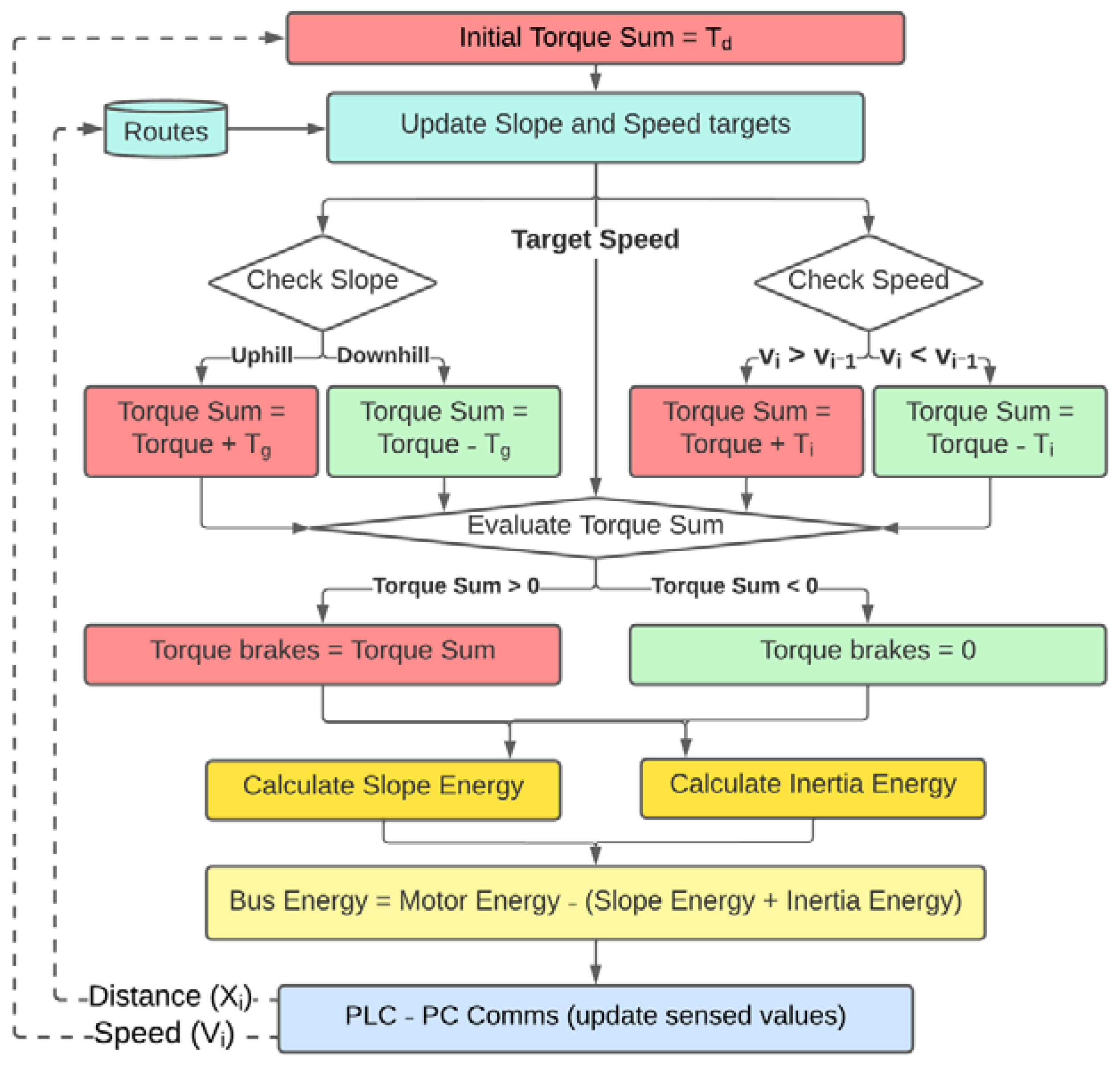
2.2. Dynamometer Mathematical Model

The torque to which the vehicle is subjected on the dynamometer is given by expression Equation (10). With $a_v$ as the linear acceleration of the vehicle, $v_v$ vehicle speed as measured by dynamometer sensors, $\alpha$ as the angle of inclination of the route, ${\dot{\theta }}_m$ as motor angular speed, ${\dot{ \theta }}_w$ wheel angular speed, and $\mathsf{{\rm M}}$ as the rolling coefficient of the road in relation to that of the dynamometer.

$$T_{dyna}=f\left(a_v, v_v, {\dot{\theta }}_{m,}{\dot{ \theta }}_w, \alpha , \mathsf{{\rm M}}\right)$$

(10)

The forces and torques that the dynamometer must emulate correspond to our representation of the vehicle on the track and they are $T_d$ as the aerodynamic drag torque; $T_r$ as the rolling torque; and $T_g$ as the gravitational or slope torque; their values are calculated before actuation, through either motor or brakes, using Equations (11)–(13), using $r_w$ to transform the respective vehicle forces into torques.

$$T_d=r_w{F}_d=r_w\frac{1}{2}\rho C_{d}A{\left(v_v\right)}^2$$

(11)

$$T_g=r_w{F}_g=r_w m g\sin \left(\alpha \right)$$

(12)

With $\rho$ as air density; $C_d$ as the drag coefficient and A as the front area of the vehicle. For vehicle tests on flat highways, the relative wind-vehicle speed, and the angle between the two are analyzed as the variable drag coefficient according to the Reynolds number. In addition to the aerodynamic force, the brake also simulates $T_r$ (Equation (13)), as a function of its difference from that of the dynamometer; and $T_g$, with $m$ as the mass of the vehicle.

This method evaluates bus rolling $T_r$ as a function of vehicle mass $m$, tire pressure $P_w,$ and rolling coefficient $R$ as shown in Equation (14). Dynamometer friction, $T_{rd}$ is a function of angular velocity $f\left({\dot{\theta }}_m\right)$, and is composed of static and dynamic friction components which depend solely on the RPM and must be determined by operating the dynamometer without any braking for all ranges of available RPMs. The torque measured by the sensors at constant speed for every RPM corresponds to dynamometer friction torque. The method compares $T_r$ and $T_{rd}$ applying only the difference between expected vehicle rolling and actual dynamometer rolling.

$$T_r=f\left(m, P_w, R\right)$$

(13)

After determining the dynamometer’s rolling its inertia is also calculated by cold-start to max-RPM accelerations. In Equation (14), dynamometer speed change over time and motor torque, $T_m$, are measured and $T_{rd}$ is known from the previous characterization, allowing for the calculation of $I_{dyna}$. For this calculation ${\dot{\theta }}_{dyna}$ represents the angular speed of the elements on the side of the main transmission. Otherwise, it might be assumed that $T_{rd}=T_r$ and that vehicle rotational element’s inertia and dynamometer’s inertia are similar, thus requiring no calculations as the effects are properly represented in the dynamometer. Such simplification is possible as powertrains should be similar if not equal for both dynamometer and evaluated vehicles, while rolling between the wheel and road or contact surface may be calibrated through means of contact-surface tensioning, tire pressure or other equipment.

$$T_m=T_{fr}\left({\dot{\theta }}_m\right)+I_{dyna}\frac{d{\dot{\theta }}_{dyna} }{dt}$$

(14)

2.2.1. Energy Counting

The torque used by the motor to simulate negative slopes with speed change is given by Equation (15). While the torque used by the motor to simulate inertia is given by Equation (16). Subindex i and g in the torque denote it’s the portion of motor torque corresponding to inertia and slopes respectively.

$$m g\sin \left(\alpha \right)=\frac{1}{r_w}\left[T_{mg}\times R_r\times {\eta }_t+R_r I_m\frac{d\dot{{\theta }_m} }{dt}+I_w\frac{d\dot{{\theta }_w} }{dt}\right]$$

(15)

$$m\frac{\mathsf{\Delta }{v}_v}{\mathsf{\Delta }t}=\frac{1}{r_w}\left[T_{mi}\times R_r\times {\eta }_t+R_r I_m\frac{d\dot{{\theta }_m} }{dt}+I_w\frac{d\dot{{\theta }_w} }{dt}\right]$$

(16)

The motor energy counter evaluates discretely for every $\mathsf{\Delta }t$ (given by iteration time), using the values measured by machine sensors ($\dot{{\theta }_m}$, $T_m$) as inputs for Equation (17). Energy consumption or regeneration is later added for all segments, as shown in Equation (18), from which energy required for any route or specific route segment may be calculated.

$$\mathsf{\Delta }E=\left(T_{mg}+T_{mi}+T_{dyna}+T_r \right)\times \dot{{\theta }_m}\times \mathsf{\Delta }t$$

(17)

$$E={\displaystyle \sum }_{i=0}^{i=i_n}\mathsf{\Delta }{E}_i$$

(18)

Figure 5 shows powertrain components, dynamometer components and their interactions. The energy flows (solid lines) are torques and forces applied to the vehicle on the dynamometer, while information flows (dotted lines) are simulated within the control and their effects are represented through dynamometer motor or brakes. Thus, physical representation and simulation components are integrated. Energy is accumulated in the form of height and speed, in relation to vehicle mass, as seen from the light green boxes. While light red boxes represent non conservative forces and are applied through the brake. Velocity and torque calculations are made at the wheel; hence velocity and distance lines start from it and feed control components in blue after being processed.

2.2.2. Virtual Route Recreation

The inputs required for this methodology are the topography of the route (particularly the slope and the condition of the road), vehicle target speed and the number of passengers according to the distance traveled. The stops along the route and other route characteristics, such as speed reductions, bus stops, among others are included as the $\beta$s mentioned in Section 2.1.1; these are entered as an array where the route is split into different segments which represent the changing road characteristics mentioned before. Segment length may vary in order to adequately represent the changing characteristics of the route being studied. Route information may be collected in-situ, reconstructed from GPS, satellite, drone survey or even constructed through manual or simulated inputs. Information for a particular bus route in these hillside city environments in shown in Figure 6.

2.3. Emulation on the Dynamometer

From the route information, the driver uses Equations (6) and (8) to actuate the vehicle’s motor and brakes. Then, the dynamics of the vehicle on the wheel are evaluated using vehicle Equations (1)–(9) and the dynamometer Equations (10)–(16). The difference between the torques to which the dynamometer and the vehicle are subjected is obtained; this resultant force, $F_{dyna}$, (or dynamometer force), when opposing the movement of the vehicle is applied by means of the dynamometer, as vehicle force is correctly represented by ${{\displaystyle \sum }}^{ }{F}_v\approx F_{dyna}$. When a negative torque is to be simulated the brakes are left unoperated and thus $F_{dyna}$ is equal to zero.

Afterwards, based on the driver’s personality (e.g., how fast the driver wants to reach his target speed) and route information a new target speed for the bus is obtained. Equation (19) is obtained from Equation (1) by incorporating the bus and dynamometer relations and is used to evaluate inertia for the vehicle and adjust controller velocity considering the represented conditions.

$$F_i=M\frac{d\dot{x} }{dt}=M\frac{{\dot{x}}_i-{\dot{x}}_{i-1}}{t_i-t_{i-1}} =F_{rd}+I_{dyna}\frac{d\dot{{\theta }_d} }{dt}+F_{dyna}+F_m$$

(19)

Slope and inertia energy are calculated through Equations (15) and (16) and their value is subtracted from the total energy used as measured from the dynamometer sensors. Energy used can be measured either as voltage and current between batteries and variator (electrical power) or torques and angular speeds at the motor (mechanical power), depending on the instrumentation available. Figure 7 shows the operation algorithm used to control the dynamometer and for energy consumption calculation; red squares represent torques that oppose movement, green squares those that propel the vehicle forward, yellow squares energy calculations and blue and cyan squares represent control and communication operations.

Model Evaluation with Dynamometer Tests

A dynamometer with the characteristics described in previous sections (rollers, belt, and a single motor), and shown in Figure 8, was used to simulate the different operating conditions. A windows computer with Labview (version 2020, National Instruments (NI), Austin, TX, USA) was used to read route files from excel spreadsheets which contained segment information. LabVIEW was also used to simulate the driver and conduct energy and braking calculations; iteration values for acceleration and braking were sent to the PLCs via Modbus. Two PLCs were used, one for the vehicle and one for the dynamometer, which conducted motor and brake operation, sensor readings and controlled other subsystems such as refrigeration and emergency brake release or battery disconnection. The computer saved instantaneous energy and other sensor readings for each iteration in an excel file which was later processed in Python (version 3.9.3, Python Software Foundation, Beaverton, OR, USA) for total energy calculations.

Powertrain and dynamometer components are listed as follows: (a) Motor—HPEVS AC-20-03.27.8. Maximum torque: 173 Nm. RPM range: 0–8000 RPM. (b) Driver: HPEVS Curtis 1238e-7621 Controller. Connected to a 96 V DC battery pack. Maximum current 650 Amp; (c) Continuously variable transmission (CVT), Drive Pulley—Polaris^® (Medina, MN, USA) Primary Drive Clutch for Sportsman 500. Driven Pulley—Team^® (Audubon, MN, USA) Tied Clutch Arctic Cat Pro Chassis reference 421896. Belt—Gates^® (Denver, CO, USA) 4430V560 Multispeed; (d) Torquemeter—Galoce^® (Xi’an, China) GTS100 Dynamic Torque Sensor. Torque range 0–150 Nm. (e) Torquemeter—Forsentek^® (Shenzhen, China) Rotary Torque Sensor fyd. Torque range 0–1000 Nm, not shown in this image. (f) Gearbox: 40-97001-3, Flowfit, relation: 3.8:1; (g) Wheels and contact surface; (h) Brakes and Compressor: Minimum brake pressure (each): 0.2 atm/Minimum brake torque: 0.9 Nm; Maximum brake pressure: 8 atm/Maximum brake torque: 1400 Nm.

A test route corresponding to a 200 m stretch from one stop to another (e.g., no passenger change) was used to analyze the method’s results, as shown in Figure 9; this type of route corresponds to hillside cities where urban or suburban buses travel short lengths within stops (100–300 m) with varying slope and road conditions; this test route was chosen as it displays a downhill segment starting from rest, where the bus brakes to stay close to the target velocity of the segment as the driver has a speed reduction event β in the form of a speed bump. The slope increases slowly until reaching positive values which coincide with the greatest positive inclination. Afterwards, the driver coasts for the rest of the route until decelerating near the end, close to the next stop.

3. Results

We present the test route to be analyzed from which three different types of interactions between torques are shown. In the following figures, the x axis shows the number of iterations (i) corresponding to the update of the sensors and actuators values, where the time (dt) between iterations is 0.5 s; this test lasted for a total of 2:04 min where 206 m are covered. There is only one stop at the end of this segment, as the route describes a segment of continuous bus operation; therefore, there is no passenger hop-on or off the dynamometer simulates a mass of 1200 kg during the whole test.

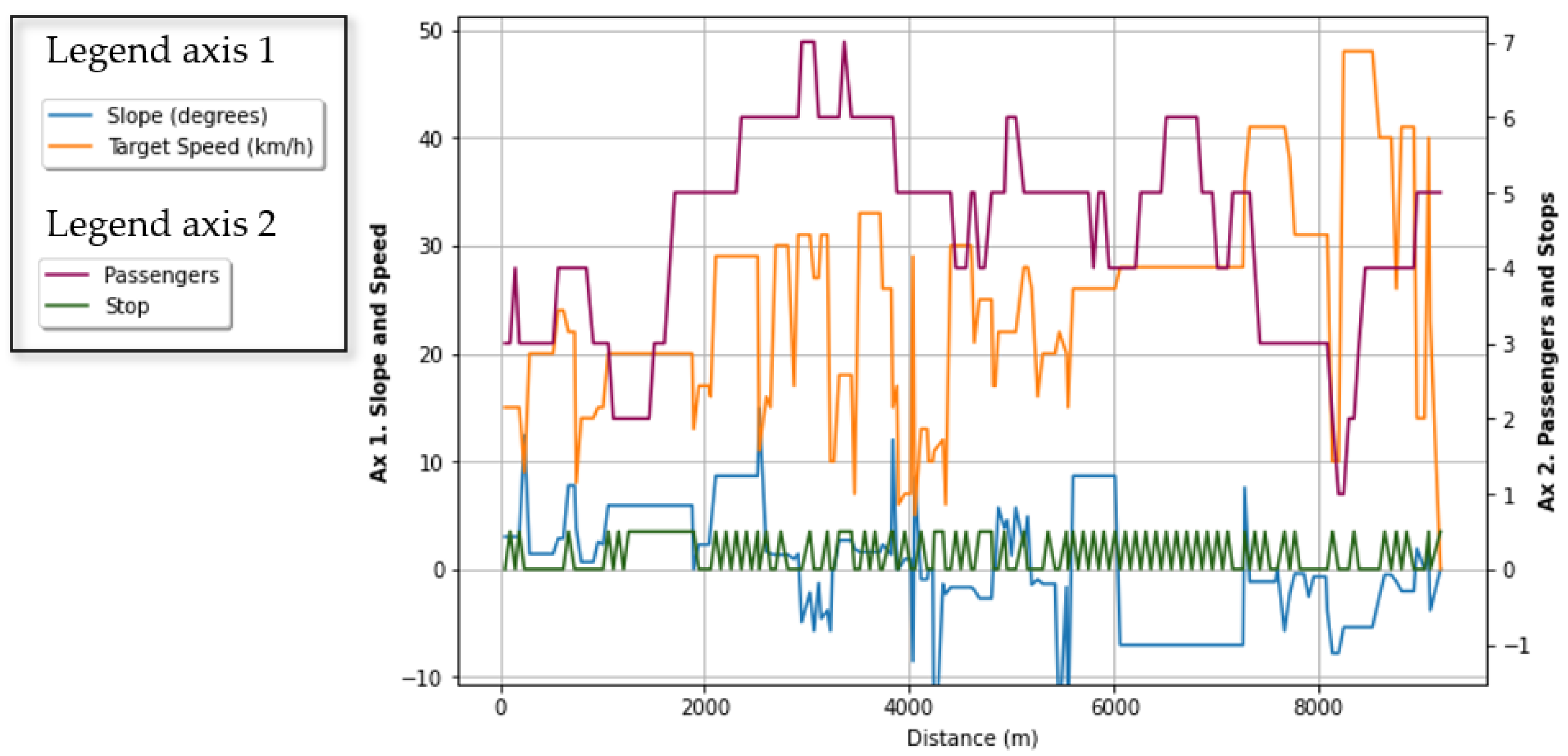
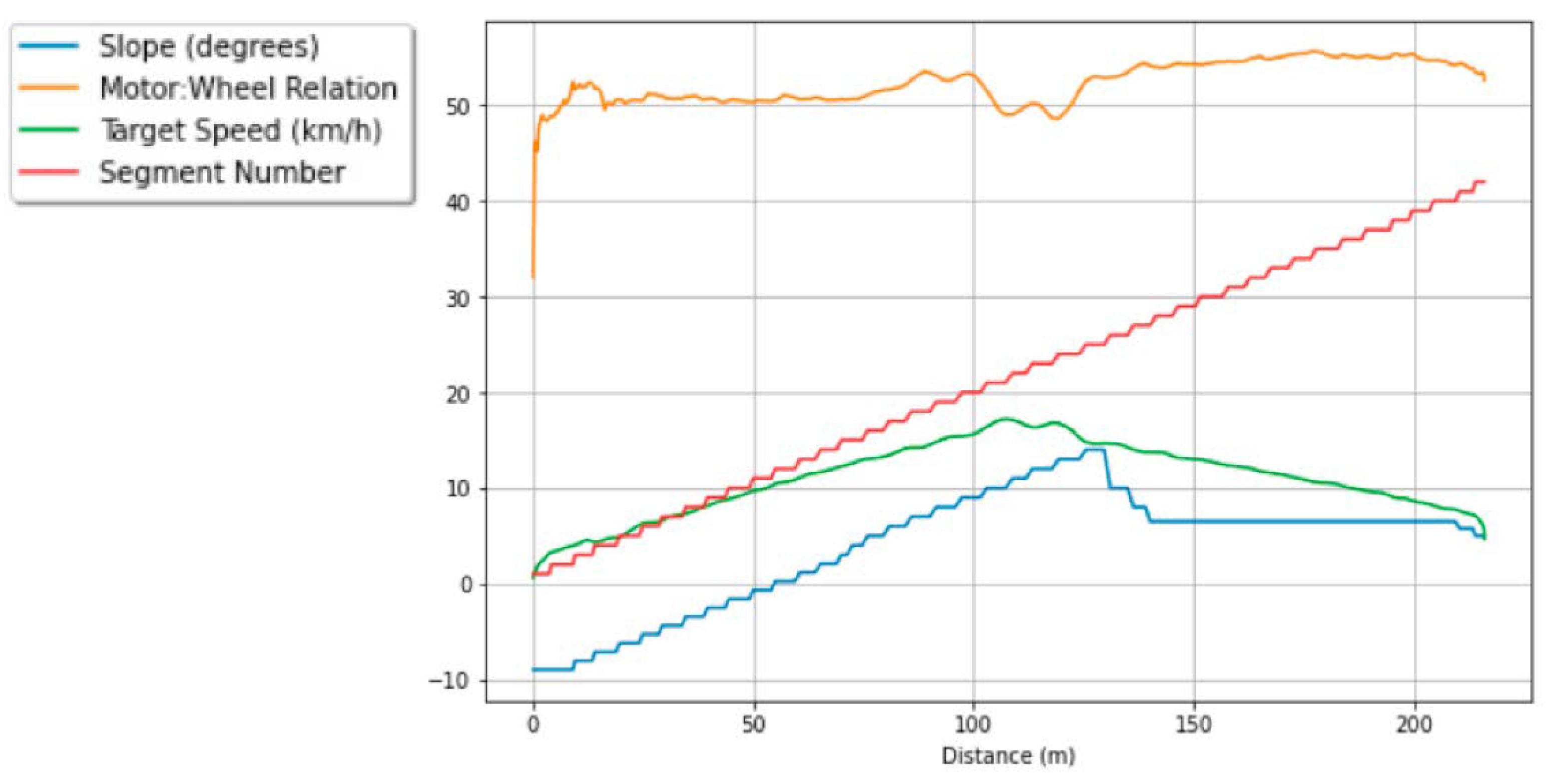
3.1. General Route Information and Data Overview

Figure 10 shows the RPMs and torques measured by both torque meters, the one before and one after the main transmission, as shown in Figure 10. Measurements obtained from the first torquemeter are henceforth called ‘Torque_motor’ and ‘RPM_motor’; whereas those obtained from the second torquemeter are called ‘RPM torquemeter 2’ and ‘Torque Torquemeter 2’. In addition, there is an encoder located on the dynamometer rollers, from which actual road speeds and distance were calculated; this test shows a vehicle accelerating up to a speed of 17.21 km/h and decelerating to 1 km/h. The segment begins with a negative slope starting at −9 degrees, becoming flat in iteration 90, and increasing until iteration 165, with a maximum value of 14 degrees uphill. The point of maximum speed coincides with the point of maximum gradient located at iteration 145. The dynamometer brakes start to apply torque when the sum of torques (‘Torque Sum At Wheel’), as obtained from Equation (4), represented by the cyan line in Figure 10b surpasses zero; however, torques lower than 100 Nm in the wheel were not correctly applied. Inertia torque reaches a maximum value of 198 Nm in iteration 162; while the slope torque has a maximum value of 970 Nm in this same iteration.

From the torque and RPM values measured, power usage as show in Figure 11 is obtained. In it, solid lines (red, yellow, and gray colors) represent the electrical consumption measured by the current and voltage sensors, for the electrical power; and torque and RPM for torquemeters 1 (motor power) and 2 (mechanical power, which takes into account powertrain efficiencies). The dotted lines show the corrected torque considering the simulated dynamics; where the light blue line shows the real power used by the bus motor and the dark blue line the real power of the bus at the rim, after subtracting mechanical losses. In the downhill sections (beginning of this route) the power of the bus is lower than that measured by the sensors thanks to the descending slope contributing most of the torque required for vehicle acceleration.

In Figure 12 the different energy counters are shown, determined by the dynamics of the bus and the sources of work. On solid lines, dyna energy accounts for total energy consumption in the test, while bus energy accounts for actual bus consumption. The dashed lines show the amount of energy spent by the dynamometer to represent inertia or slopes. Inertia energy and slope energy account for total slope and inertia energy, regardless of the source of the work. Dyna inertia energy and dyna slope energy, in pink and cyan respectively, show the amount of energy used by the motor in order represent both phenomena: this is the total amount of energy subtracted from motor energy in order calculate real bus consumption. The negative energy values in the bus energy counter correspond to energy regenerated by the motor, while the positive values correspond to the energy used by the bus. There is a difference of 9.11% between the total energy used by the dynamometer and the real energy of the represented vehicle; this difference will be further elaborated in Section 4.

In the following figures are shown several sections of the route where the particularities of the proposed methodology are evidenced.

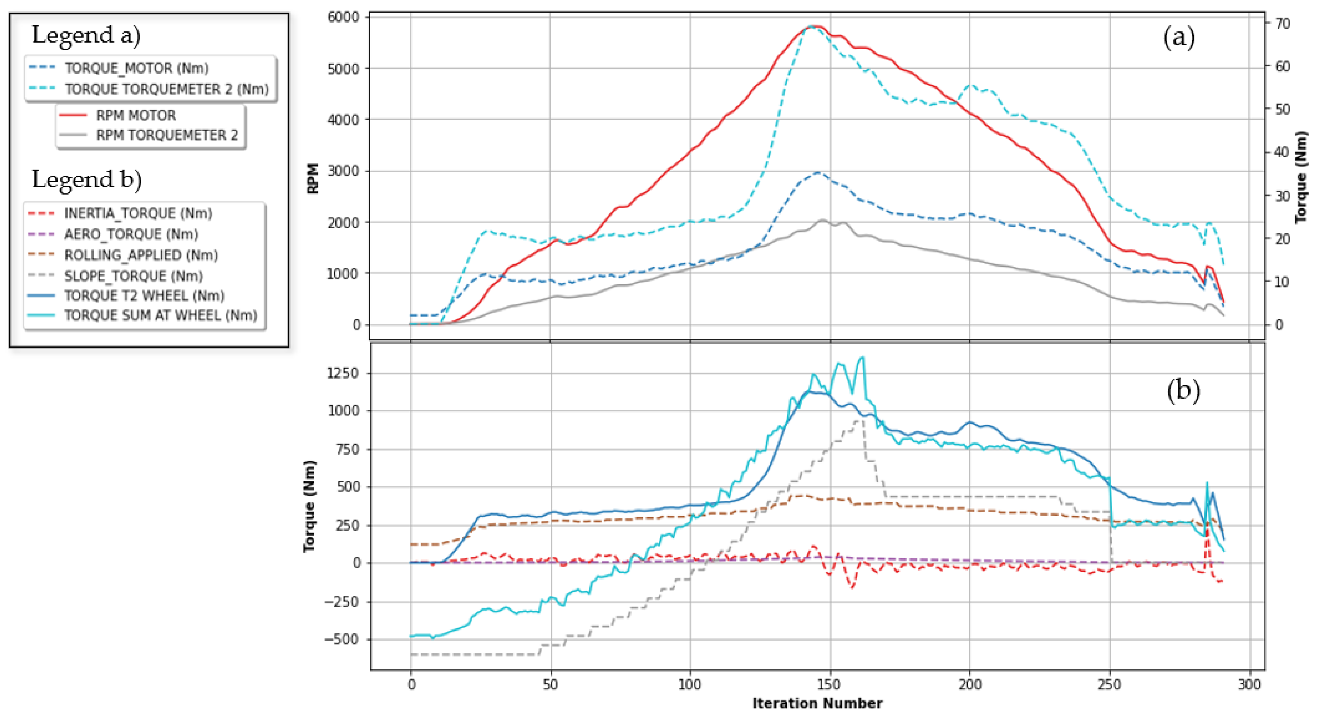
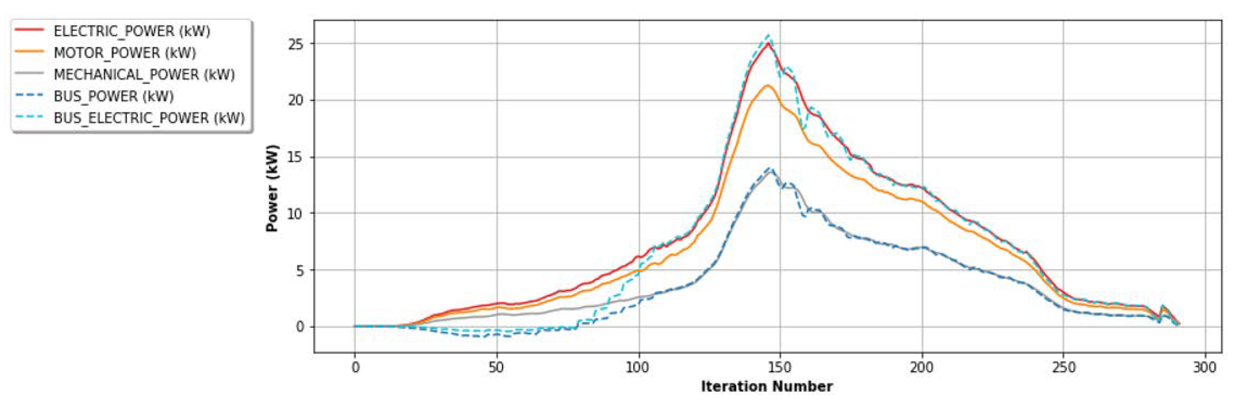
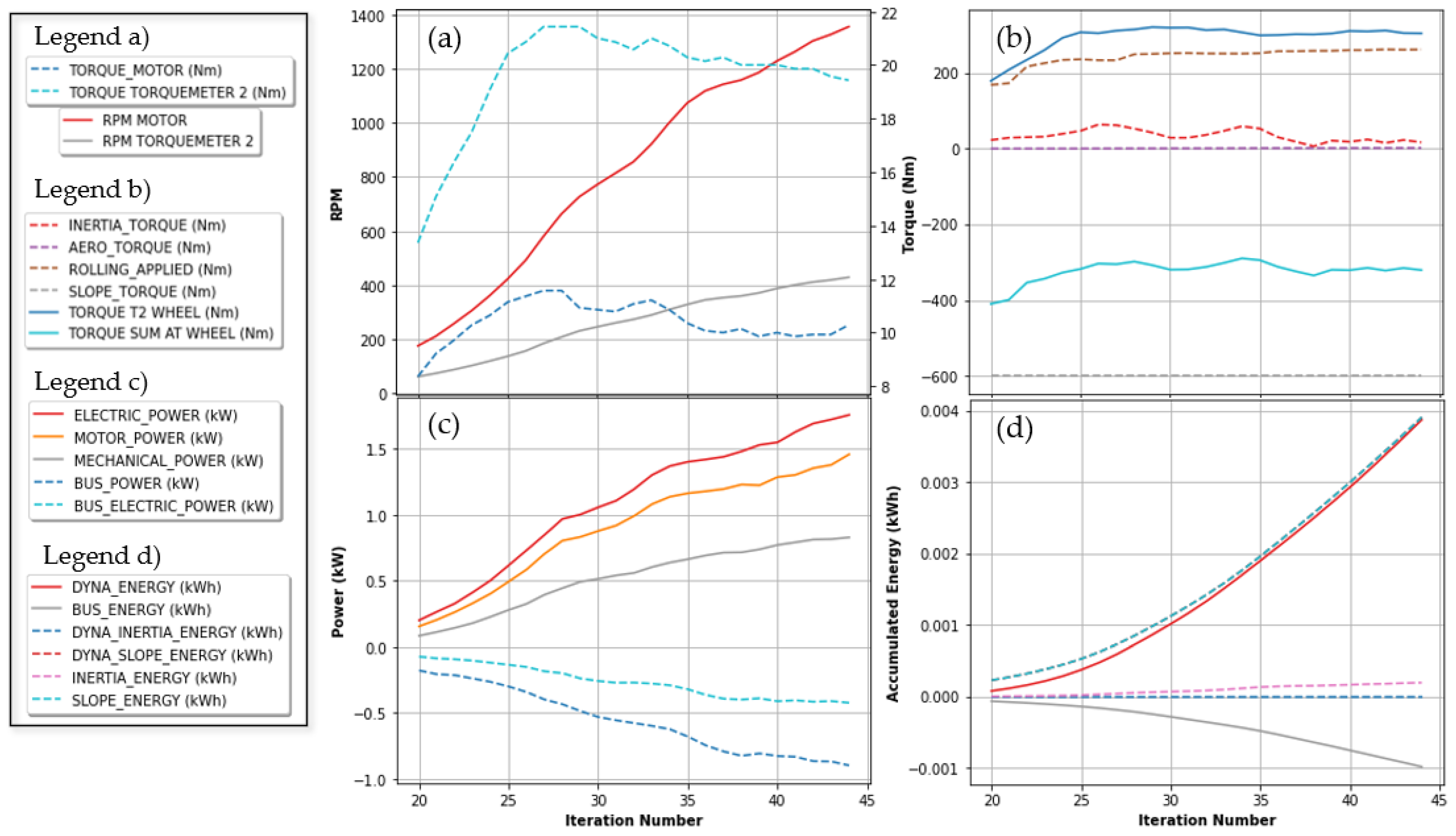
3.2. Analysis of Specific Torque Interactions

The initial half of this route is presented divided in three different sections: (1) a downhill section with a constant slope, (2) a section where the slope changes from downhill to uphill and (3) an uphill section. The three sections presented represent multiple cases of interactions, from those presented in Figure 2, where the vehicle is accelerating: (a) Vehicle accelerating in flat terrain; (d) Vehicle accelerating uphill; (g) Vehicle accelerating downhill. The impact of inertia in deceleration is discussed in Section 4, where the ripple seen from iteration 150 to 170 is commented.

3.2.1. Accelerating Downhill Stretch with Constant Slope

Figure 13 shows a section that starts from rest and in which the bus is on a −9 degree slope. The bus slides slowly downhill while the bus driver brakes and the bus regenerates energy. The slope accelerates the bus overcoming rolling, inertia, and aerodynamic drag. The dotted cyan line in Figure 13c, corresponding to the regenerated electrical power, is lower than the real power in the tire as a function of the losses in the transmission system. Total regeneration for this segment is of 0.0011 kWh; compared to a consumption of 0.0039 kWh by the dynamometer.

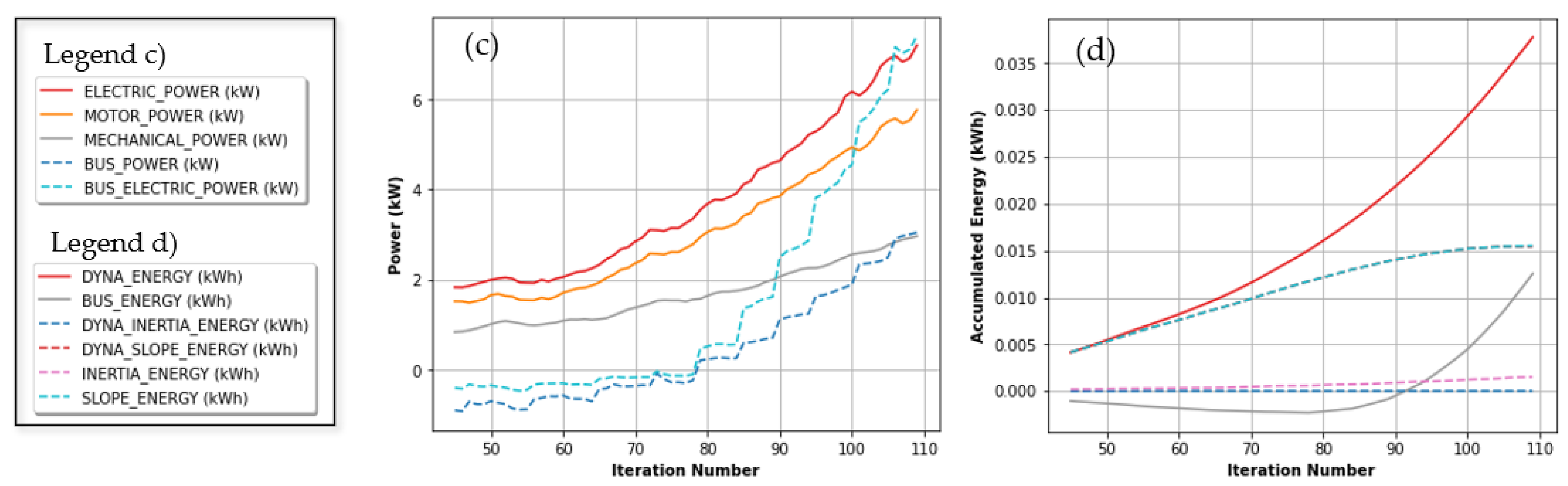
3.2.2. Downhill Section with Changing Slope

Figure 14 shows a section in which the bus accelerates with a slope that changes from −9 degrees to 0 degrees; represented by the torque in Figure 14b. In iteration 78, the slope corresponds exactly to the rolling, negating both effects. Before this iteration the motor does not work to accelerate but to brake, and after this section the motor exerts torque incrementally; this is the reason why in Figure 14c Bus Electric Power is shown to increase as the speed increase continues in the section; with a slope that goes from −9 degrees to 3 degrees. In Figure 14d it can be noticed that at iteration 90 for this route the energy consumed by the bus is 0 kWh, then it increases up to 0.0138 kWh at iteration 110.

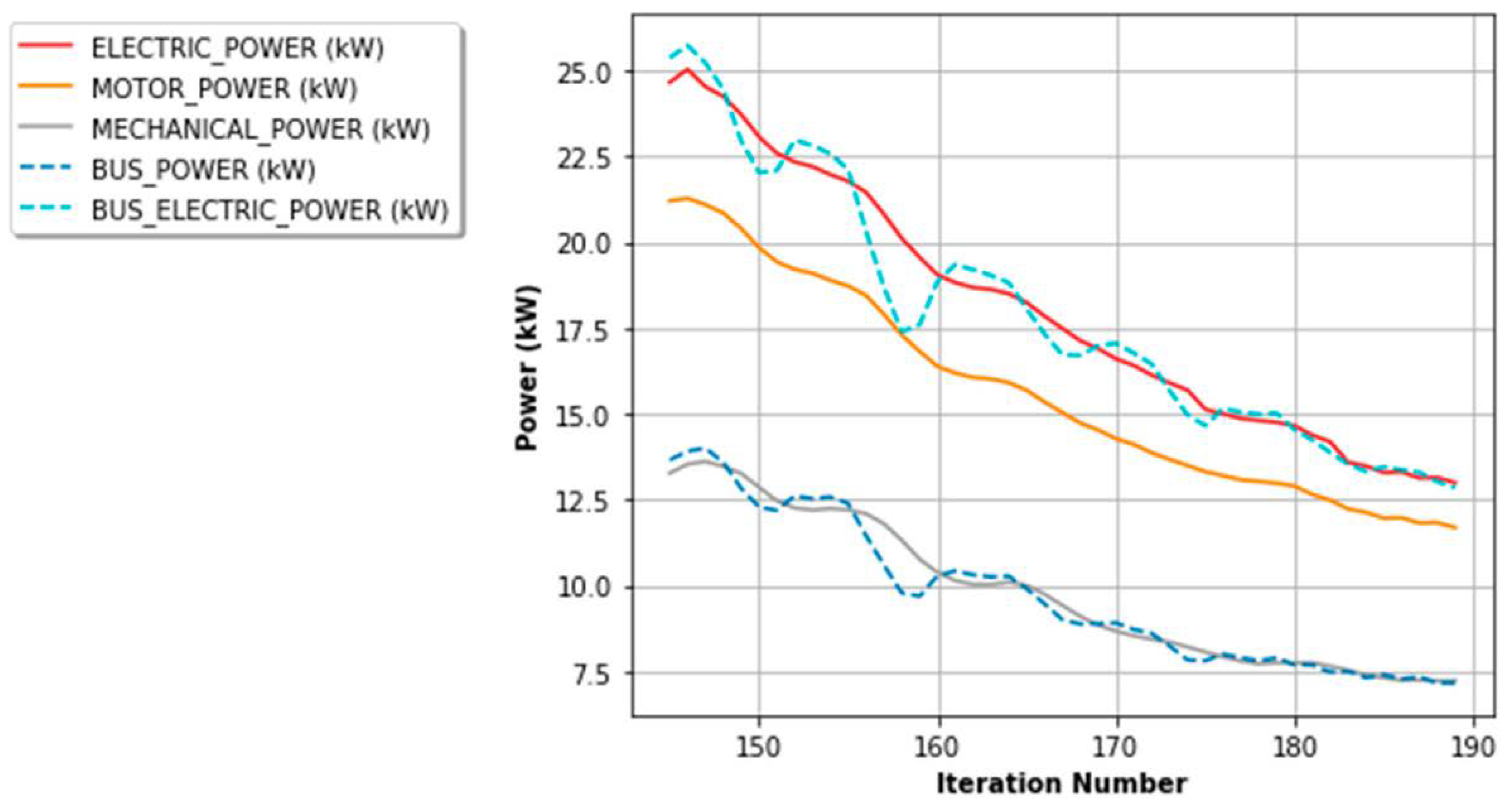
3.2.3. Accelerating Uphill Changing Section

Figure 15 shows a section with torque, power, and consumption values similar to those without using the corrections proposed by this methodology due to the fact that there is a positive slope and an inertia that opposes the movement. Therefore, all torques are opposed to the bus’s movement. For this reason, in Figure 15c, the electrical power and mechanical power lines of the bus correspond directly to those measured by the sensors. From iteration 110 the algorithm tries to apply the difference between the sum of torques and the measured torque, however, there is a lag between the calculated torque to be applied and the measured one; it is also relevant to mention that at iteration 142 that the amount of energy applied by the slope reaches 0; as a function of the energy delivered by the slope in the previous descent and the energy stored by the slope in the last ascent. In this section we can compare the two solid lines of Figure 15b to show that the calculated inertia torque presents a ripple compared to that applied by the brakes of the dynamometer; however, its magnitude never surpasses 30 Nm in this segment, representing less than 3% of the total energy consumption.

4. Discussion

4.1. Inertia Torque Ripple and Iteration Time

Although the method can consider the most relevant driving phenomena through numerical simulation, the time interval between iterations of 0.5 s is a disadvantage in terms of emulation accuracy; however, was necessary in order to ensure proper Modbus communication between the PC and PLCs; as over 100 registers were updated with every read and write command. As mentioned in the results section, the consumption ripple due to changes in speed cannot be emulated (only simulated) with this time-period between iterations due to the brake application time and change in the engine set-point; iteration time proved to be difficult to optimize as brakes and motor have actuation times that differ in multiple orders of magnitude (according to our tests around 100 ms for the motor compared to close to two seconds for the brakes). Because inertia torque is applied after speed changes, braking torque would increase and slow the bus, reducing inertia torque thus allowing for further speed increases resulting in an unstable system, which requires a multi-PID integration within the bus dynamometer transfer function; however, this effect ends up being represented by a smoothed line (as seen in the dotted red line on Figure 15b) that corresponds to the envelope of the torque to be applied; this is largely due to the mechanical damping of the system for sudden accelerations of the motor (depending on the dynamometer’s own inertia and rolling).

Figure 16 shows how despite the ripple caused by inertia simulation, with its limitations mentioned before, actual emulation values properly represent a system with a larger mass, where motor impulse has a lesser effect.

4.2. Energy Calculation Comparison

On the proposed methodology relevant corrections are made in terms of consumption, where for the proposed route a total consumption of 0.302 kWh is obtained, while 0.277 kWh corresponds to the corrected value (9.11% less). The ability to simulate route conditions iteratively, from ground conditions (considered in rolling); to passenger pick-up and drop-off locations or air temperature make this methodology a useful tool for rapid prototyping of powertrains for custom designed vehicles. The regeneration energy of the present method is accurate in terms of the normal operation of the vehicle since it reflects the mechanical and electrical efficiency to carry this energy from the mass of the bus, where it is stored in the form of kinetic and gravitational energy, to the electrical energy entering the battery system.

In a circular route where the bus starts and stops at the same height there is a difference (in our case from 0.0041 kWh to 0.0083 kWh for the inertia) between the energy that the motor delivers to both counters and the energy it can regenerate; this difference is due to non-conservative forces such as bus rolling and efficiency, which in turn depend on the speed of the bus in each segment; however, there are other types of interactions that the method considers; for example, if a vehicle picks up people at the bottom of a slope and drops them at the top, it is possible to emulate the loss of energy corresponding to the work done to raise the passengers. If, on the other hand, the vehicle picks up people at the top and slides down the slope, it could regenerate more energy than it consumed when going uphill.

Table 2. Final energy meters test route.

	Dyna Energy (kWh)	Bus Energy (kWh)	Dyna Inertia Energy (kWh)	Dyna Slope Energy (kWh)	Inertia Energy (kWh)	Slope Energy (kWh)
Mean	0.1344	0.1153	0.0014	0.0122	0.0039	0.0459
Std	0.1190	0.1132	0.0016	0.0054	0.0031	0.0380
Min	0.0000	−0.0023	0.0000	0.0000	0.0000	0.0000
25%	0.0127	0.0000	0.0000	0.0105	0.0006	0.0105
50%	0.1104	0.0872	0.0000	0.0155	0.0038	0.0348
75%	0.2636	0.2392	0.0030	0.0155	0.0071	0.0876
Max	0.3021	0.2769	0.0041	0.0155	0.0083	0.0966

lists the most relevant results in terms of visualizing the bus operation in this section.

Among other remarkable results is the low impact of aerodynamic force on the dynamics of the bus, due to the low speeds of these vehicles on hillside routes. In this route the average value (presented in Table 2) is of 10.78 Nm, corresponding to 2.88% of the torque value used by the bus’s motor to move. On the other hand, the effect of inertia and slope, despite being centered almost at 0 Nm, both in average and in distribution, corresponds to 23.6% and 82.6% of the torque in some sections; it is important to remember that the mass of the selected bus body was 1200 kg, which is between 1/3 and 1/5 part of the real mass of the buses that travel the routes studied in hillside cities. For this reason, the rolling torque, with 39% to 81% of the total torque applied in some sections, has a lower effect proportional to the difference in mass between the simulated vehicle and the real vehicle in operation. Although weight increments affect the rolling its effect is close to one tenth.

Although this method allows for accurate consumption estimation and rapid parameter variation, its main advantage lies in its ability to segment the route into sections according to their energy and power consumption. In this route, 90 of the 250 iterations presented regeneration values, which results in only 0.02 kWh regenerated (due to the low speed of the bus in these sections and its comparatively high rolling); this regeneration corresponds to the actual torque realized by the bus motor to slow down the bus, along with the accompanying efficiencies. A design team for electric bus stops could conclude that the section representing iterations [0, 90] is not a good place to locate charging stations, since the bus would lose the speed accumulated while sliding downhill for a section in which it also has no energy consumption. On the other hand, as can be seen in Table 2, even though for this route there is little regenerated energy, more than 25% (25% percentile of ’bus energy’) of it has no energy consumption; more useful information when spacing the recharging stations. Figure 17 shows the distributions of the total torque and power values.

5. Conclusions

In this paper, a method for accurately representing vehicle dynamics in one motor roller-dynamometers was presented. Through the use of this method, it is possible to accurately and quickly evaluate different routes or vehicles through components or parameters variation. Due to the complex dynamics and the multiplicity of factors, we propose that it is necessary to perform test-runs with the dynamometer in vehicle design; since entirely mathematical models would ignore possible interactions between the vehicle speed changes for the different conditions. Compared to alternatives when using single-motor dynamometers for power consumption tests: (1) simulating only positive slopes does not allow for the correct evaluation of routes in terms of real energy consumption; while (2) measuring consumption only when the motor torque is positive does not consider the possible energy regeneration of the bus, which can be relevant in terms of route planning.

This method is specifically tailored for evaluating bus powertrain configurations in hillside cities which presents route segments with varied topography, where slope and inertia effects are determinant and difficult to evaluate due to the changing vehicle dynamics. Busses on these types of routes are typically rear-wheel drive busses, as forward-wheel drives, despite their high efficiencies are not usually capable of developing enough power in cases where passenger load is located towards the back of the bus, particularly in the steep slopes presented in these cities. Other authors have recently used one motor dynamometers to test Four Wheel Drive vehicles [56] using a similar test route, without taking into account negative inertia and slope values; where the use of this method may help improve their test results. Furthermore, other methods do not include the different $\beta$ parameters mentioned in this article, and thus, conclude that dynamometer tests will always yield similar results for different test runs [57]; this is not the case for this method, however, as the $\beta$ parameters and passengers’ hop-on and off may be modeled through probability distributions, yielding different results for successive runs.

Differences of upwards of 9% in terms of segment energy consumption are observed between the model and traditional one motor dynamometer operation, which become relevant in terms of vehicle or bus route design; these differences are similar to those obtained by Jaworski et al. [58], who evaluated three different types of vehicle load settings (New European Driving Cycle (NEDC), Worldwide Harmonized Light Vehicle Test Procedure (WLTP) and their own calculations) to measure energy consumption on the same vehicle and dynamometer; presenting differences of up to 26%, depending on the load strategy used. Other authors, such as Ligterink et al., have proposed corrections to the WLTP load strategy, obtaining results of up to 10.3% with the original WLTP method. Further research may be of use to compare the proposed method results with those of the established procedures hereby mentioned, as well as other authors’ methods for vehicle representation using chassis dynamometers.

We propose that the accuracy of the model varies as a function of the quality of route information collected, where both road and operating conditions (probability distributions on passenger hop-on and drop-off) are of specific relevance. Although much study has been conducted on simulating vehicle driving in virtual environments, Tsanakas et al.’s approach provide a very thorough test route and kinematic simulation [59], they comment that their model is limited by representing traffic conditions and other parameters aforementioned. Hence, simulations using the numerical methods could use this same mathematical model but would require complementing it with real information on the vehicle operating conditions such as the respective efficiencies of the components for all possible combinations of operation; this research encourages future works to validate the results of this methodology with consumption tests in vehicles, both electric and combustion, on public transportation routes in these types of cities and routes.

References

1. Hanke, C.; Hüelsmann, M.; Fornahl, D. Socio-Economic Aspects of Electric Vehicles: A Literature Review. In Evolutionary Paths Towards the Mobility Patterns of the Future; Springer: Berlin, Germany, 2014; pp. 13–36. [Google Scholar] [CrossRef]
2. Andwari, A.M.; Pesiridis, A.; Rajoo, S.; Martinez-Botas, R.; Esfahanian, V. A review of Battery Electric Vehicle technology and readiness levels. Renew. Sustain. Energy Rev. 2017, 78, 414–430. [Google Scholar] [CrossRef]
3. Wu, Y.; Zhang, L. Can the development of electric vehicles reduce the emission of air pollutants and greenhouse gases in developing countries? Transp. Res. Part D Transp. Environ. 2017, 51, 129–145. [Google Scholar] [CrossRef]
4. Arias-Cazco, D.; Rozas, H.; Jimenez, D.; Orchard, M.E.; Estevez, C. Unifying Criteria for Calculating the Levelized Cost of Driving in Electro-Mobility Applications. World Electr. Veh. J. 2022, 13, 119. [Google Scholar] [CrossRef]
5. Zou, M.; Yang, Y.; Liu, M.; Wang, W.; Jia, H.; Peng, X.; Su, S.; Liu, D. Optimization Model of Electric Vehicles Charging and Discharging Strategy Considering the Safe Operation of Distribution Network. World Electr. Veh. J. 2022, 13, 117. [Google Scholar] [CrossRef]
6. Wang, X.; González, J.A. Assessing Feasibility of Electric Buses in Small and Medium-Sized Communities. Int. J. Sustain. Transp. 2013, 7, 431–448. [Google Scholar] [CrossRef]
7. Vita, V.; Koumides, P. Electric Vehicles and Distribution Networks: Analysis on Vehicle to Grid and Renewable Energy Sources Integration. In 2019 11th Electrical Engineering Faculty Conference (BulEF); IEEE: Varna, Bulgaria, 2019; pp. 1–4. [Google Scholar] [CrossRef]
8. Energy-Efficient Trams and Trolley Buses|CIVITAS. Available online: https://civitas.eu/measure/energy-efficient-trams-and-trolley-buses (accessed on 26 July 2022).
9. Kim, J.; Song, I.; Choi, W. An Electric Bus with a Battery Exchange System. Energies 2015, 8, 6806–6819. [Google Scholar] [CrossRef]
10. Paramesh, K.; Neriya, R.; Kumar, M. Wireless Charging System for Electric Vehicles. Int. J. Veh. Struct. Syst. 2017, 9. [Google Scholar] [CrossRef]
11. Bentalhik, I.; Lassioui, A.; EL Fadil, H.; Bouanou, T.; Rachid, A.; EL Idrissi, Z.; Hamed, A.M. Analysis, Design and Realization of a Wireless Power Transfer Charger for Electric Vehicles: Theoretical Approach and Experimental Results. World Electr. Veh. J. 2022, 13, 121. [Google Scholar] [CrossRef]
12. Nodari, C.; Crispino, M.; Toraldo, E. From Traditional to Electrified Urban Road Networks: The Integration of Fuzzy Analytic Hierarchy Process and GIS as a Tool to Define a Feasibility Index—An Italian Case Study. World Electr. Veh. J. 2022, 13, 116. [Google Scholar] [CrossRef]
13. Tram Systems ‘Too Costly and Underused’|Communities|The Guardian. Available online: https://www.theguardian.com/society/2004/apr/23/communities.politics (accessed on 26 July 2022).
14. Gill, J.S.; Bhavsar, P.; Chowdhury, M.; Johnson, J.; Taiber, J.; Fries, R. Infrastructure Cost Issues Related to Inductively Coupled Power Transfer for Electric Vehicles. Procedia Comput. Sci. 2014, 32, 545–552. [Google Scholar] [CrossRef]
15. How Is This A Good Idea?: EV Battery Swapping—IEEE Spectrum. Available online: https://spectrum.ieee.org/ev-battery-swapping-how-is-this-a-good-idea#toggle-gdpr (accessed on 26 July 2022).
16. Gao, Z.; Lin, Z.; LaClair, T.J.; Liu, C.; Li, J.-M.; Birky, A.; Ward, J. Battery capacity and recharging needs for electric buses in city transit service. Energy 2017, 122, 588–600. [Google Scholar] [CrossRef]
17. Lajunen, A. Energy consumption and cost-benefit analysis of hybrid and electric city buses. Transp. Res. Part C: Emerg. Technol. 2014, 38, 1–15. [Google Scholar] [CrossRef]
18. Peng, K.; Wei, Z.; Chen, J.; Li, H. Hierarchical virtual inertia control of DC distribution system for plug-and-play electric vehicle integration. Int. J. Electr. Power Energy Syst. 2021, 128, 106769. [Google Scholar] [CrossRef]
19. El-Taweel, N.A.; Zidan, A.; Farag, H.E.Z. Novel Electric Bus Energy Consumption Model Based on Probabilistic Synthetic Speed Profile Integrated With HVAC. IEEE Trans. Intell. Transp. Syst. 2021, 22, 1517–1531. [Google Scholar] [CrossRef]
20. Yi, Z.; Bauer, P.H. Adaptive Multiresolution Energy Consumption Prediction for Electric Vehicles. IEEE Trans. Veh. Technol. 2017, 66, 10515–10525. [Google Scholar] [CrossRef]
21. Pelkmans, L.; De Keukeleere, D.; Bruneel, H.; Lenaers, G. Influence of Vehicle Test Cycle Characteristics on Fuel Consumption and Emissions of City Buses. SAE Tech. Rap. 2001, 110, 1388–1398. [Google Scholar] [CrossRef]
22. Adhi, R.P. Top-Down and Bottom-Up Method on Measuring CO2 Emission from Road-Based Transportation System (Case Study: Entire Gasoline Consumption, Bus Rapid Transit, and Highway in Metode Top-Down dan Bottom-Up Dalam Pengukuran Emisi CO 2 dari Sistem Transporta. J. Teknol. Lingkung. 2018, 19, 249–258. [Google Scholar] [CrossRef]
23. Hu, X.; Murgovski, N.; Johannesson, L.; Egardt, B. Energy efficiency analysis of a series plug-in hybrid electric bus with different energy management strategies and battery sizes. Appl. Energy 2013, 111, 1001–1009. [Google Scholar] [CrossRef]
24. Kivekäs, K.; Lajunen, A.; Vepsäläinen, J.; Tammi, K. City Bus Powertrain Comparison: Driving Cycle Variation and Passenger Load Sensitivity Analysis. Energies 2018, 11, 1755. [Google Scholar] [CrossRef]
25. Perger, T.; Auer, H. Energy efficient route planning for electric vehicles with special consideration of the topography and battery lifetime. Energy Effic. 2020, 13, 1705–1726. [Google Scholar] [CrossRef]
26. Zhang, C. Predictive Energy Management in Connected Vehicles: Utilizing Route Information Preview for Energy Saving. 2010. Available online: https://tigerprints.clemson.edu/all_dissertations/649/ (accessed on 26 July 2022).
27. Ruan, J.; Walker, P.; Zhang, N. A comparative study energy consumption and costs of battery electric vehicle transmissions. Appl. Energy 2016, 165, 119–134. [Google Scholar] [CrossRef]
28. Merkisz, J.; Pielecha, J. Emissions and fuel consumption during road test from diesel and hybrid buses under real road conditions. In Proceedings of the 2010 IEEE Vehicle Power Propuls. Conference VPPC 2010, Lille, France, 1–3 September 2010; pp. 2–6. [Google Scholar] [CrossRef]
29. Tica, S.; Živanović, P.; Bajčetić, S.; Milovanović, B.; Nađ, A. Study of the fuel efficiency and ecological aspects of CNG buses in urban public transport in Belgrade. J. Appl. Eng. Sci. 2019, 17, 65–73. [Google Scholar] [CrossRef]
30. Keramydas, C.; Papadopoulos, G.; Ntziachristos, L.; Lo, T.-S.; Ng, K.-L.; Wong, H.-L.A.; Wong, C.K.-L. Real-World Measurement of Hybrid Buses’ Fuel Consumption and Pollutant Emissions in a Metropolitan Urban Road Network. Energies 2018, 11, 2569. [Google Scholar] [CrossRef]
31. Al-Saadi, M.; Mathes, M.; Käsgen, J.; Robert, K.; Mayrock, M.; Van Mierlo, J.; Berecibar, M. Optimization and Analysis of Electric Vehicle Operation with Fast-Charging Technologies. World Electr. Veh. J. 2022, 13, 20. [Google Scholar] [CrossRef]
32. Wang, A.; Ge, Y.; Tan, J.; Fu, M.; Shah, A.N.; Ding, Y.; Zhao, H.; Liang, B. On-road pollutant emission and fuel consumption characteristics of buses in Beijing. J. Environ. Sci. 2011, 23, 419–426. [Google Scholar] [CrossRef]
33. Beckers, C.J.J.; Besselink, I.J.M.; Frints, J.J.M.; Nijmeijer, H. Energy Consumption Prediction for Electric City Buses Citation for Published Version (APA): Energy Consumption Prediction for Electric City Buses. 2019. Available online: https://pure.tue.nl/ws/portalfiles/portal/205351828/20220628_Beckers_hf.pdf (accessed on 26 July 2022).
34. Soltic, P.; Guzzella, L. Optimum SI Engine Based Powertrain Systems for Lightweight Passenger Cars. In SAE Technical Papers; SAE International: Warrendale, PA, USA, 2000. [Google Scholar] [CrossRef]
35. Carlson, R.B.; Wishart, J.; Stutenberg, K. On-Road and Dynamometer Evaluation of Vehicle Auxiliary Loads. SAE Int. J. Fuels Lubr. 2016, 9, 260–268. [Google Scholar] [CrossRef]
36. Singh, N. Fuel Economy Variability Investigations: From Test Cells to Real World. In SAE Technical Papers; SAE International: Warrendale, PA, USA, 2017. [Google Scholar] [CrossRef]
37. Szumska, E.; Jurecki, R.; Pawełczyk, M. Evaluation of the use of hybrid electric powertrain system in urban traffic conditions. Eksploat. i Niezawodn. 2020, 22, 154–160. [Google Scholar] [CrossRef]
38. Mayyas, A.; Prucka, R.; Pisu, P.; Haque, I. Chassis Dynamometer as a Development Platform for Vehicle Hardware In-the-Loop “VHiL”. SAE Int. J. Commer. Veh. 2013, 6, 257–267. [Google Scholar] [CrossRef]
39. William, C., Jr.; Dmitry, S. Dynamometer for Simulating the Inertial and Road Load Forces Encountered by Motor Vehicles and Method. US5445013. 1995. Available online: https://patents.google.com/patent/US5445013A/en (accessed on 23 June 2022).
40. Zhang, X.; Zhou, Z. Research on Development of Vehicle Chassis Dynamometer. J. Phys. Conf. Ser. 2020, 1626. [Google Scholar] [CrossRef]
41. Lohse-Busch, H.; Duoba, M.; Rask, E.; Stutenberg, K.; Gowri, V.; Slezak, L.; Anderson, D. Ambient temperature (20 °F, 72 °F and 95 °F) impact on fuel and energy consumption for several conventional vehicles, hybrid and plug-in hybrid electric vehicles and battery electric vehicle. SAE Tech. Pap. 2013, 2. [Google Scholar] [CrossRef]
42. Kongjian, Q.; Minggao, O.; Qingchun, L.; Maodong, F.; Jidong, G.; Junhua, G. Development and validation of emissions and fuel economy test procedures for heavy duty hybrid electric vehicle. In Proceedings of the 2010 IEEE Vehicle Power and Propulsion Conference, Lille, France, 1–3 September 2010; pp. 1–5. [Google Scholar] [CrossRef]
43. Mayyas, A.R.O.; Kumar, S.; Pisu, P.; Rios, J.; Jethani, P. Model-based design validation for advanced energy management strategies for electrified hybrid power trains using innovative vehicle hardware in the loop (VHIL) approach. Appl. Energy 2017, 204, 287–302. [Google Scholar] [CrossRef]
44. Zha, H.; Zong, Z. Emulating electric vehicle’s mechanical inertia using an electric dynamometer. In Proceedings of the 2010 International Conference on Measuring Technology and Mechatronics Automation, ICMTMA 2010, Changsha, China, 13–14 March 2010; Volume 2, pp. 100–103. [Google Scholar] [CrossRef]
45. Thompson, J.K.; Marks, A.; Rhode, D. Inertia simulation in brake dynamometer testing. SAE Techn. Pap. 2002, 10, 2601. [Google Scholar] [CrossRef]
46. Butler, K.; Ehsani, M.; Kamath, P. A Matlab-based modeling and simulation package for electric and hybrid electric vehicle design. IEEE Trans. Veh. Technol. 1999, 48, 1770–1778. [Google Scholar] [CrossRef] [Green Version]
47. Husain, I.; Islam, M.S. Design, Modeling and Simulation of an Electric Vehicle System. SAE Techn. Pap. 1999, 10, 1149. [Google Scholar] [CrossRef]
48. Malkin, P.; Bisagni, C.; Golinska, P.; Schmitt, D.; Salvato, F. STRIA roadmap on ‘Vehicle Design & Manufacturing’. 2016. Available online: https://trimis.ec.europa.eu/sites/default/files/2021-04/stria_roadmap_-_vehicle_design_and_manufacturing.pdf (accessed on 23 June 2022).
49. Miller, T.; Rizzoni, G.; Li, Q. Simulation-Based Hybrid-Electric Vehicle Design Search. SAE Techn. Pap. 1999, 10, 1150. [Google Scholar] [CrossRef]
50. Bhatt, A. Planning and Application of Electric Vehicle with MATLAB®/simulink®. In Proceedings of the IEEE International Conference on Power Electronics, Drives and Energy Systems, PEDES 2016, Melaka, Malaysia, 28–29 November 2016; Volume 2016-Janua, pp. 1–6. [Google Scholar] [CrossRef]
51. Pathak, A.; Scheuermann, S.; Ongel, A.; Lienkamp, M. Conceptual Design Optimization of Autonomous Electric Buses in Public Transportation. World Electr. Veh. J. 2021, 12, 30. [Google Scholar] [CrossRef]
52. Bottiglione, F.; de Pinto, S.; Mantriota, G.; Sorniotti, A. Energy Consumption of a Battery Electric Vehicle with Infinitely Variable Transmission. Energies 2014, 7, 8317–8337. [Google Scholar] [CrossRef]
53. Xu, Y.; Zheng, Y.; Yang, Y. On the movement simulations of electric vehicles: A behavioral model-based approach. Appl. Energy 2021, 283, 116356. [Google Scholar] [CrossRef]
54. Fiori, C.; Ahn, K.; Rakha, H.A. Power-based electric vehicle energy consumption model: Model development and validation. Appl. Energy 2016, 168, 257–268. [Google Scholar] [CrossRef]
55. Göhlich, D.; Fay, T.-A.; Jefferies, D.; Lauth, E.; Kunith, A.; Zhang, X. Design of urban electric bus systems. Des. Sci. 2018, 4. [Google Scholar] [CrossRef]
56. Shimizu, K.-I.; Nihei, M.; Okamoto, T. Fuel Consumption Test Method for 4WD HEVs – On a Necessity of Double Axis Chassis Dynamometer Test. World Electr. Veh. J. 2008, 2, 253–263. [Google Scholar] [CrossRef]
57. Yang, Z.; Deng, B.; Deng, M.; Huang, S. An Overview of Chassis Dynamometer in the Testing of Vehicle Emission. MATEC Web Conf. 2018, 175, 02015. [Google Scholar] [CrossRef]
58. Jaworski, A.; Mądziel, M.; Lew, K.; Campisi, T.; Woś, P.; Kuszewski, H.; Wojewoda, P.; Ustrzycki, A.; Balawender, K.; Jakubowski, M. Evaluation of the Effect of Chassis Dynamometer Load Setting on CO2 Emissions and Energy Demand of a Full Hybrid Vehicle. Energies 2021, 15, 122. [Google Scholar] [CrossRef]
59. Tsanakas, N.; Ekström, J.; Olstam, J. Generating virtual vehicle trajectories for the estimation of emissions and fuel consumption. Transp. Res. Part C Emerg. Technol. 2022, 138, 103615. [Google Scholar] [CrossRef]
Figure 1. Vehicle accelerating uphill.
Wevj 13 00164 g001
Figure 2. (a) Vehicle accelerating in flat terrain; (b) Vehicle decelerating in flat terrain; (c) Vehicle in constant speed in flat terrain; (d) Vehicle accelerating uphill; (e) Vehicle decelerating uphill; (f) Vehicle in constant speed uphill; (g) Vehicle accelerating downhill; (h) Vehicle decelerating downhill; (i) Vehicle in constant speed downhill.
Wevj 13 00164 g002
Figure 3. Efficiency Map for an electric motor.
Wevj 13 00164 g003
Figure 4. Mirrored efficiency map for regenerative torque.
Wevj 13 00164 g004
Figure 5. Energy and information flows in the dynamometer.
Wevj 13 00164 g005
Figure 6. Route plot for an entire bus route on a hillside city.
Wevj 13 00164 g006
Figure 7. General Operation Algorithm.
Wevj 13 00164 g007
Figure 8. Dynamometer used for model evaluation.
Wevj 13 00164 g008
Figure 9. Test route data.
Wevj 13 00164 g009
Figure 10. (a) Measured torque and RPM; (b) applied torques.
Wevj 13 00164 g010
Figure 11. Calculated and corrected powers integer route.
Wevj 13 00164 g011
Figure 12. Calculated and measured energies entire route.
Wevj 13 00164 g012
Figure 13. Accelerating downhill stretch with constant slope. (a) Torques and RPMs measured by dynamometer sensors. (b) Torques values per origin force. (c) Dynamometer power and equivalent bus power. (d) Accumulated energy for the whole route.
Wevj 13 00164 g013
Figure 14. Downhill section with changing slope. (a) Torques and RPMs measured by dynamometer sensors. (b) Torques values per origin force. (c) Dynamometer power and equivalent bus power. (d) Accumulated energy for the whole route.
Wevj 13 00164 g014aWevj 13 00164 g014b
Figure 15. Accelerating uphill changing section. (a) Torques and RPMs measured by dynamometer sensors. (b) Torques values per origin force. (c) Dynamometer power and equivalent bus power. (d) Accumulated energy for the whole route.
Wevj 13 00164 g015
Figure 16. Deceleration section with changing slope.
Wevj 13 00164 g016
Figure 17. (a) Torque boxplot; (b) Power boxplot.
Wevj 13 00164 g017