

Research on Short-Term Driver Following Habits Based on GA-BP Neural Network


 , and
, and
Abstract
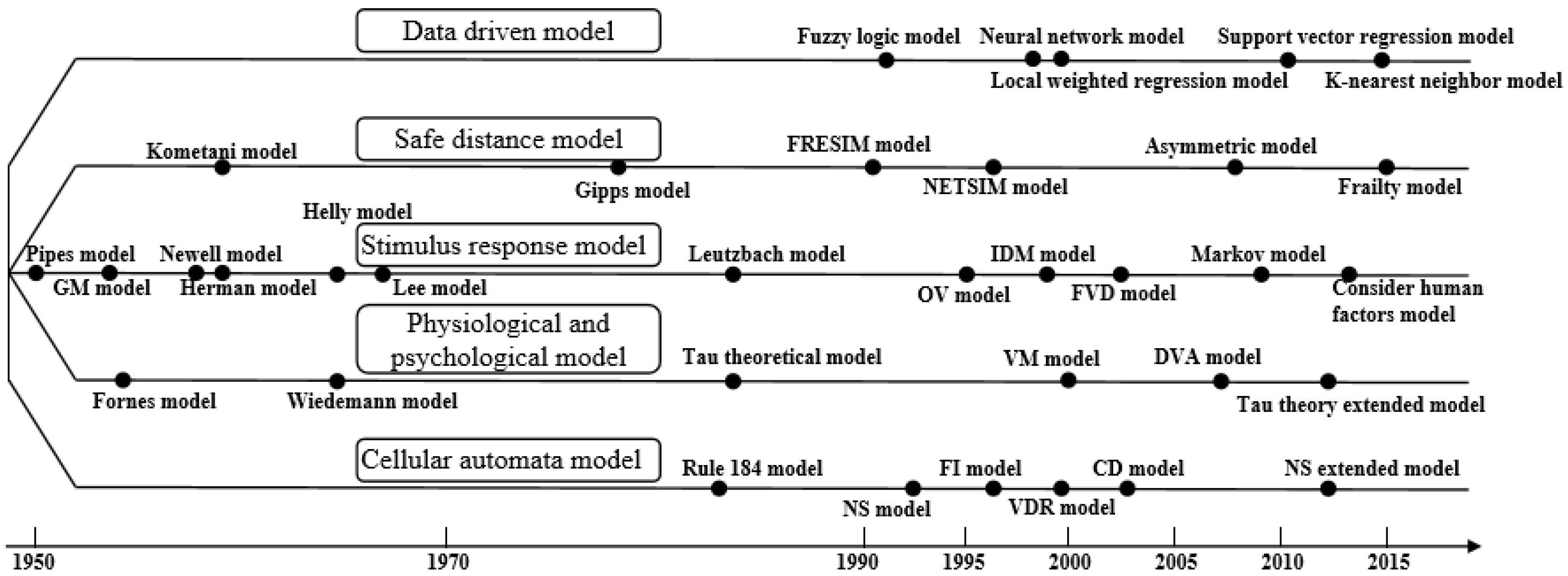
:1. Introduction
2. Data Acquisition and Analysis
Data Sources
3. Adaptive Processing
3.1. Data Preprocessing
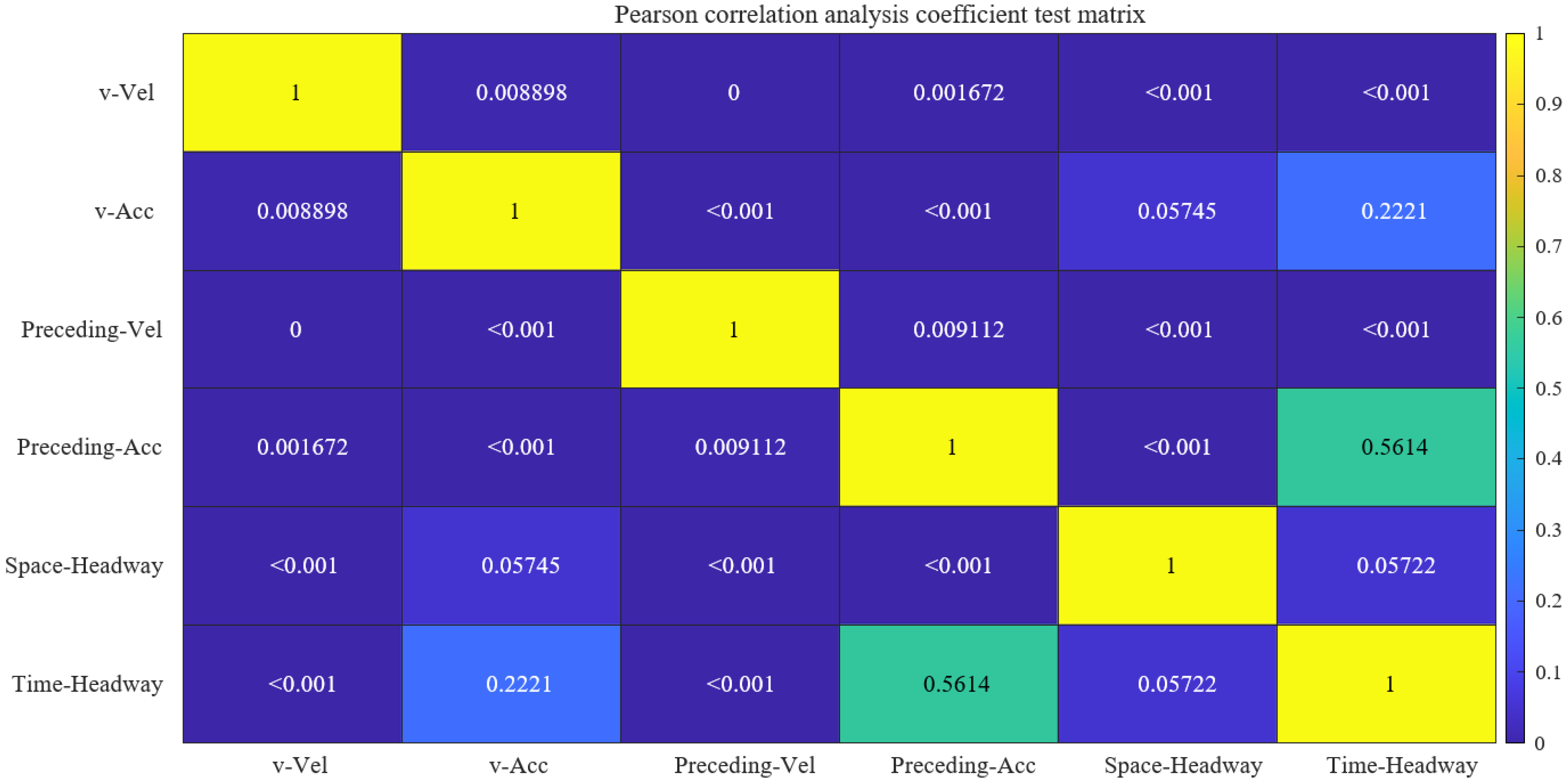
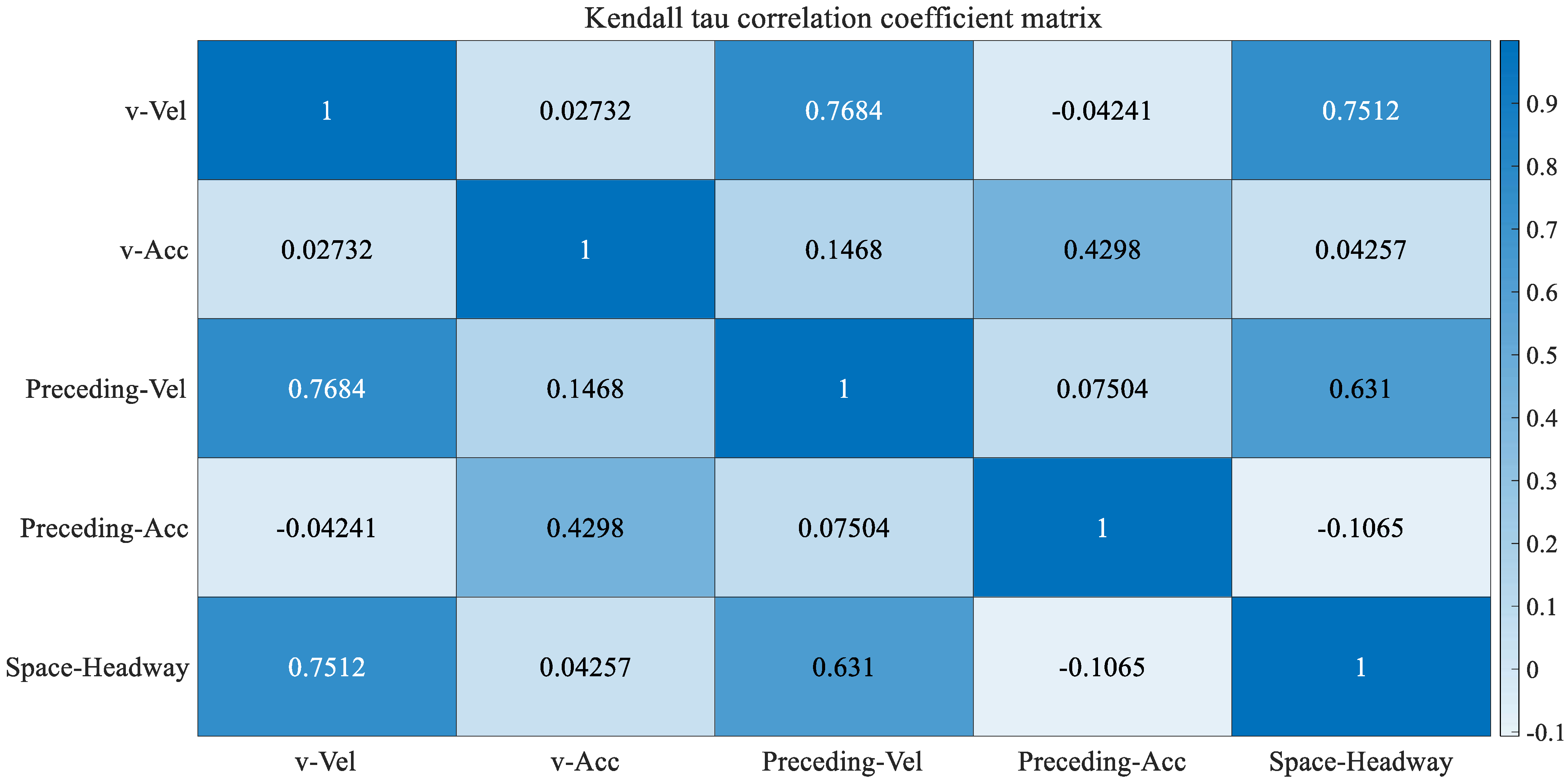
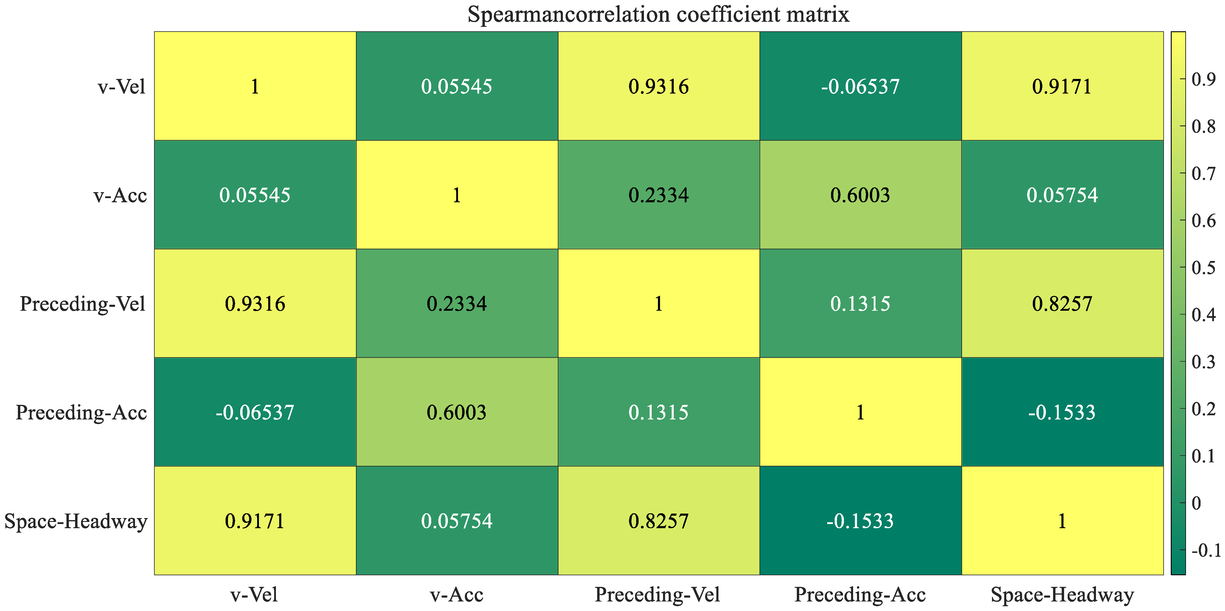
3.2. Correlation Analysis
4. Car-following Model
4.1. Stimulus-Response Model
4.2. Driver Habit Learning Model Based on GA-BP Neural Network
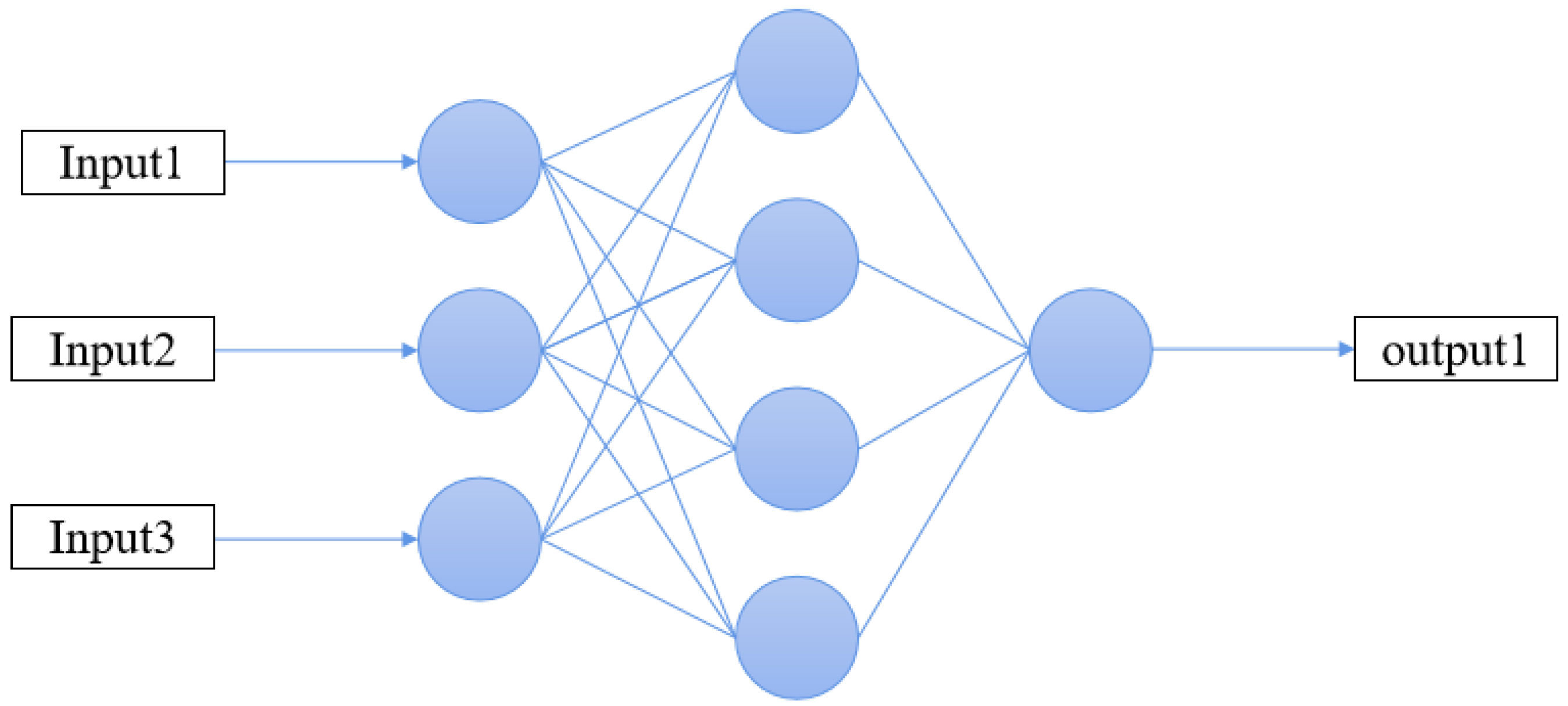
4.2.1. BP Neural Network
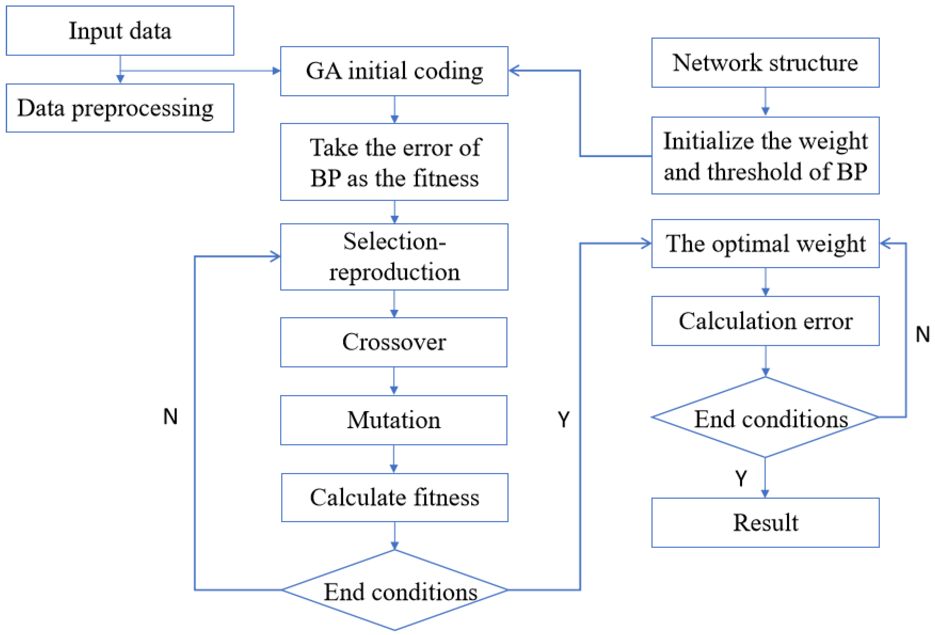
4.2.2. Genetic Algorithm (GA)
- (1)
- Population initialization:
- (2)
- Fitness function:
- (3)
- Selection operation:
- (4)
- Crossover operation:
- (5)
- Variation operation:
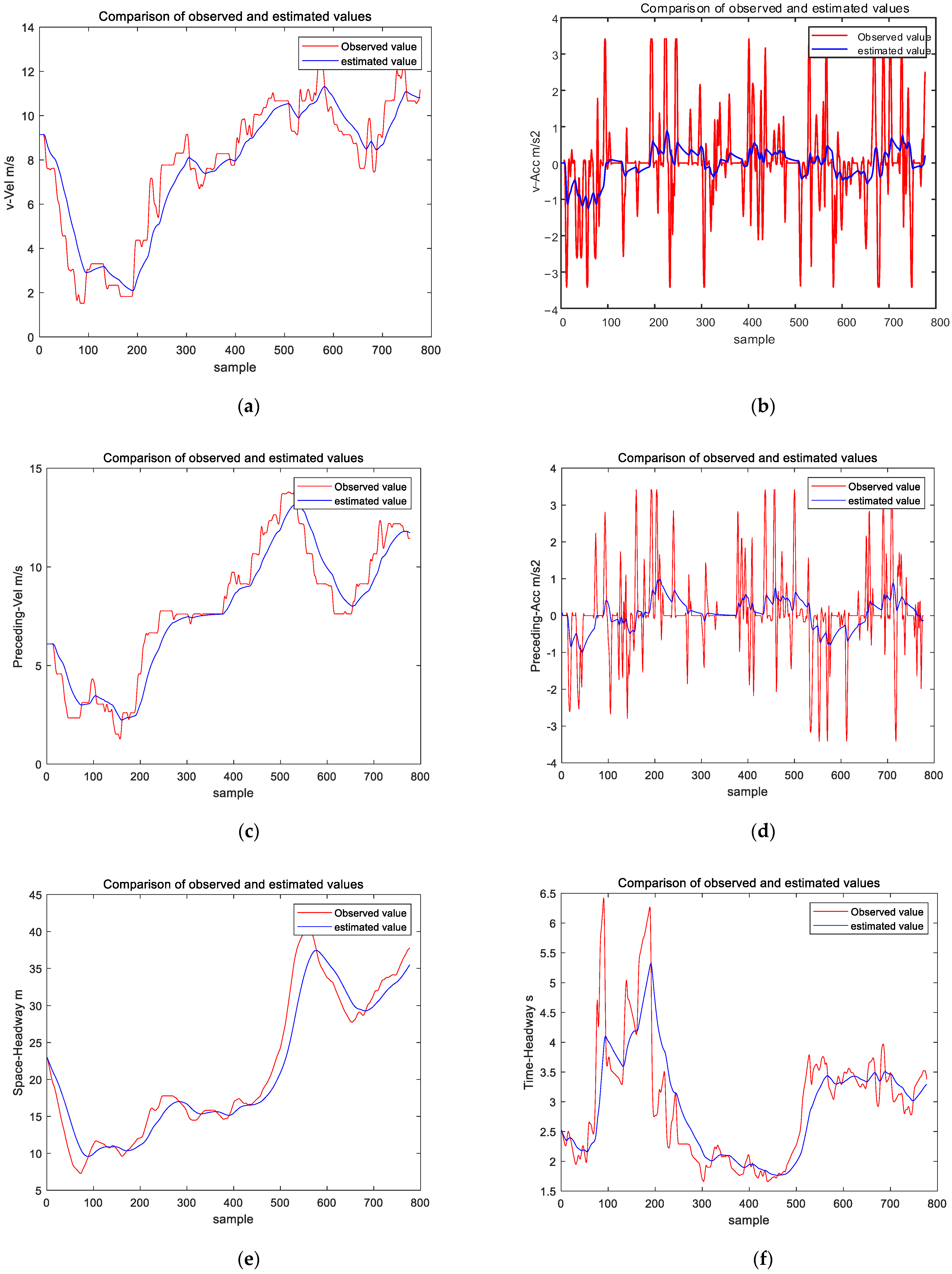
5. Simulation Verification
5.1. Simulation Scenario
- (1)
- Only two vehicles (the preceding vehicle and main vehicle) exist in this scenario;
- (2)
- The driving line is in a straight line (the same as for the ngsim data set);
- (3)
- The driving speed of the preceding vehicle in the simulation process uses the Preceding_Vel data in ngsim;
- (4)
- In the experimental group, the driving strategy of the main vehicle was decided by the trained neural network, while in the control group, the driving strategy of the main vehicle was a stimulus-response model;
- (5)
- An instantaneous change in vehicle acceleration is allowed, but speed is not allowed.
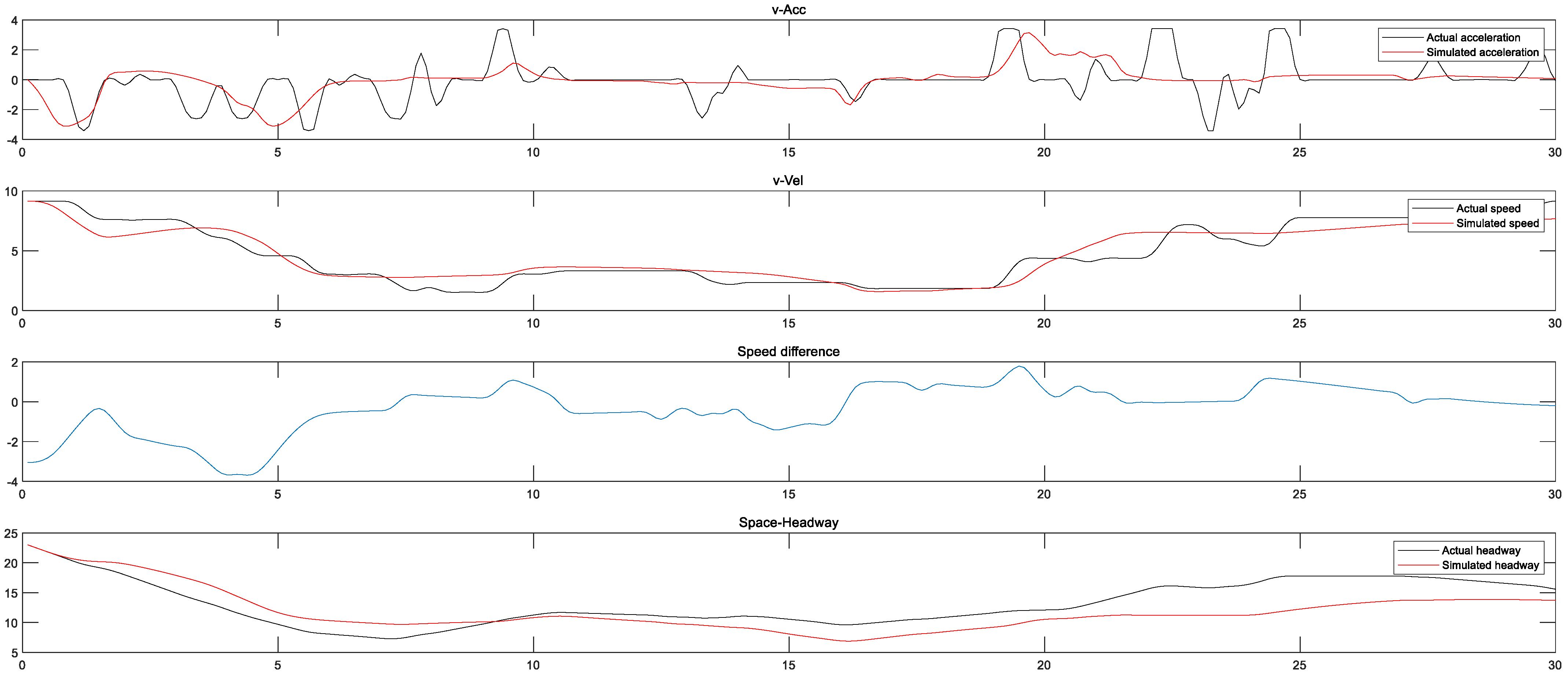
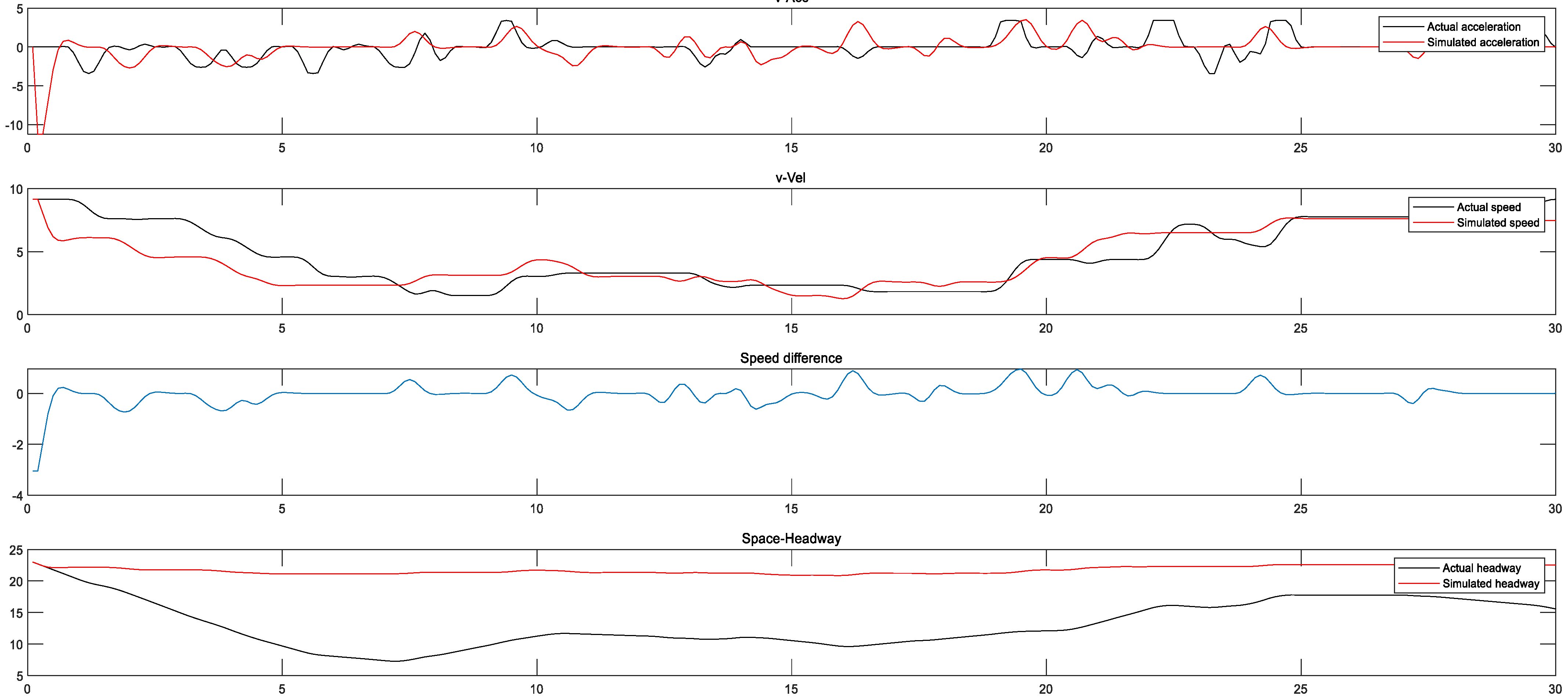
5.2. Car-following Simulation
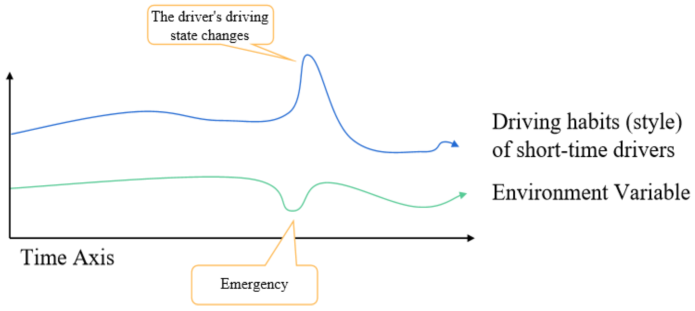
5.2.1. Explaining This Assumption
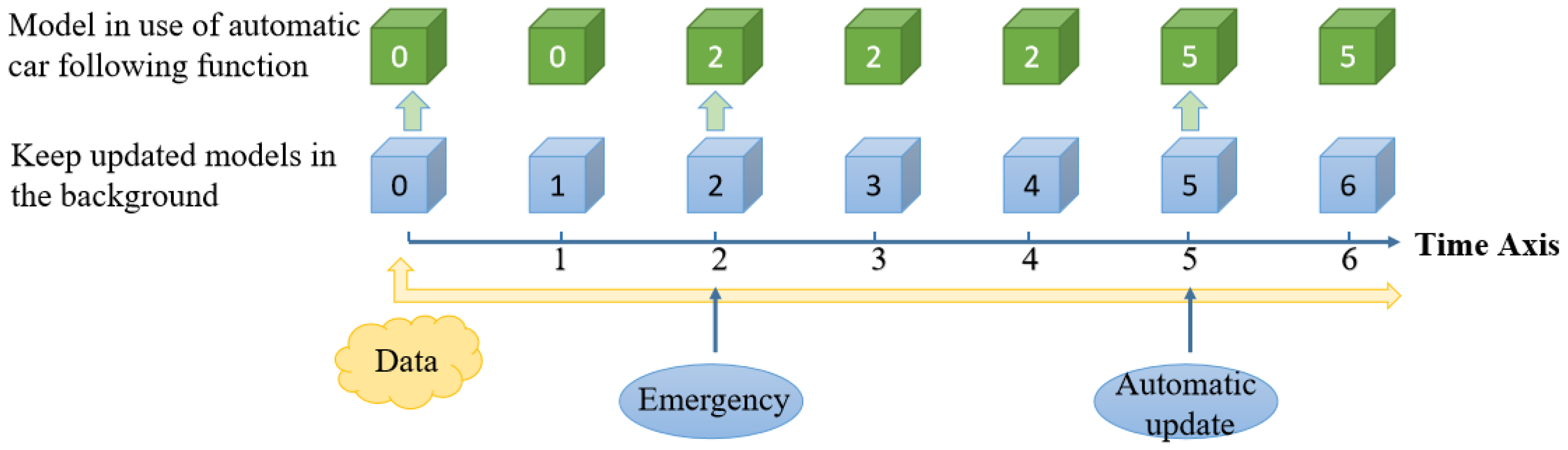
5.2.2. Application Scheme
- (1)
- To maintain data collection during the whole process of the driver driving the vehicle; this data should at least include the five main parameters mentioned in the paper.
- (2)
- Using the latest data collected, the model is constantly updated over time (blue cube in Figure 10).
- (3)
- The model used in the automatic car-following function is the green cube in Figure 10. This model will be updated in the following three cases:
- Automatic update with a cycle of 5 unit times.
- Driver’s active intervention (the automatic car-following function is on).
- When the automatic car-following function is not enabled, the system will also use the model (green cube) to predict the car-following status in real time and compare it with the real status of the vehicle. When the error is greater than the threshold, the model will be updated. (If the vehicle leaves the following state for 5 s, the system stops).
- (4)
- The automatic updating speed of the model is determined by the computing power of the vehicle VCU.
5.3. Car-following Simulation
6. Conclusions
Author Contributions
Funding
Data Availability Statement
Conflicts of Interest
References
- World Health Organization. Global Status Report on Road Safety 2018: Summary; World Health Organization: Geneva, Switzerland, 2018.
- Fagnant, D.J.; Kockelman, K. Preparing a nation for autonomous vehicles: Opportunities, barriers and policy recommendations. Transp. Res. Part A Policy Pract. 2015, 77, 167–181. [Google Scholar] [CrossRef]
- Qiao, W. Research Status and Development of Vehicle Passive Safety. Trans. Chin. Soc. Agric. Mach. 2005, 9, 36. [Google Scholar]
- Editorial Office. Review on China’s Automotive Engineering Research Progress: 2017. China J. Highw. Transp. 2017, 30, 1–197. [Google Scholar] [CrossRef]
- Liang, W.; Hong, F. Overview of ADAS technology and market status. Technol. Innov. 2021, 7, 6–9+13. [Google Scholar] [CrossRef]
- Reuschel, A. Vehicle movements in the column uniformly accelerated or delayed. Oesterreich Ingr. Arch. 1950, 4, 193–215. [Google Scholar]
- Pipes, L.A. An operational analysis of traffic dynamics. J. Appl. Phys. 1953, 24, 274–281. [Google Scholar] [CrossRef]
- Yang, H.; Chun, Z.; Chou, X.; Shuai, L.I.; Wang, H. Research progress on car-following model. J. Traffic Transp. Eng. 2019, 19, 125–138. [Google Scholar] [CrossRef]
- Zhang, S.; Wang, H.; Chen, P.; Zhang, X.; Li, Q. Overview of the application of neural networks in the motion control of unmanned vehicles. Chin. J. Eng. 2022, 44, 235–243. [Google Scholar] [CrossRef]
- Zhong, J.; Yang, S. Review of Fuzzy ARTMAP neural network. Comput. Sci. 2001, 5, 89–92. [Google Scholar]
- Yang, L.; Zhao, S.; Xu, H. Car-following model based on the modified optimal velocity function. J. Transp. Syst. Eng. Inf. Technol. 2017, 17, 41–46. [Google Scholar]
- Bolduc, A.P.; Guo, L.; Jia, Y. Multimodel approach to personalized autonomous adaptive cruise control. IEEE Trans. Intell. Veh. 2019, 4, 321–330. [Google Scholar] [CrossRef]
- Liu, Z.Q.; Zhang, K.D.; Ni, J. Analysis and identification of drivers’ difference in carfollowing condition based on naturalistic driving data. J. Transp. Syst. Eng. Inf. Technol. 2021, 21, 48–55. [Google Scholar]
- Newell, G.F. Memoirs on Highway Traffic Flow Theory in the 1950s. Oper. Res. 2002, 50, 173–178. [Google Scholar] [CrossRef]
- Coifman, B.; Li, L. A critical evaluation of the Next Generation Simulation (NGSIM) vehicle trajectory dataset. Transp. Res. Part B 2017, 105, 362–377. [Google Scholar] [CrossRef]
- Huang, C.; Lin, F. Vehicle States Estimation Algorithm Based on Combination of S-correction Adaptive Kalman Filter and Fuzzy Kalman Filter. China Mech. Eng. 2013, 24, 2831–2835. [Google Scholar]
- Jing, M.; Wang, H.; Wang, W. Heterogeneous car following models based on data analysis. J. Jilin Univ. Sci. Ed. 2015, 45, 761–768. [Google Scholar] [CrossRef]
- Yang, D.; Pu, Y.; Yang, F.; Zhu, L. Car-following model based on optimal distance and its characteristics analysis. J. Southwest Jiaotong Univ. 2012, 47, 888–894. [Google Scholar]
- Yang, H.; Li, H.; Hu, H.; Liu, C.; Rui, L.; Qiao, Y. Multi-Guided Vehicle’s Influence on Car-following Driving Characteristics under Different Speed. Mod. Transp. Technol. 2019, 16, 72–76. [Google Scholar]
- Wang, K.; Yang, Y.; Wang, S.; Shi, Z. Research on Car-Following Model considering Driving Style. Math. Probl. Eng. 2022, 2, 1–9. [Google Scholar] [CrossRef]


| Column Name | Description | Unit |
|---|---|---|
| Vehicle_ID | Vehicle identification number. | - |
| Frame_ID | The number of frames of the data at a certain time. | 0.1 s |
| Total_Frame | The total number of frames of this vehicle in this dataset. | 0.1 s |
| Global Time | Time stamp. | ms |
| Local_X | Abscissa of the center of the front of the vehicle. | Feet |
| Local_Y | Ordinate of the center of the front of the vehicle. | Feet |
| Global_X | Abscissa of the vehicle in the global coordinate system. | Feet |
| Global_Y | Ordinate of the vehicle in the global coordinate system. | Feet |
| v_length | Vehicle length. | Feet |
| v_width | Vehicle width. | Feet |
| v_Class | Vehicle class: 1—Motorcycle; 2—Light-Duty Vehicle; 3—Large Vehicle. | - |
| v_Vel | Instantaneous speed of the vehicle. | Feet/s |
| v_Acc | Instantaneous acceleration of the vehicle. | Feet/s2 |
| Lane_ID | Current lane position of the vehicle. | - |
| Preceding | Vehicle ID of the vehicle in front of the same lane. | - |
| Following | Vehicle ID of the vehicle following the vehicle in the same lane. | - |
| Space_Headway | Distance from the front center of the vehicle to the front center of the front vehicle. | Feet |
| Time_Headway | Time required for two vehicles to pass the same position | s |
Publisher’s Note: MDPI stays neutral with regard to jurisdictional claims in published maps and institutional affiliations. |
© 2022 by the authors. Licensee MDPI, Basel, Switzerland. This article is an open access article distributed under the terms and conditions of the Creative Commons Attribution (CC BY) license (https://creativecommons.org/licenses/by/4.0/).
Share and Cite
Wu, C.; Li, B.; Bei, S.; Zhu, Y.; Tian, J.; Hu, H.; Tang, H. Research on Short-Term Driver Following Habits Based on GA-BP Neural Network. World Electr. Veh. J. 2022, 13, 171. https://doi.org/10.3390/wevj13090171
Wu C, Li B, Bei S, Zhu Y, Tian J, Hu H, Tang H. Research on Short-Term Driver Following Habits Based on GA-BP Neural Network. World Electric Vehicle Journal. 2022; 13(9):171. https://doi.org/10.3390/wevj13090171
Chicago/Turabian StyleWu, Cheng, Bo Li, Shaoyi Bei, Yunhai Zhu, Jing Tian, Hongzhen Hu, and Haoran Tang. 2022. "Research on Short-Term Driver Following Habits Based on GA-BP Neural Network" World Electric Vehicle Journal 13, no. 9: 171. https://doi.org/10.3390/wevj13090171
APA StyleWu, C., Li, B., Bei, S., Zhu, Y., Tian, J., Hu, H., & Tang, H. (2022). Research on Short-Term Driver Following Habits Based on GA-BP Neural Network. World Electric Vehicle Journal, 13(9), 171. https://doi.org/10.3390/wevj13090171