Abstract
Smart transformation and green development are the core research directions of electric vehicles. An electric tractor is powered by the vehicle battery. The motor converts electric energy into mechanical energy and drives the wheels through the drive train. Therefore, the electric tractor model is a modular mathematical model for the battery, motor, drive train, and drive wheel. A class of high-order terminal sliding mode control strategies is adopted to establish the relative rotational angles of drive wheels, driving angular speeds, and motor angular speeds as input, and driving angular speeds and motor angular speeds as output. This process ensures stable operating speed and good working quality under the operating conditions and achieves small-scale unattended driving. The output is a nonlinear system state equation. An n-order derivative continuous function is introduced to design the terminal sliding surface of the sliding mode. A control function to reduce chattering is also designed to ensure that the output function converges at the finite time and the existing sliding stage achieves zero steady-state error. Simulation results of the whole electric tractor model show that the speed remains stable under the condition of outside interference, and experiments verify the feasibility of the control strategy.
1. Introduction
As a green dynamic machine with zero emissions, no pollution, and low noise, the electric tractor will become one of the important contributions to the further development of modern agricultural tractors, and it also represents the development direction of new energy technology in the field of agricultural machinery [1]. The rapid development of new energy technology and the research and development of electric tractors provide a new way for the development of environmental protection and green agricultural machinery products [2], and the development of electric tractors will also help the intelligent integrated construction of precision agriculture [3,4].
An intelligent electric tractor must have a “brain” to control the vehicle’s operation. Given the harsh working environment of electric tractors, sudden load changes, low speed, large torque, and wide speed range [5], numerous signals at different times should be collected and processed to achieve intelligence. In the current industry, PID algorithm [6] is used for the signal processing of motor speed control. PID is mainly used for relatively accurate mathematical models to achieve online adjustment. However, it has many limitations. The PID algorithm of the traditional regulating motor is unsuitable for the vehicle control system of an electric tractor because of the system’s multiple variables. Moreover, the control system of an electric tractor is nonlinear and suffers from random interference.
The main function of the electric controller is to collect the driver’s operation signals and various sensor signals to control the motor speed and meet its own requirements. Few studies on intelligent controllers for electric tractors have been conducted. Moreover, the research mainly focused on the field of power shifting. The “brain” of an electric tractor’s intelligent controller is the core of the entire operation process. However, few studies on the intelligent control of the electric tractor have been conducted. The working condition of the electric tractor is complicated, and the operation quality is poor in the case of plowing and sowing. Therefore, analyzing the stability of speed in the case of external disturbance is necessary. Artificial intelligence (AI) algorithms [7,8,9] have more applications in the control field, and have achieved an important position. Terminal sliding mode control [10] is a type of control strategy for high-order nonlinear systems. In the design of the sliding hyperplane, a nonlinear function is introduced to construct the sliding surface so the tracking error can converge to zero at the finite time [11]. In [12,13], a system with a delayed state is considered and the switching surface of the terminal is designed by fuzzy algorithm. The time delay is a known constant, and the full state vector is available for feedback. Therefore, the adaptive algorithm is used to adjust the sliding mode control of the uncertain time-varying system. In [14,15], one of the simplest and most popular methods to design a model-based controller for a nonlinear dynamic system is to apply linear control theories to the linearized model of the nonlinear system. Different strategies were proposed to increase the robustness of linearization-based control methods against the linearization error. For example, a Hu terminal slip surface for high-order nonlinear systems is designed to overcome the shortcomings of sliding mode discontinuities and ensure robustness and stability. In [16], the average value of a high-frequency switching signal in the adaptive law can be provided by Arie Levant’s differentiator rather than a low-pass filter. The rigorous mathematical proof verifies that the system states can converge to the origin within a finite time under the proposed adaptive nonsingular terminal sliding mode (NTSM) controller. The adaptive terminal controller design of the multi-input and multi-output (MIMO) system is achieved for unknowns and uncertainties of the external system. In [17], a new continuous terminal sliding mode control algorithm is proposed to guarantee that the system states reach the sliding surface in finite-time. Not only is the robustness guaranteed by the proposed controller, but the continuity also makes the control algorithm more suitable for the servo mechanical systems. In [18,19], the sliding mode surface is based on different designs, and a new sliding-mode control for an underactuated flexible joint robot is proposed to guarantee the finite-time convergence of the systems output, and to achieve the total robustness against the lumped disturbance and estimation error. The sliding mode algorithm is fully consistent with the external disturbance and parametric perturbation control of electric tractors during operation. Using the switching surface design and external interference value is reasonable to prevent singular problems. This algorithm not only ensures fast tracking in time but also addresses the chattering problem [20].
Based on the above analysis, a method for electric tractor molding based on a terminal sliding mode control algorithm is proposed in this paper. Firstly, the whole vehicle state model of the electric tractor is established. Secondly, the sliding mode surface and the sliding mode controller to reduce chattering are designed. Finally, the simulation and experimental verification of the whole vehicle model of the electric tractor show that the electric tractor based on the terminal sliding mode control algorithm can be maintained in a stable state, which is stronger than the PID control robustness based on the physical model.
2. State Equation of the Electric Tractor
This study uses the rear wheel two-wheel drive form to analyze the electric tractor. If the electric tractor needs to achieve unmanned operation under a forest or greenhouse, then it must meet the requirements of different sudden load conditions to adjust the motor speed in time and ensure stability and automatic control of the electric tractor’s speed. According to tractor theory and automobile control theory, an electric tractor is mainly composed of an electric motor module, a power supply module, a drive train module, and a drive wheel module. Figure 1 illustrates the structural diagram of an electric tractor, where the reduction gearbox is included in the drive train.
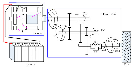
Figure 1.
Diagram of an electric tractor. Note: 1—electronic commutation switch circuit, 2—sensor rotor, 3—main rotor, 4—main stator, and 5—sensor stator.
2.1. Modular Model
2.1.1. Motor Model
For electric tractors working in different environments, the motor should meet the following requirements: low speed, high torque, overload capacity, high resistance, simple structure, and easy maintenance conditions. The brushless DC motor used in the electric tractor has low voltage characteristics, torque overload capacity, start torque, and small start current characteristics. The motor equations [21] are shown in Equations (1)–(6).
The basic motion equation of the motion control system is expressed as follows:
where is the electromagnetic torque (N·m); is the output torque (N·m) of the motor output shaft; is the damping torque coefficient; is the mechanical angular velocity (rad/s) of the rotor of the motor; and J is the mechanical moment of inertia (kg·m2) for the motor output shaft.
The voltage balance equation is expressed as
where U is the rectified voltage (V) at both ends of the motor, E is the armature-winding-induced electromotive force, I is the armature current (A), R is the armature circuit total resistance (Ω), and L is the main circuit total inductance (H).
The electromagnetic torque of motor armature winding is expressed as follows:
where is the torque coefficient of the electromagnetic torque.
The electromotive force of motor armature winding is expressed as follows:
where is the electromotive force constant.
The relationship between torque constant and electromotive force constant is expressed as
The relationship between mechanical speed and mechanical angular velocity is expressed as
2.1.2. Battery Model
During the development stage of electric vehicles, lead–acid batteries are the most widely used type of power battery [22,23,24,25], because of the high battery demand of electric tractors and the low price of lead–acid batteries. They also have high reliability and are easy to maintain. Thus, lead–acid batteries are used in the present study. The charge–discharge state Soc of lead–acid battery is expressed as follows [26]:
where I is the battery constant discharge current (A); n is the discharge time of a single battery of the lead–acid battery, when the battery electromotive force drops to the termination voltage of 1.75V, n = 1.37; is the correction factor used to correct the difference in discharge current I, with the coefficient of deviation n and the value of the function of I; is the rated current; and is the battery’s rated capacity.
The electromotive force equation for the single cell can be obtained using the value of a previous experimental study, as follows:
2.1.3. Drive Train Model
Electric tractors are mainly used for field farming and sowing, and road transport operations. Thus, the electric tractor investigated in this study uses two gears, namely, a stall for farming and sowing and a stall for transport operations [27]. From the diagram of the drive train shown in Figure 1, the following equations can be obtained.
The motor output shaft gearbox drive wheel torque balance equation is expressed as
where is the output torque of the drive shaft, is the equivalent moment of inertia on the motor output shaft, and is the output torque of the transmission wheel.
The gearbox-driven wheel power balance equation is expressed as follows:
where is the drive wheel transmission input torque, is the transmission output shaft rotational speed, and is the powertrain efficiency.
The gearbox transmission ratio is expressed as follows:
where is the gearbox transmission ratio.
The gearbox-driven wheel torque balance equation is expressed as follows:
where is the equivalent moment of inertia on the slave axis, and is the transmission wheel that drives the torque.
The torque balance equation for the gearbox through the reducer to the drive shaft is expressed as
where indicates the drive shaft output torque, and indicates the main gearbox ratio.
The output torque of the drive shaft equation is expressed as
where denotes the elasticity coefficient of the drive shaft, denotes the relative rotation angle of the drive shaft, denotes the damping coefficient of the drive shaft, and denotes the relative rotational speed of the drive shaft.
Equations (10), (11), (13) and (14) were integrated into Equation (12) to obtain the drive wheel transmission torque balance equation as follows:
The drive shaft balance equation is expressed as follows:
where
is the equivalent moment of inertia (kg·m2) on the drive shaft, is the resistance torque (N·m) when the tractor runs, is the drive wheel speed (rad/s), and is the wind speed coefficient.
The drive wheel relative rotation angle equation is expressed as
where indicates the gearbox-driven shaft angle (rad), and indicates the drive wheel angle.
2.1.4. Drive Wheel Model
The drive wheel is an important part of the electric tractor, and its traction torque determines its stability during operation. The traction of the wheel can be considered a function of the slip rate [28], and the traction force equation is expressed as follows:
where Fq is the traction force, Cn = CIbd/W, W is wheel load (N), CI is the firmness of the soil, b is tire width, d is tire diameter, and s is the slip rate.
In this manner, the output shaft torque equation of the drive shaft is obtained as
where Tout is the output shaft torque, r is the radius of the driving wheel, Text = r × W.
2.2. Full Vehicle Model
The full mathematical model of the electric tractor vehicle is established based on the original mathematical formulas [Equations (1)–(21)] of the four modules, namely, electric tractor motor, battery, drive train, and drive wheel. The relative rotation angle of the output shaft of the driveline, the rotation speed of the drive shaft, and the angular velocity of the motor are regarded as intermediate variables.
With , , , and , the resulting state equation is expressed as follows:
The dynamic system diagram of the full vehicle model of the electric tractor is shown in Figure 2.
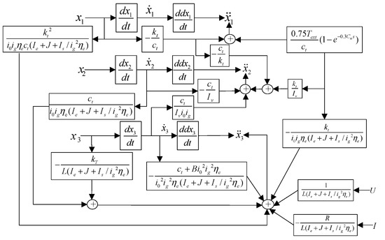
Figure 2.
Vehicle model diagram of the system.
3. Terminal Sliding Mode Controller
For a second-order control system, Equation (23) can be established [29,30,31] as follows:
The electric vehicle tractor model is established as the equation of state [Equation (24)], as follows:
The system state nonlinear function is derived as follows:
The unknown controlled object uncertainty is expressed as follows:
The system state nonlinear function is expressed as
The external disturbance of the controlled object is expressed as
The controller design block diagram is shown in Figure 3.
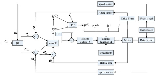
Figure 3.
Controller design block diagram.
3.1. Design of the Terminal Sliding Modulus
The full vehicle model system status = is tracked to derive the desired state formula [Equation (29)] within a limited time, as follows:
The error vector is defined as
The sliding surface designed is expressed as
where Q(t) is a nonlinear sliding surface function.
From the previously presented equations, m = rank (b) = 1, n = 2, C = [C1 C2], Q(t) = CP(t)
, P(t) is a function of order n that can be differentiated, , and ; thus, C = [C1 C2] = [4 1].
Given that the equation of state has three inputs and two outputs, the sliding surface is expressed as follows:
To derive and meet the conditions of Hypothesis 1 [3], the following function is selected:
When 0 ≤ t ≤ T, the function is expressed as follows:
When t ≥ T, the function is expressed as follows:
The expressions of and are derived in a similar manner. According to the conditions of Hypothesis 1, when t = T, = 0, = 0, and = 0, the three equations of parameters are obtained as follows:
The following parameters are also obtained:
The resulting parameter is substituted into the previously presented expression to determine the terminal sliding surface of the second-order system.
3.2. Terminal Sliding Mode Controller Design
To ensure that the tracking error converges on the sliding surface of in any finite time, Equation (32) is used to derive the following expression:
The Lyapunov function is derived as follows:
where V is the Lyapunov function.
If the motion trajectory is required to reach the sliding mode switching surface within a limited time and its arrival condition is < 0, then
Therefore, the controller is designed as follows:
where K is a normal number.
Substituting Equation (42) into Equation (41) yields the following:
Notably, the initial state is on the sliding surface because < 0 ensures the stability of the system. The continuous function vector is used instead of to reduce chattering.
where is a normal number.
Substituting Equations (44) and (45) into Equation (43) yields the following control function:
4. Simulation and Experiment
4.1. Simulation
The sliding mode variable algorithm design is completed. MATLAB/Simulink simulates the state equation of the electric tractor’s complete vehicle equation and the actual operation of the electric tractor to ensure the correctness of the design and practicality of the system. In conducting the analysis, given that the field load is mainly in the form of step, pyrotechnic, sinusoidal, straight line, ramp, and pulse signals during the actual operation, this study uses step, sinusoidal, and ramp signals as examples to assign signals to intermediate variable motors. Angular and driving angular velocities are used to validate the designed model.
The control subroutines are written using the S-function of Simulink modeling. The system parameters in the simulation experiment are kt = 25; Ct = 6; KT = 1.4; Iv = 0.006 kg·m2; Ie = 0.005 kg·m2; Is = 0.004 kg·m2; ηe = 0.95; B = 0.0008 N·m·s/rad; L = 8.5e − 3H; R = 2.875 Ω; and Text = 3500 N·m.
- (1)
- Make the system’s position instruction relative rotation , drive wheel angular speed , and motor angular speed . Continuous functions are used to reduce chattering. and . The simulation results are shown in Figure 4.
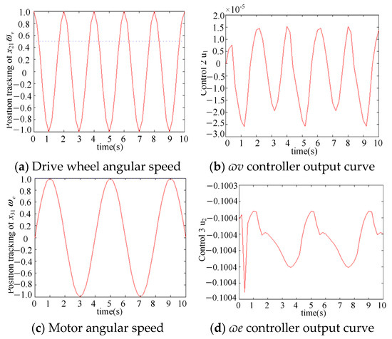 Figure 4. Output of the system state control function simulation.
After stabilization, the simulation result of the control output for the drive wheel angular velocity is floating, but the range of the floating value is to . The simulation result of the control input for the motor angular velocity is also floating, but the floating value is always approximately −1.004. Thus, convergence and chattering are considered to have been eliminated.
- (2)
- Make the system’s position instruction relative rotation , drive wheel angular speed , and motor angular speed . Continuous functions are used to reduce chattering. and . The simulation results are shown in Figure 5.
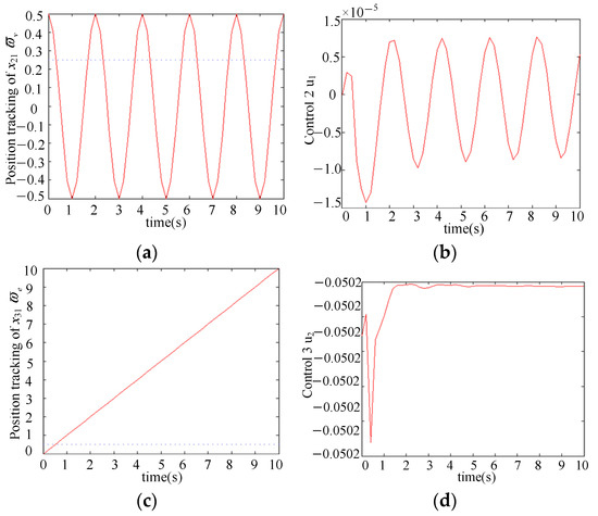 Figure 5. Output of the system state control function simulation. (a) Drive wheel angular speed. (b) ϖv controller output curve. (c) Motor angular speed. (d) ϖe controller output curve.
After stabilization, the simulation result of the control output for the drive wheel angular velocity is floating, but the range of the floating value is to , and the simulation result of the control input for the motor angular velocity is also floating. However, the floating value is always approximately −0.0502. Thus, convergence and chattering are considered to have been eliminated.
Under the control function, the initial state of the position command rapidly tracks the position function. According to the simulation diagram, the control function can rapidly adjust the acceleration of the motor and the drive wheel when the position error approaches the sliding surface. The control function tends to be close to 0, ensuring that the electric tractor runs at a given speed. The simulation diagram shows that this algorithm converges and eliminates chattering.
- (3)
- Simulate the actual situation in the field and compare the sliding mode variable algorithm with the PID algorithm. Set the brushless DC motor start as Tout = 0 N·m and the motor speed = 1000 rad/min. When t = 0.6 s, sudden load torque Tout = 8 N·m. Figure 6 shows the motor torque simulation diagram, and Figure 7 shows the motor speed simulation diagram. The PID overshoot is large, the fluctuations are severe, and the terminal is accurately adjusted.
 Figure 6. Motor torque simulation.
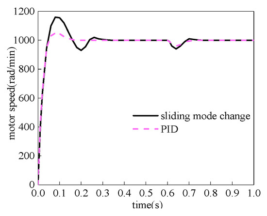 Figure 7. Motor speed simulation.
The torque diagram shown in Figure 6 indicates that the sliding mode can be adjusted rapidly and tends to be stable. The results of the PID algorithm show the occurrence of an overshoot during the entire process. Large fluctuations are observed above and below the stable value. Moreover, a stable state cannot be formed.
Figure 7 shows the motor speed simulation diagram with the motor speed value set to 1000 rad/min. The adaptive terminal sliding mode algorithm can rapidly stabilize the set value when the motor starts. Moreover, the PID algorithm forms a large overshoot because of dynamic reasons. The time for balancing the overshoot is 0.3 s. After 0.6 s interference, the adaptive terminal sliding mode control overshoot is 3%, and the response time in the adjustment of 0.1 s tends to be stable. The PID speed overshoot is 6%, and the response time in the adjustment of 0.16 s tends to be stable.
The comparison of the two algorithms shows that the electromagnetic torque of the control system under the adaptive terminal sliding mode variable modulation exhibits less fluctuation whether under sudden load change or speed change, which can speed up the response speed, reduce the overshoot, and be affected by external influences. When the system can rapidly return to a stable state, the control effect is better than that of PID.
4.2. Test Analysis
In designing and developing a constant speed controller, a test stand is built to verify the reliability of the control algorithm. The controller test bench is shown in Figure 8.
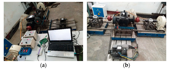
Figure 8.
System test bench. (a) Side test bench. (b) Front test bench.
The experimental steps for simulating load mutations are as follows: (a) adjust the manual tension meter not to load the magnetic powder brake, so that the left and right wheel loads are 0; (b) start the motor, press the forward button (set the forward motor speed to 1000 rad/min); (c) add the load of 50 N·m to the right wheel and observe the changes of the torque, speed of the motor, and the right drive wheel; (d) press the neutral button to turn off the motor and end the test procedure. The experimental results are shown in Figure 9.
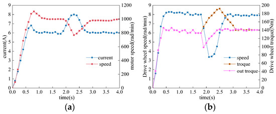
Figure 9.
System sliding modulation algorithm under the control of an abrupt load curve. (a) Motor speed and current. (b) Drive wheel speed and torque.
The motor speed is set to 1000 rad/min, and the time is set to 1 s to achieve a stable state. The experimental drive wheel speed is 8.1 rad/min. An abrupt load of 50 N·m is added at 2 s and eliminated at 2.3 s during the implementation of the adaptive terminal algorithm. Given the abrupt change in drive wheel speed, the control algorithm is used to increase the current (Te, the electromagnetic torque) to ensure that the drive wheel speed remains constant. The motor speed is decreased to counteract the effects of the abrupt load. After the load is eliminated, the motor speed and drive wheel speed recovers under the action of the control algorithm. The drive wheel eliminates disturbances for 1.1 s.
5. Conclusions
In this paper, the constant speed intelligent control system of electric tractor is taken as the research object, and a constant speed control method is proposed based on the sudden change load encountered by electric tractors in field conditions. The main research results are as follows:
- (1)
- Based on the correlation parameters among modules, using the relative angle of the transmission output shaft, driving wheel velocity, mechanical angular velocity of motor as intermediate variables, we obtained the driving wheel velocity and mechanical angular velocity of motor for the output of three input and two output state equation;
- (2)
- Aiming at the vehicle speed, the sliding mode surface is designed using ”linear + nonlinear” features, and the adaptive terminal sliding mode variable control function is designed, so as to realize the control ability of adaptive online adjustment;
- (3)
- The simulation and test results show that, compared with the PID algorithm, the adaptive terminal sliding mode variable algorithm can quickly eliminate the voltage deviation, and achieve a fast response speed and short overshoot time. The tracking error on the sliding mode plane can converge to zero in a limited time. The control accuracy is better, and it has good robustness.
Author Contributions
S.Y. contributed to conceptualization, methodology, and writing—original draft of the paper; P.M. contributed to conceptualization, methodology, supervision, and writing—review of the paper; W.L. contributed to writing—review and editing. All authors have read and agreed to the published version of the manuscript.
Funding
This work was supported by the Science and Technology Development Project in Henan Province (232102241042).
Institutional Review Board Statement
Not applicable.
Informed Consent Statement
Not applicable.
Data Availability Statement
The authors confirm that the data supporting the findings of this study are available within the article.
Conflicts of Interest
The authors declare no conflict of interest.
References
- Wu, Z.; Xie, B.; Li, Z.; Chi, R.; Ren, Z.; Du, Y.; Inoue, E.; Mitsuoka, M.; Okayasu, T.; Hirai, Y. Modelling and verification of driving torque management for electric tractor: Dual-mode driving intention interpretation with torque demand restriction. Biosyst. Eng. 2019, 182, 65–83. [Google Scholar] [CrossRef]
- Liu, J.; Xia, C.; Jiang, D.; Sun, Y. Development and testing of the power transmission system of a crawler electric tractor for greenhouses. Appl. Eng. Agric. 2020, 36, 797–805. [Google Scholar] [CrossRef]
- Jin, X.; Dai, S.; Liang, J. Adaptive constrained formation-tracking control for a tractor-trailer mobile robot team with multiple constraints. IEEE Trans. Autom. 2023, 68, 1700–1707. [Google Scholar] [CrossRef]
- Tufail, M.; Iqbal, J.; Tiwana, M.I.; Alam, M.S.; Khan, Z.A.; Khan, M.T. Identification of tobacco crop based on machine learning for a precision agricultural sprayer. IEEE Access 2021, 9, 23814–23825. [Google Scholar] [CrossRef]
- Xie, B.; Wang, S.; Wu, X.; Wen, C.; Zhang, S.; Zhao, X. Design and hardware-in-the-loop test of a coupled drive system for electric tractor. Biosyst. Eng. 2022, 216, 165–185. [Google Scholar] [CrossRef]
- Cheng, Z.; Lu, Z. Research on the PID control of the ESP system of tractor based on improved AFSA and improved SA. Comput. Electron. Agric. 2018, 148, 142–147. [Google Scholar] [CrossRef]
- Li, Z.; Chen, H.; Liu, H.; Wang, P.; Gong, X. Integrated longitudinal and lateral vehicle stability control for extreme conditions with safety dynamic requirements analysis. IEEE Trans. Intell. Transp. Syst. 2022, 23, 19285–19298. [Google Scholar] [CrossRef]
- Zine, W.; Makni, Z.; Monmasson, E.; Idkhajine, L.; Condamin, B. Interests and limits of machine learning-based neural networks for rotor position estimation in EV traction drives. IEEE Trans. Ind. Inform. 2018, 14, 1942–1951. [Google Scholar] [CrossRef]
- Dzmitry, S.; Valentin, I.; Klaus, A.; Tomoki, E.; Hiroyuki, F.; Hiroshi, F.; Leonid, F. Wheel slip control for the electric vehicle with in-wheel motors: Variable structure and sliding mode methods. IEEE Trans. Ind. Electron. 2022, 67, 8535–8544. [Google Scholar]
- Sunusi, I.; Zhou, J.; Sun, C.; Wang, Z.; Zhao, J.; Wu, Y. Development of online adaptive traction control for electric robotic tractors. Energies 2021, 14, 3394. [Google Scholar] [CrossRef]
- Incremona, G.; Rubagotti, M.; Ferrara, A. Sliding mode control of constrained nonlinear systems. IEEE Trans. Autom. Control 2017, 62, 2965–2972. [Google Scholar] [CrossRef]
- Choi, H. Robust Stabilization of uncertain fuzzy-time-delay systems using sliding-mode-control approach. IEEE Trans. Fuzzy Syst. 2010, 18, 979–984. [Google Scholar] [CrossRef]
- Zhang, Y.; Zhang, Q.; Zhang, J. Sliding mode control for fuzzy singular systems with time delay based on vector integral sliding mode surface. IEEE Trans. Fuzzy Syst. 2020, 28, 768–782. [Google Scholar] [CrossRef]
- Wang, Y.; Wang, Z. Model free adaptive fault-tolerant consensus tracking control for multiagent systems. Neural Comput. Appl. 2022, 34, 10065–10079. [Google Scholar] [CrossRef]
- Nima, L.; Reza, S. Spacecraft attitude control: Application of fine trajectory linearization control. Adv. Space Res. 2021, 68, 3663–3676. [Google Scholar]
- Ding, S.; Liu, L.; Park, J. A novel adaptive nonsingular terminal sliding mode controller design and its application to active front steering system. Int. J. Robust Nonlinear Control 2019, 29, 4250–4269. [Google Scholar] [CrossRef]
- Hou, H.; Yu, X.; Xu, L.; Rsetam, K.; Cao, Z. Finite-time continuous terminal sliding mode control of servo motor systems. IEEE Trans. Ind. Electron. 2020, 67, 5647–5656. [Google Scholar] [CrossRef]
- Kamal, R.; Cao, Z.; Man, Z. Cascaded-extended-state-observer-based sliding-mode control for underactuated flexible joint robot. IEEE Trans. Ind. Electron. 2020, 67, 10822–10832. [Google Scholar]
- Kamal, R.; Cao, Z.; Man, Z. Design of robust terminal sliding mode control for underactuated flexible joint robot. IEEE Trans. Syst. 2022, 52, 4272–4273. [Google Scholar]
- Qi, W.; Park, J.H.; Zong, G.; Cao, J.; Cheng, J. A fuzzy lyapunov function approach to positive l_1 observer design for positive fuzzy semi-markovian switching systems with its application. IEEE Trans. Syst. Man Cybern. Syst. 2019, 51, 775–785. [Google Scholar] [CrossRef]
- Yoo, B.; Ham, W. Adaptive fuzzy sliding mode control of nonlinear system. IEEE Trans. Fuzzy Syst. 1998, 6, 315–321. [Google Scholar]
- Simon, K.; Christoph, M. Nonlinear modelling and control of a power smoothing system for a novel wave energy converter prototype. Sustainability 2022, 14, 13708. [Google Scholar]
- Carter, R.; Cruden, A.; Hall, P.J.; Zaher, A.S. An improved lead–acid battery pack model for use in power simulations of electric vehicles. IEEE Trans. Energy Convers. 2012, 27, 21–28. [Google Scholar] [CrossRef]
- Offer, G.J.; Howey, D.; Contestabile, M.; Clague, R.; Brandon, N.P. Comparative analysis of battery electric, hydrogen fuel cell and hybrid vehicles in a future sustainable road transport system. Energy Policy 2010, 38, 24–29. [Google Scholar] [CrossRef]
- Mohamadabadi, H.; Tichkowsky, G.; Kumar, A. Development of a multi-criteria assessment model for ranking of renewable and non-renewable transportation fuel vehicles. Energy 2009, 34, 112–125. [Google Scholar] [CrossRef]
- Liang, C.; Su, J. A new approach to the design of a fuzzy sliding mode controller. Fuzzy Sets Syst. 2003, 139, 111–124. [Google Scholar] [CrossRef]
- Yang, Z.; Qin, D.; Sun, D. Parameter design and dynamic simulation of powertrain for electric vehicles. J. Chongqing Univ. 2002, 25, 19–22. [Google Scholar]
- Li, T.; Xie, B.; Li, Z.; Li, J. Design and optimization of a dual-input coupling powertrain system: A case study for electric tractors. Appl. Sci. 2020, 10, 1608. [Google Scholar] [CrossRef]
- Cardim, R.; Teixeira, M.C.; Assunção, E.; Ribeiro, J.M.; Covacic, M.R.; Gaino, R. Robust switched control based on strictly positive real systems and variable structure control techniques. Int. J. Adapt. Control Signal Process. 2016, 30, 1244–1268. [Google Scholar] [CrossRef]
- Zhao, G.; Peng, X. Variable structure control strategy research on regenerative braking for a brushless dc motor driven electric bus cruising downhill. J. Adv. Manuf. Syst. 2014, 13, 223–236. [Google Scholar] [CrossRef]
- Xuan, S.; Song, C.; Meng, G. ABS sliding mode variable structure control based on index reaching law. Adv. Mater. Res. 2014, 3140, 439–443. [Google Scholar] [CrossRef]


Disclaimer/Publisher’s Note: The statements, opinions and data contained in all publications are solely those of the individual author(s) and contributor(s) and not of MDPI and/or the editor(s). MDPI and/or the editor(s) disclaim responsibility for any injury to people or property resulting from any ideas, methods, instructions or products referred to in the content. |
© 2023 by the authors. Licensee MDPI, Basel, Switzerland. This article is an open access article distributed under the terms and conditions of the Creative Commons Attribution (CC BY) license (https://creativecommons.org/licenses/by/4.0/).