
V2G Scheduling of Electric Vehicles Considering Wind Power Consumption


Abstract
:1. Introduction
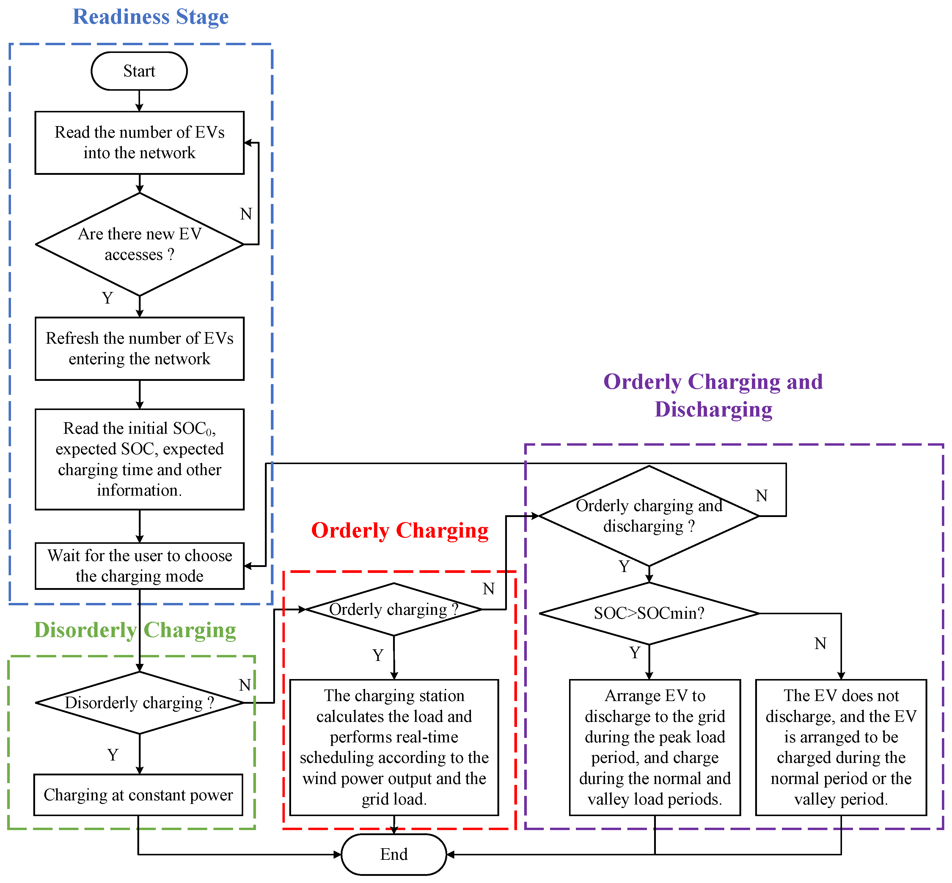
2. Orderly Charging and Discharging of EVs in Mountainous Cities
3. Charging and Discharging Model of EV in Mountainous Cities
3.1. Objective Function
3.2. Constraint Conditions
4. Model Solution
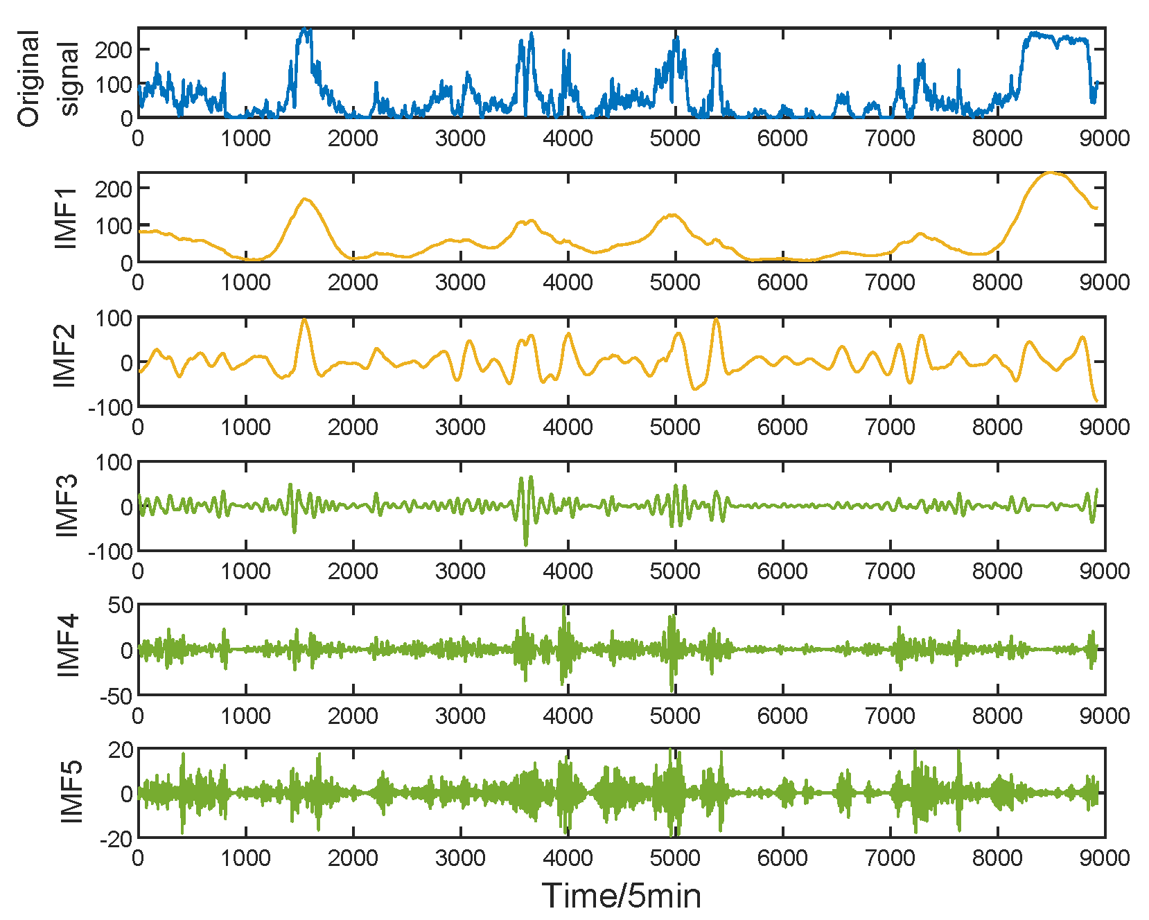
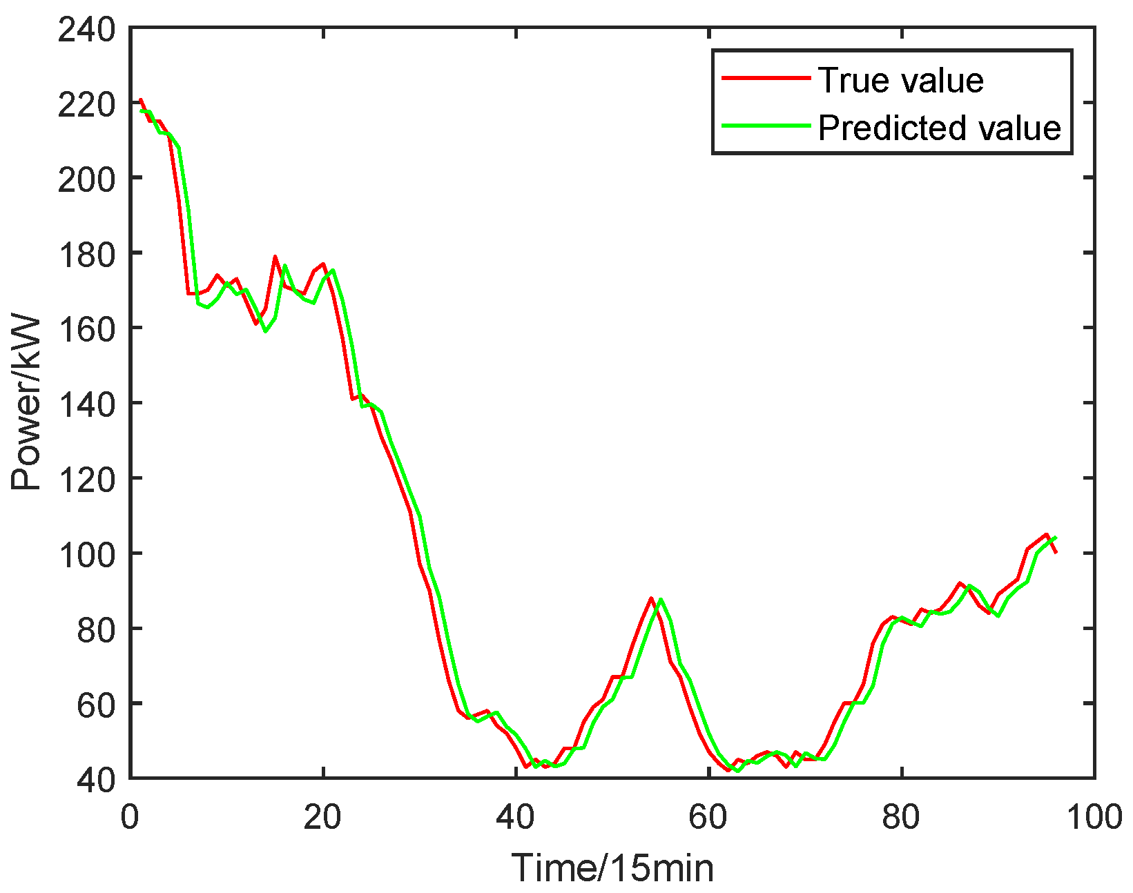
4.1. WP Prediction Model
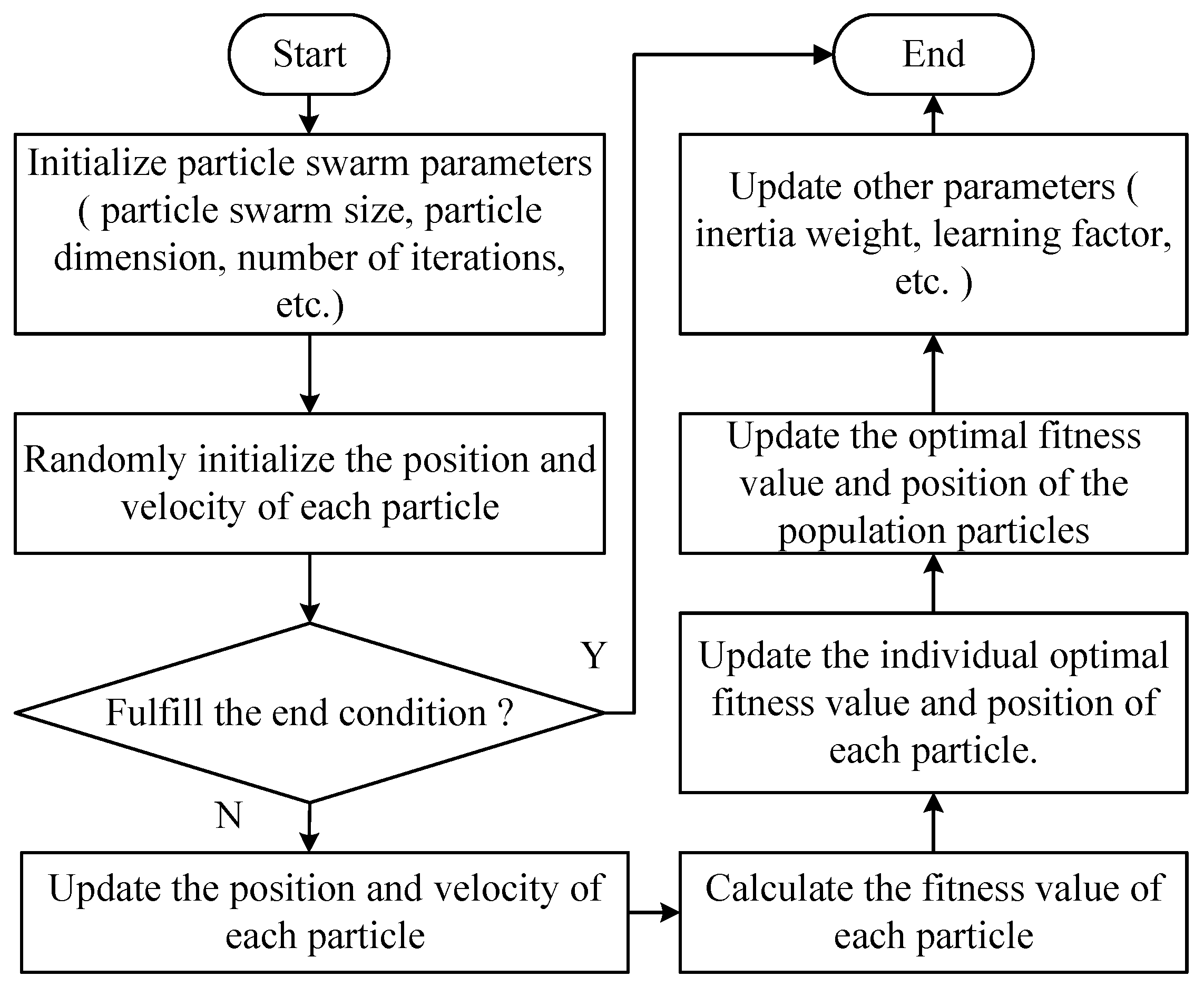
4.2. Particle Swarm Optimization Algorithm Solution
- Initialize particle swarm parameters, such as particle swarm size, particle dimension, number of iterations, etc.
- Initialize the position and velocity of each particle.
- Determine whether the end condition is satisfied. If the end condition is satisfied, the algorithm ends and the optimal solution is obtained. If the conditions are not met, the following steps will continue.
- Update the position and velocity of the particle, and calculate the fitness value of the particle.
- Then, the individual optimal fitness value and position of each particle and the optimal fitness value and position of the group particles are updated.
- Update other parameters such as inertia weight and learning factor.
- Obtain the final result.
4.2.1. Dynamic Weight Setting
4.2.2. Dynamic Learning Factors Settings
5. Example Analysis
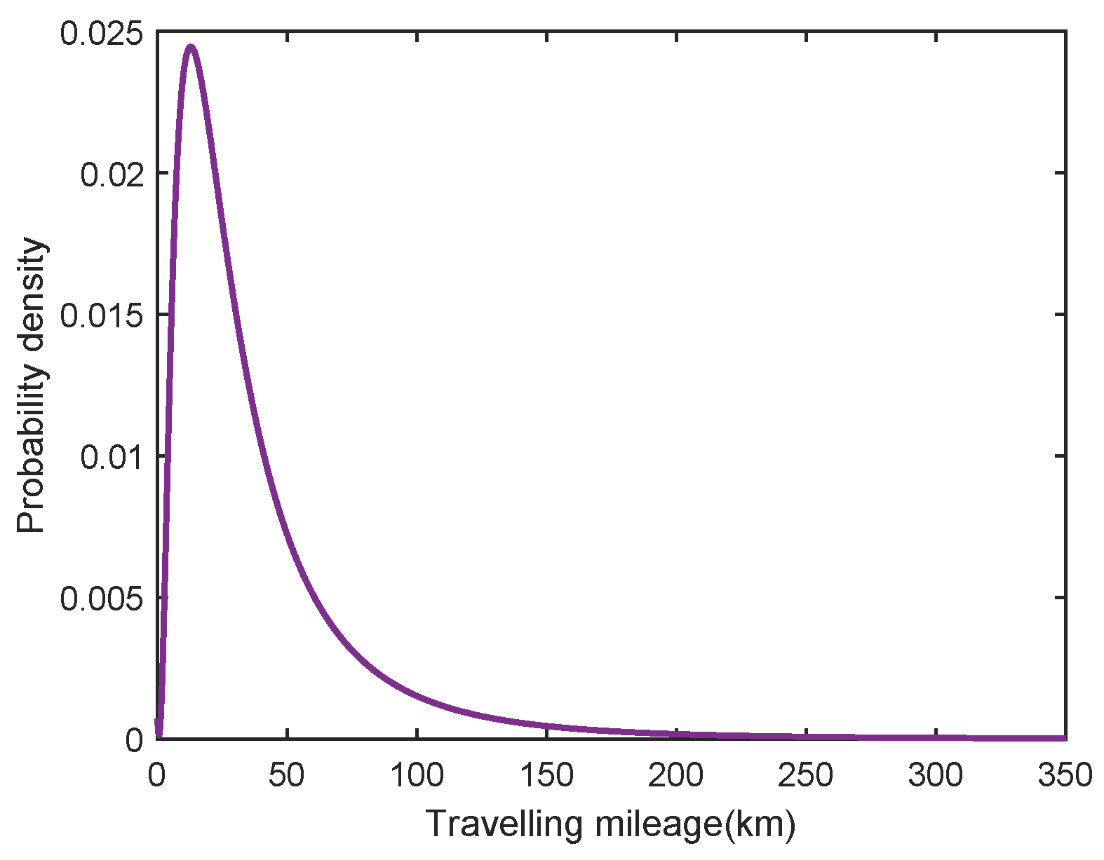
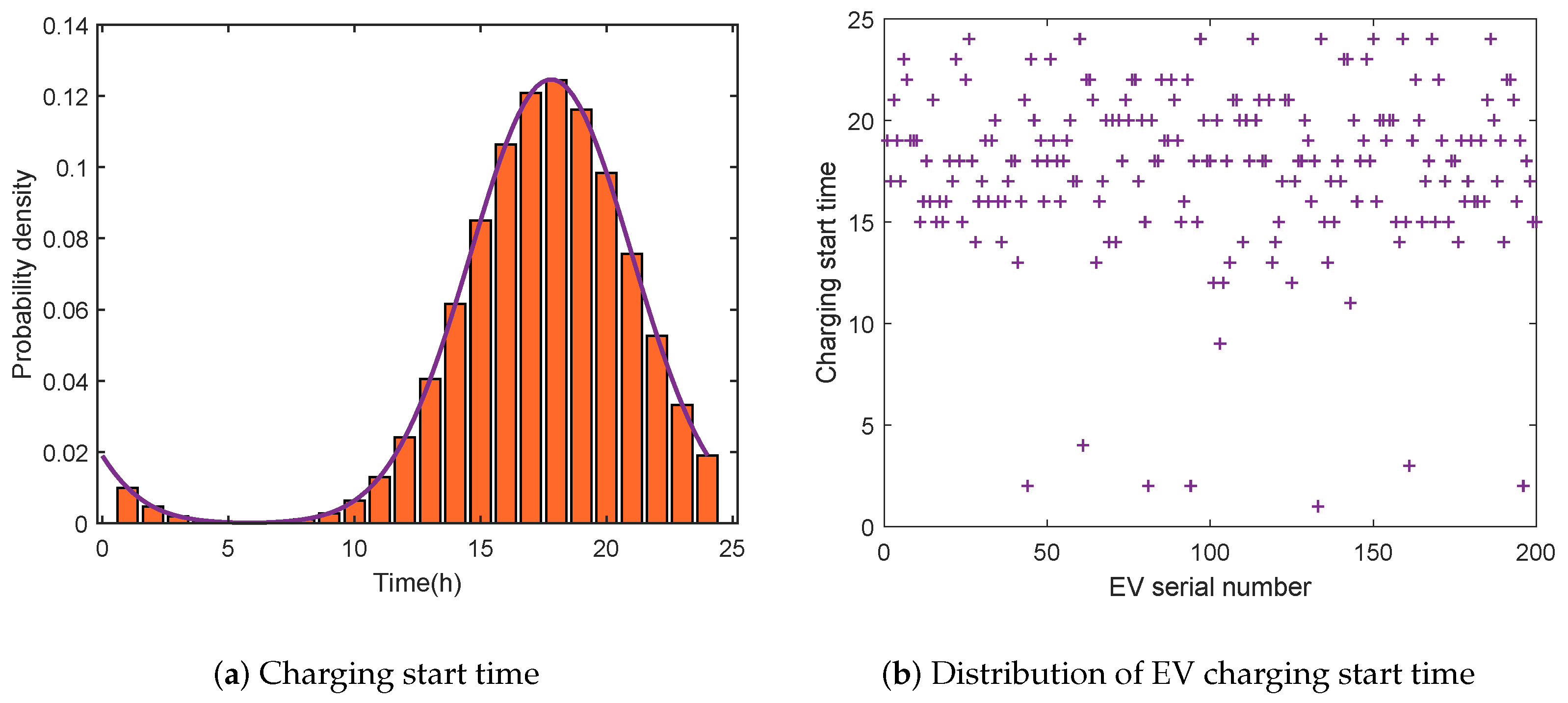
- Taking a residential area in Chongqing, China, as an example, it is set that there are 200 EVs in the area, the model is BYD e6, the battery capacity is 82 kWh, the charging mode is conventional slow charging, the power is 7 kW, and the battery charging and discharging efficiency is 0.9. The maximum load capacity of the transformer in the residential area is 5087 kW. Through Monte Carlo simulation analysis of user travel patterns, it is basically selected to go home to charge after work and finish charging before going to work the next day. In this paper, 10% random loads are set; that is, 20 EVs are arranged to carry out orderly charging and discharging scheduling during the working hours of the community.
- After the charging mode is selected for the EV connected to the power grid, the charging station will dispatch the EV according to the dynamic electric price. When the expected SOC set by the user is reached, the charging will stop.
- EV participates in V2G voluntarily, and the users who are willing to respond to the scheduling sign an agreement with the grid to implement the scheduling arrangement. This paper analyzes the objective functions with 30%, 60%, and 100% responsiveness.
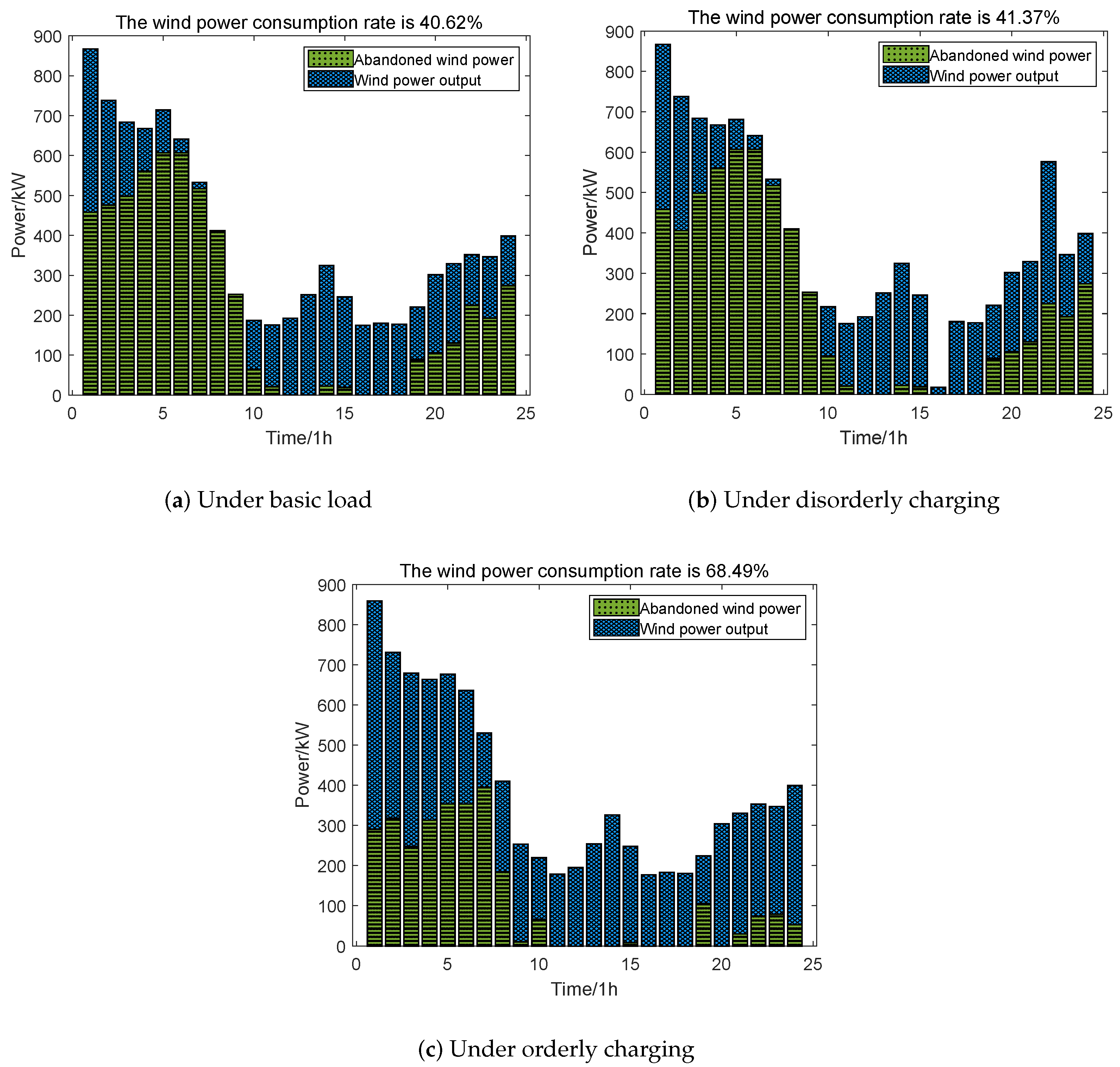
5.1. Do Not Participate in V2G Scheduling
5.2. V2G Different Responsiveness Scheduling
6. Conclusions
Author Contributions
Funding
Data Availability Statement
Conflicts of Interest
References
- Li, C.; Zhang, L.; Ou, Z.; Wang, Q.; Zhou, D.; Ma, J. Robust model of electric vehicle charging station location considering renewable energy and storage equipment. Energy 2022, 238, 121713. [Google Scholar] [CrossRef]
- Hao, Y.; Dong, L.; Liang, J.; Liao, X.; Wang, L.; Shi, L. Power forecasting-based coordination dispatch of PV power generation and electric vehicles charging in microgrid. Renew. Energy 2020, 155, 1191–1210. [Google Scholar] [CrossRef]
- Ren, X.; Zeng, Y.; Sun, Z.; Wang, J. A Novel Day Optimal Scheduling Strategy for Integrated Energy System including Electric Vehicle and Multisource Energy Storage. Int. Trans. Electr. Energy Syst. 2023, 2023, 3880254. [Google Scholar] [CrossRef]
- Wu, S.; Pang, A. Optimal scheduling strategy for orderly charging and discharging of electric vehicles based on spatio-temporal characteristics. J. Clean. Prod. 2023, 392, 136318. [Google Scholar] [CrossRef]
- Kazerani, M.; Tehrani, K. Grid of hybrid AC/DC microgrids: A new paradigm for smart city of tomorrow. In Proceedings of the 2020 IEEE 15th International Conference of System of Systems Engineering (SoSE), Budapest, Hungary, 2–4 June 2020; pp. 175–180. [Google Scholar]
- Zhang, L.; Yin, Q.; Zhang, Z.; Zhu, Z.; Lyu, L.; Hai, K.L.; Cai, G. A wind power curtailment reduction strategy using electric vehicles based on individual differential evolution quantum particle swarm optimization algorithm. Energy Rep. 2022, 8, 14578–14594. [Google Scholar] [CrossRef]
- Yu, Z.; Gong, P.; Wang, Z.; Zhu, Y.; Xia, R.; Tian, Y. Real-time control strategy for aggregated electric vehicles to smooth the fluctuation of wind-power output. Energies 2020, 13, 757. [Google Scholar] [CrossRef]
- Mingqiang, C.; Jianfei, G.; Guogang, C.; Fei, B. Research on orderly charging strategy of micro-grid electric vehicles in V2G model. Power Syst. Prot. Control 2020, 48, 141–148. [Google Scholar]
- Liu, Z.; Xiao, Z.; Wu, Y.; Hou, H.; Xu, T.; Zhang, Q.; Xie, C. Integrated optimal dispatching strategy considering power generation and consumption interaction. IEEE Access 2020, 9, 1338–1349. [Google Scholar] [CrossRef]
- Pan, Y.; Wang, W.; Li, Y.; Zhang, F.; Sun, Y.; Liu, D. Research on cooperation between wind farm and electric vehicle aggregator based on A3C algorithm. IEEE Access 2021, 9, 55155–55164. [Google Scholar] [CrossRef]
- Liu, D.; Wang, L.; Wang, W.; Li, H.; Liu, M.; Xu, X. Strategy of large-scale electric vehicles absorbing renewable energy abandoned electricity based on master-slave game. IEEE Access 2021, 9, 92473–92482. [Google Scholar] [CrossRef]
- Nourianfar, H.; Abdi, H. Economic emission dispatch considering electric vehicles and wind power using enhanced multi-objective exchange market algorithm. J. Clean. Prod. 2023, 415, 137805. [Google Scholar] [CrossRef]
- Hou, H.; Xue, M.; Xu, Y.; Xiao, Z.; Deng, X.; Xu, T.; Liu, P.; Cui, R. Multi-objective economic dispatch of a microgrid considering electric vehicle and transferable load. Appl. Energy 2020, 262, 114489. [Google Scholar] [CrossRef]
- Wang, H.; Ma, H.; Liu, C.; Wang, W. Optimal scheduling of electric vehicles charging in battery swapping station considering wind-photovoltaic accommodation. Electr. Power Syst. Res. 2021, 199, 107451. [Google Scholar] [CrossRef]
- Yin, W.J.; Ming, Z.F. Electric vehicle charging and discharging scheduling strategy based on local search and competitive learning particle swarm optimization algorithm. J. Energy Storage 2021, 42, 102966. [Google Scholar] [CrossRef]
- Hu, Y.; Zhang, M.; Wang, K.; Wang, D. Optimization of orderly charging strategy of electric vehicle based on improved alternating direction method of multipliers. J. Energy Storage 2022, 55, 105483. [Google Scholar] [CrossRef]
- Habib, H.U.R.; Waqar, A.; Hussien, M.G.; Junejo, A.K.; Jahangiri, M.; Imran, R.M.; Kim, Y.S.; Kim, J.H. Analysis of microgrid’s operation integrated to renewable energy and electric vehicles in view of multiple demand response programs. IEEE Access 2022, 10, 7598–7638. [Google Scholar] [CrossRef]
- Cai, L.; Zhang, Q.; Dai, N.; Xu, Q.; Gao, L.; Shang, B.; Xiang, L.; Chen, H. Optimization of Control Strategy for Orderly Charging of Electric Vehicles in Mountainous Cities. World Electr. Veh. J. 2022, 13, 195. [Google Scholar] [CrossRef]
- Zhou, S.; Gu, B.; Zhang, X. Optimal Planning for Charging Facilities Considering Spatial and Temporal Characteristics of Mountainous Cities. Power Syst. Technol. 2020, 44, 2229–2237. [Google Scholar]
- Tian, J.; Lv, Y.; Zhao, Q.; Gong, Y.; Li, C.; Ding, H.; Yu, Y. Electric vehicle charging load prediction considering the orderly charging. Energy Rep. 2022, 8, 124–134. [Google Scholar] [CrossRef]
- Bayati, M.; Abedi, M.; Farahmandrad, M.; Gharehpetian, G.B.; Tehrani, K. Important technical considerations in design of battery chargers of electric vehicles. Energies 2021, 14, 5878. [Google Scholar] [CrossRef]
- He, W.; Xianda, L.; Yuhan, P.; Jing, B.; Zhongshu, Y. Orderly charging and discharging strategy of electric vehicle considering spatio-temporal characteristic and time cost. Electr. Power Autom. Equip. 2022, 42, 86–91+133. [Google Scholar]
- Mori, Y.; Wakao, S.; Ohtake, H.; Takamatsu, T.; Oozeki, T. Area day-ahead photovoltaic power prediction by just-in-time modeling with meso-scale ensemble prediction system. Electr. Eng. Jpn. 2023, 143, e23426. [Google Scholar] [CrossRef]
- Luo, X.; Zhang, D.; Zhu, X. Deep learning based forecasting of photovoltaic power generation by incorporating domain knowledge. Energy 2021, 225, 120240. [Google Scholar] [CrossRef]
- Wang, Z.; Wang, X.; Liu, W. Genetic least square estimation approach to wind power curve modelling and wind power prediction. Sci. Rep. 2023, 13, 9188. [Google Scholar] [CrossRef]
- Chen, G.; Zhang, T.; Qu, W.; Wang, W. Photovoltaic Power Prediction Based on VMD-BRNN-TSP. Mathematics 2023, 11, 1033. [Google Scholar] [CrossRef]
- Jency, W.; Judith, J. Homogenized Point Mutual Information and Deep Quantum Reinforced Wind Power Prediction. Int. Trans. Electr. Energy Syst. 2022, 2022, 3686786. [Google Scholar] [CrossRef]
- Feng, C.; Yi, Y.; Jingyou, X.; Jie, Y.; Ke, C.; Tiandong, Z.; Lufang, G.; Zijian, Z.; Po, H. Prediction method of wind power output based on a Bayes-LSTM network. Power Syst. Prot. Control 2023, 51, 170–178. [Google Scholar]
- Tarek, Z.; Shams, M.Y.; Elshewey, A.M.; El-kenawy, E.S.M.; Ibrahim, A.; Abdelhamid, A.A.; El-dosuky, M.A. Wind Power Prediction Based on Machine Learning and Deep Learning Models. Comput. Mater. Contin. 2023, 75, 715–732. [Google Scholar] [CrossRef]
- Zou, Y.; Zhao, J.; Ding, D.; Miao, F.; Sobhani, B. Solving dynamic economic and emission dispatch in power system integrated electric vehicle and wind turbine using multi-objective virus colony search algorithm. Sustain. Cities Soc. 2021, 67, 102722. [Google Scholar] [CrossRef]
- Zeynali, S.; Nasiri, N.; Marzband, M.; Ravadanegh, S.N. A hybrid robust-stochastic framework for strategic scheduling of integrated wind farm and plug-in hybrid electric vehicle fleets. Appl. Energy 2021, 300, 117432. [Google Scholar] [CrossRef]
- Liu, W.; Wang, Z.; Yuan, Y.; Zeng, N.; Hone, K.; Liu, X. A novel sigmoid-function-based adaptive weighted particle swarm optimizer. IEEE Trans. Cybern. 2019, 51, 1085–1093. [Google Scholar] [CrossRef]
- Yang, Y.; Duan, W.; Wang, W.; Zhang, X.; Peng, X.; Han, Q.; Li, Y.; Li, S.; Gao, S. EV Senseless Orderly Charging Technology for High User Participation Rate in Residential Area. World Electr. Veh. J. 2022, 13, 126. [Google Scholar] [CrossRef]
- Song, Z.; Liu, B.; Cheng, H. Adaptive particle swarm optimization with population diversity control and its application in tandem blade optimization. Proc. Inst. Mech. Eng. Part C J. Mech. Eng. Sci. 2019, 233, 1859–1875. [Google Scholar] [CrossRef]
- Xu, L.; Song, B.; Cao, M. An improved particle swarm optimization algorithm with adaptive weighted delay velocity. Syst. Sci. Control Eng. 2021, 9, 188–197. [Google Scholar] [CrossRef]
- Flori, A.; Oulhadj, H.; Siarry, P. QUAntum Particle Swarm Optimization: An auto-adaptive PSO for local and global optimization. Comput. Optim. Appl. 2022, 82, 525–559. [Google Scholar] [CrossRef]
- Li, W.; Sun, B.; Huang, Y.; Mahmoodi, S. Adaptive complex network topology with fitness distance correlation framework for particle swarm optimization. Int. J. Intell. Syst. 2022, 37, 5217–5247. [Google Scholar] [CrossRef]
- Du, W.; Ma, J.; Yin, W. Orderly charging strategy of electric vehicle based on improved PSO algorithm. Energy 2023, 271, 127088. [Google Scholar] [CrossRef]


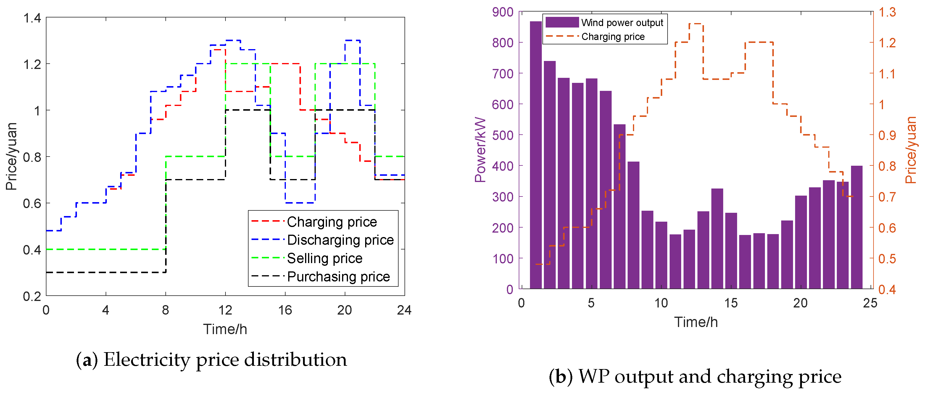
| Time Interval | C (Yuan/kWh) | C (Yuan/kWh) |
|---|---|---|
| Peak period (11:00–14:00, 17:00–21:00) | 1.2 | 1.0 |
| Flat period (7:00–11:00, 14:00–17:00, 21:00–24:00) | 0.8 | 0.7 |
| Valley period (0:00–7:00) | 0.4 | 0.3 |
| Peak Value/(kW) | Valley Value/(kW) | Peak–Valley Difference/(kW) | WP Consumption Rate/(%) | Electricity Sales Benefit Value/Dollar | Growth Rate/(%) | |
|---|---|---|---|---|---|---|
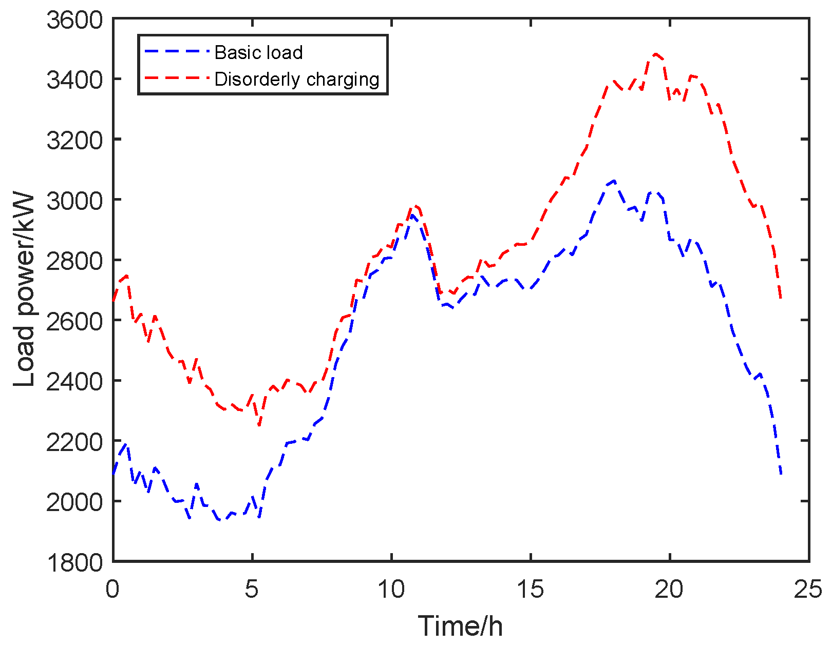
| Basic load | 3062.6 | 1932.0 | 1130.6 | 40.62% | 4173.17 | – |
| Disorderly charging | 3454.7 | 2161.6 | 1293.1 | 41.37% | 7108.04 | 41.8% |
| Orderly charging | 3208.5 | 2394.0 | 814.5 | 68.49% | 8752.70 | 18.8% |
| User Responsiveness | Peak Value/(kW) | Valley Value/(kW) | Peak–Valley Difference/(kW) | WP Consumption Rate/(%) | Growth Rate/(%) | Electricity Sales Benefit Value/Dollar |
|---|---|---|---|---|---|---|
| 30% | 2886.2 | 2002.7 | 883.5 | 72.10% | 1.05% | 7291.26 |
| 60% | 2868.2 | 2102.7 | 765.5 | 81.04% | 9.94% | 6264.77 |
| 100% | 2853.6 | 2214.7 | 638.9 | 92.69% | 11.65% | 4895.98 |
Disclaimer/Publisher’s Note: The statements, opinions and data contained in all publications are solely those of the individual author(s) and contributor(s) and not of MDPI and/or the editor(s). MDPI and/or the editor(s) disclaim responsibility for any injury to people or property resulting from any ideas, methods, instructions or products referred to in the content. |
© 2023 by the authors. Licensee MDPI, Basel, Switzerland. This article is an open access article distributed under the terms and conditions of the Creative Commons Attribution (CC BY) license (https://creativecommons.org/licenses/by/4.0/).
Share and Cite
Shang, B.; Dai, N.; Cai, L.; Yang, C.; Li, J.; Xu, Q. V2G Scheduling of Electric Vehicles Considering Wind Power Consumption. World Electr. Veh. J. 2023, 14, 236. https://doi.org/10.3390/wevj14090236
Shang B, Dai N, Cai L, Yang C, Li J, Xu Q. V2G Scheduling of Electric Vehicles Considering Wind Power Consumption. World Electric Vehicle Journal. 2023; 14(9):236. https://doi.org/10.3390/wevj14090236
Chicago/Turabian StyleShang, Bingjie, Nina Dai, Li Cai, Chenxi Yang, Junting Li, and Qingshan Xu. 2023. "V2G Scheduling of Electric Vehicles Considering Wind Power Consumption" World Electric Vehicle Journal 14, no. 9: 236. https://doi.org/10.3390/wevj14090236