Article

Rolling Bearing Fault Diagnosis Based on Optimized VMD Combining Signal Features and Improved CNN

College of Mechanical and Vehicular Engineering, Changchun University, Changchun 130022, China
*
Author to whom correspondence should be addressed.
World Electr. Veh. J. 2024, 15(12), 544; https://doi.org/10.3390/wevj15120544
Submission received: 13 October 2024 / Revised: 13 November 2024 / Accepted: 20 November 2024 / Published: 22 November 2024

Abstract

:
Aiming at the problem that the vibration signals of rolling bearings in high-speed rail traction motors are often affected by noise when they are in a fault state, which makes it very difficult to extract the fault features during fault diagnosis and causes obstruction in fault classification. The article proposes a rolling bearing fault diagnosis based on optimized variational mode decomposition (VMD) combined with signal features and an improved convolutional neural network (CNN). The golden jackal optimization (GJO) algorithm is employed to optimize the key parameters of the VMD, enabling effective signal decomposition. The decomposed signals are then filtered and reconstructed using criteria based on kurtosis and interrelationship measures. The time-domain features of the reconstructed signals are computed, and the feature vectors are constructed, which are used as inputs to the deep learning network; the CNN combined with the support vector machine (SVM) network model is used for the extraction of the features and the classification of the faults. The experimental results show that the method can effectively extract fault features in noise-covered signals, and the accuracy is also significantly improved compared with traditional methods.

1. Introduction

Rolling bearings represent a crucial element in the functionality of mechanical equipment, with a diverse range of applications, and in the actual production process, bearings may fail due to friction, wear and tear, the lubrication not being timely, and so on [1]. If we cannot find out in time if it has failed, not only leads to a decline in the use of, performance, and life of the bearings, but also may even cause all equipment fail [2], which will produce serious economic losses [3]. Therefore, the timely and effective diagnosis of faults in rolling bearings is of paramount importance in order to guarantee the safety of industrial production and to ensure the economic benefits that derive from it [4].
Rolling bearing failure, signals containing complex features, as well as the presence of a fault frequency modulation signal [5], alongside the poor working environments and the fault signal being covered by noise, results in our acquisition of the vibration signal becoming complex and difficult to analyze, which leads to the fault characteristics being difficult to extract [6]. To effectively extract the fault characteristics from the vibration signal, the signal noise reduction process becomes particularly important [7]. Fault diagnosis methods in noisy environments include several approaches such as signal processing, feature extraction, and anti-noise machine learning models. Currently, the most commonly employed signal processing methods include wavelet transform (WT), Empirical Mode Decomposition (EMD), and VMD. Band-pass filtering and wavelet transform techniques can effectively suppress noise in a specific frequency range [8]. Among them, wavelet transforms can decompose the signal in the time-frequency domain, which makes it easier to extract the fault characteristics; however, its decomposition results are susceptible to noise, and the decomposition quality is difficult to guarantee. Literature [9] uses Empirical Wavelet Transform (EWT) to extract the fault features in the signal and utilizes an Independent Component Analysis (ICA) algorithm for noise reduction to complete the fault diagnosis. However, the wavelet decomposition introduces the problem of it being difficult to choose the wavelet basis function, which leads to the general effect of this method in practical applications [10]. Literature [11] uses EMD as a signal decomposition method, which is a time-frequency analysis method that can be adaptively decomposed. Although the EMD decomposition method has been widely used in processing signals, it still suffers from certain defects, including the fact that different modal functions overlap with each other, as well as the existence of end-point effects. For these questions, Literature [12] proposed Ensemble Empirical Mode Decomposition (EEMD), literature [13] proposed Complementary Ensemble Empirical Mode Decomposition (CEEMD), and literature [14] proposed Complete Ensemble Empirical Mode Decomposition with Adaptive Noise (CEEMDAN). Although these methods improve on some of the existing problems, they all introduce auxiliary noise signals to the process so that there is still residual noise in the result that cannot be completely eliminated [15].
To mitigate the drawbacks of the aforementioned EMD-like methods in the signal decomposition process, literature [16] demonstrated VMD, which enables adaptive signal decomposition, an algorithm that is supported by strict mathematical theory compared to EMD and avoids the generation of modal aliasing. VMD has attracted much attention in noise-resistant fault diagnosis. VMD can decompose a signal into a number of modal functions with specific frequency bands and exhibits strong robustness under a wide range of noise conditions. The efficacy of VMD decomposition is largely contingent upon the penalty factors α and K. The choice of these two parameters is particularly important [17]. When the method was first proposed, the parameters were mainly selected artificially through a large number of tests as well as through expert experience, and this selection method includes many limitations and is somewhat left to chance [18]. To address this problem, A considerable number of experts and scholars, both domestic and international, introduced intelligent optimization algorithms for the adaptive selection of parameters. Literature [19] uses a whale optimization algorithm to adaptively select the influence parameters (K, α) of VMD and extracted the energy entropy as the input features of the support vector machine; Literature [20], the Sparrow optimization algorithm was employed to optimize the K and α of the VMD. Subsequently, the fuzzy entropy of the components was calculated and used as the feature input of the support vector machine so as to complete the diagnosis of the fault. The above optimization algorithms, although they can all be optimal for the parameters (K, α), tend to have slower convergence and poorer accuracy when it comes to the later stages of the iteration, which results in the selection of parameters being trapped in a locally optimal solution [21]. The GJO not only has a strong optimization ability, but can also avoid the problem of falling into the local optimal solution during the optimization.
Feature extraction is a key step in fault diagnosis, especially in noisy environments, where it becomes challenging to extract effective fault features from noise interference. Common feature extraction methods include time-domain features, frequency-domain features, time-frequency domain features, and signal decomposition-based techniques. In the time domain, kurtosis and skewness are widely used features. Kurtosis measures the sharpness of a signal, and for fault signals, particularly bearing fault signals, it typically has a high kurtosis value [22]. Skewness, on the other hand, detects the degree of asymmetry in the signal, and in certain types of faults, skewness features also provide good discriminative ability [23]. In the frequency domain, common features include spectral amplitude characteristics, peak frequency, and harmonic components. Bearing faults typically manifest as energy peaks in specific frequency bands of the spectrum, such as rolling element frequency or inner race frequency, which show prominent energy peaks [24]. By applying the Fourier transform, time-domain signals can be converted to frequency-domain signals, thereby extracting these features. However, in the presence of strong noise, spectral analysis may not accurately capture these features because noise is usually spread across a wide frequency range, masking the fault characteristic frequencies. In this paper, time-domain features are extracted from the signal to construct a feature matrix, which aids in better analyzing its fault characteristics.
In recent years, deep learning has developed rapidly and has been successfully applied to the field of mechanical fault diagnosis. Deep learning can utilize the network to automatically extract features from the provided data, thus reducing the reliance on experience. Convolutional neural network, as a classical deep learning network, can handle one-dimensional time series data and two-dimensional image data and is suitable for extracting and learning features from the raw mechanical signals collected [25]. Meanwhile, since in the traditional convolutional neural network, its classification layer is composed of an fc and a SoftMax [26], the fc may lead to overfitting because of its large number of parameters and SoftMax is not as good as the support vector machine (SVM) in the multi-classification problem. Therefore, a CNN is used for feature extraction and a support vector machine is used as a classifier, which are combined to accomplish the fault diagnosis of bearings.
In this paper, the issue of bearings being susceptible to noise-induced deterioration during operation presents a challenge in the process of identifying and diagnosing faults. Due to the fact that the conventional fault diagnosis model exhibits a relatively low level of accuracy, a bearing fault diagnosis method combining time-domain features and a CNN-SVM method with GJO-optimized VMD is proposed. Firstly, the GJO is used to complete the adaptive adjustment of VMD to realize the VMD decomposition, and the correlation coefficient and the craggy criterion are used to filter and retain the signals that contain important features for reconstruction; then, the nine time-domain indexes of the reconstructed signals are computed to construct the feature matrix, which constitutes the input for the CNN-SVM to perform the feature extraction and the classification of the faults. Finally, a model with better obtained fault signal diagnosis is obtained.

2. Methods

2.1. Golden Jackal Optimization Algorithm

Golden Jackal Optimization [27] is an intelligent optimization algorithm designed to emulate the cooperative hunting behavior observed in both male and female jackals. The golden jackal is a very intelligent and social animal, and its hunting behavior shows collaborative and strategic characteristics. The golden jackal algorithm has a strong global search capability (by simulating the predation and tracking behavior of the golden jackal, the algorithm has a strong global search capability and can effectively avoid falling into a local optimum); GJO is able to achieve rapid convergence (GJO is able to avoid premature convergence while maintaining search efficiency due to the development and exploration phases of the algorithm); the method is easy to combine with other algorithms (GJO can be combined with other algorithms to form hybrid optimization algorithms to improve the overall performance); and GJO can handle multi-objective optimization problems (in practice, many problems often have multiple optimization objectives, and GJO can handle multi-objective optimization problems to find a suitable solution among the multiple objectives, which is especially important in practical applications).
The GJO algorithm comprises three fundamental stages: searching, encircling, and attacking the prey.
(1)
Initialization
Population initialization:
Y 0 = Y m i n + r a n d · ( Y m a x Y m i n )
where Y0 represents the initial position of the population. The random number rand, which takes on values of 0, 1, or any number between them, is used to denote a random variable.
The prey matrix Prey is denoted as follows:
P r e y = Y 1,1 Y 1 , n Y m , 1 Y m , n
where the variable m represents the number of praises, n expresses the dimension of the problem, and Y m , n expresses the nth-dimensional position of the m-th prey.
Adaptation matrix for all prey:
F O A = f ( Y 1,1 Y 1 , n ) f ( Y m , 1 Y m , n )
where f() is the fitness function.
The best fitness value is designated as the male jackal, while the second best is designated as the female jackal.
(2)
Searching for prey:
The female jackal mainly follows the male during the search phase.
Y 1 t = Y M t E · | Y M t r 1 · P r e y ( t ) |
Y 2 t = Y F M t E · | Y F M t r 1 · P r e y ( t ) |
where t is the current iteration number, YM(t) denotes the position of the male jackal at the t-th iteration, YFM(t) represents the position of the female jackal at the t-th iteration, Prey(t) indicates the position of the prey at the t-th iteration, Y1(t) denotes the position of the male jackal once updated after the t-th iteration, and Y2(t) represents the position of the female jackal once updated after the t-th iteration.
E denotes the energy of the prey escape, which is calculated as follows:
E = E 1 · E 0
E 0 = 2 · r 1
E 1 = c 1 · ( 1 t T )
where E0 denotes the initial state of prey energy, E1 denotes the descending process of prey energy, r is a random number between 0 and 1, and c 1 takes the value of 0.5. The symbol t represents the current number of iterations, whereas T denotes the maximum number of iterations. r1 is a random number from the Lévy distribution with the following formula:
r 1 = 0.5 · L F y
L F y = 0.01 · μ · σ / v ( 1 / β )
σ = Γ 1 + β · s i n π β / 2 Γ ( 1 + β 2 ) · β · ( 2 β 1 2 ) 1 / β
where and v are random numbers between (0, 1) and the value of β is 1.5.
Ultimately, the updated formula for the position where the golden jackal is located is
Y t + 1 = ( Y 1 t + Y 2 t ) / 2
(3)
Surrounding and attacking prey
The golden jackal surrounding and attacking its prey can be represented by the following formula:
Y 1 t = Y M t E · | r 1 · Y M t P r e y ( t ) |
Y 2 t = Y F M t E · | r 1 · Y F M t P r e y ( t ) |
Ultimately, the update of the position of the golden jackal remains as per Equation (12).

2.2. Principle of Variational Modal Decomposition

The goal of VMD is to decompose a complex signal into a number of modal functions with narrowband spectra. Specifically, given signal f(t), we wish to find a number of modal functions u k ( t ) and their corresponding center frequencies, such that
f t = K = 1 K u k t
where K is the number of modal functions.
VMD specific steps:
(1). Construct the constrained variational model used to accomplish the signal decomposition as follows:
min uk , ωk k δ t [ ( δ ( t ) + j π t ) u k ( t ) ] e j w k t 2 2 s . t . k u k = f ( t )
where f(t) is the original signal and the Hilbert transform.
(2). The introduction of a quadratic penalty factor, α, and the Lagrange multiplier operator enables the transformation of the constrained variational problem into an unconstrained variational problem.
L ( { u k } , { ω k } , λ ) = α k δ t [ ( δ ( t ) + j π t ) u k ( t ) ] e j w k t 2 2 + f ( t ) k u k ( t ) 2 2 + < λ ( t ) , f ( t ) k u k ( t ) >
(3). Use the alternating direction multiplier method to update the sum alternately.
u k n + 1 ( ω ) = f ( ω ) i k u i ( ω ) + λ ( ω ) 2 1 + 2 α ( ω ω k ) 2
ω k n + 1 = 0 ω | u k ( ω ) | 2 d ω 0 | u k ( ω ) | 2 d ω
(4). Finding the Lagrange multiplication operator after alternating updates.
λ n + 1 ( ω ) = λ n ( ω ) + τ ( f ( ω ) k u k n + 1 ( ω ) )
(5). The VMD iteration stops when the decomposed modes satisfy the following equation:
k u k n + 1 u k n 2 2 / k u k n 2 2 < ϵ

2.3. GJO Optimization VMD

The minimum envelope entropy is chosen as the objective function to optimize the process as follows:
(1)
Input the fault signal, given the relevant parameters in the GJO, and the range of (k, α) in the VMD.
(2)
The VMD decomposition of the fault signal is performed according to the given parameters, in which the value of the minimum envelope entropy in each iteration is solved and the current minimum envelope entropy and its corresponding local optimal solution are constantly updated and saved.
(3)
Repeat (2) to keep the values updated until the maximum number of iterations is given, thus stopping the loop and obtaining the optimal (k, α).
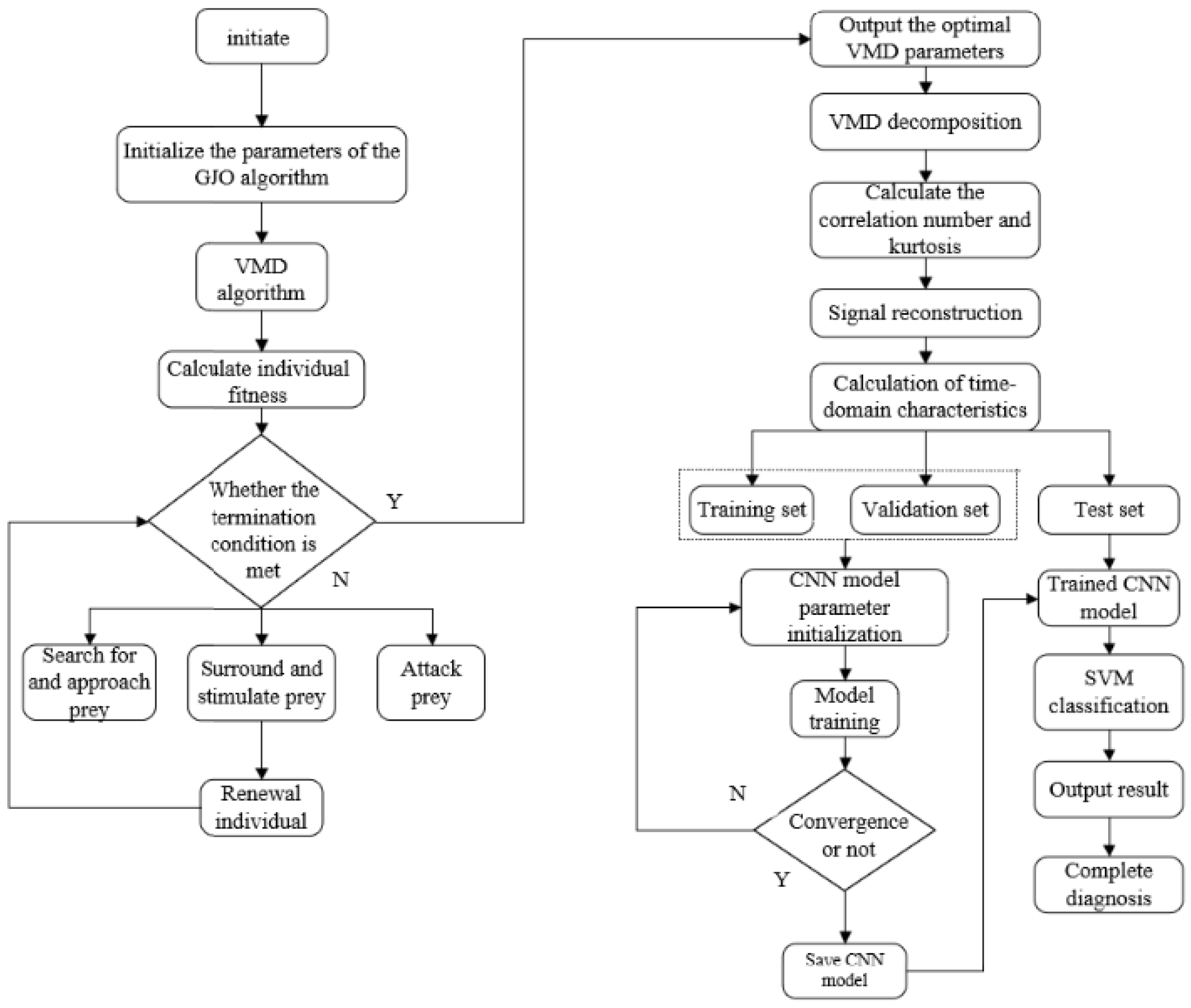
The GJO optimization VMD flowchart is shown in Figure 1.

2.4. Kurtosis Criterion and Cross-Correlation Coefficient Criterion

2.4.1. Kurtosis Criterion

Kurtosis is a dimensionless parameter which can be defined as
K = E ( x μ ) 4 σ 4
where µ is the mean and standard deviation of x and E(t) is the expectation of t.
The normal bearing vibration signal when working has a crag value of about 3, which approximately obeys the normal distribution, but when the bearing is faulty, the crag value of its fault signal will increase [28].

2.4.2. Cross-Correlation Coefficient Criterion

In this paper, the joint crag and the number of interrelationships criteria are reconstructed by taking the components that satisfy both the crag and the number of interrelationships criteria in order to achieve noise reduction in actual bearing fault diagnosis.

2.5. Time-Domain Indicators

In this paper, we construct the feature matrix by calculating the time-domain metrics of the signal reconstructed by VMD decomposition, including the mean, variance, peak, crag, RMS, etc. Nine indicators [29] are used as inputs for the deep learning network to provide more meaningful and interpretable data. This aids the neural network in learning more effectively, leading to improved model accuracy and robustness.

2.6. CNN-SVM Combined Network Architecture

The CNN-SVM network combination is made by using SVM as a classifier instead of the original output layer in the convolutional neural network. The powerful multi-classification ability of the SVM is utilized to improve the classification ability of the normal CNN network in order to improve the performance of the whole network. Figure 2 shows the structure of the CNN-SVM. The process is as follows: the data are first fed into the input layer of the network, and then the CNN is trained until the training process converges so that useful features can be extracted. Then, the features are input into the SVM for classification, thus fully utilizing the advantages of both.

2.7. Diagnostic Process

Based on the above theory, this paper introduces a fault diagnosis method combining time-domain features with GJO-VMD and the CNN-SVM. The process is as follows:
(1)
The original data are subjected to data partitioning, the partitioned data are fed into the GJO algorithm, the fitness function of the algorithm is set as well as the various parameters, and the optimal parameters, k and α, that are most suitable for the VMD decomposition of each signal are determined based on the different characteristics of the different data.
(2)
The best parameters obtained are substituted into VMD for signal decomposition to obtain the respective decomposed IMF components.
(3)
The kurtosis value and cross-correlation coefficient value of each IMF component are calculated and the component that meets both the kurtosis criterion and the cross-correlation coefficient criterion for signal reconstruction is selected so as to obtain the signal after noise reduction.
(4)
The mean, variance, peak, magnitude, RMS, peak factor, pulse factor, waveform factor, and margin factor of the reconstructed signal are calculated to form the feature data.
(5)
The composed feature data are used as the input to the CNN-SVM network to realize the bearing fault diagnosis.
The flowchart is shown in Figure 3.

3. Results

3.1. Public Dataset Testing

(1)
Experimental data
The Case Western Reserve University (CWRU) bearing dataset, the authoritative public dataset in the field of bearing fault diagnosis, was used for testing. The model of the bearings used in the experiment is SKF6205, and the sampling frequency is 12 kHz, the rotational speed is 1797 r/min, and the load is 0HP. The data of the inner ring, outer ring, and rolling body failure, as well as normal data under the diameters of 0.1778 mm, 0.3556 mm, and 0.5334 mm are selected for a total of 10 kinds of conditions; 120 groups of samples are taken for each kind of condition, and the length of the sample for each kind of sample is 2048. The experimental platform is Matlab software (The version is R2023) for diagnosis and analysis.
(2)
Construct the feature data vector
The bearing data were processed using GJO-VMD to filter and reconstruct the components containing important fault features and construct the feature data vectors. In the GJO optimization VMD process, the parameters of GJO were set as follows: the population size was 20, the maximum number of iterations was 20, the range of k was 100–2500, the range of α was 3–10, and the number of optimization variables was 2. The results are shown in Table 1.
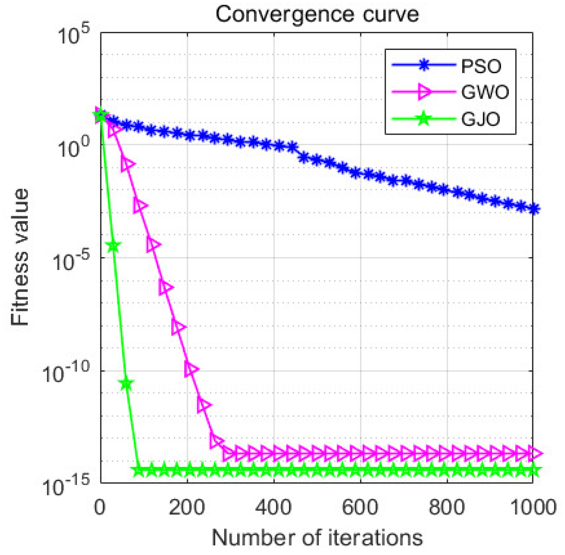
To demonstrate the effectiveness of the GJO algorithm, this paper selects the data of the inner ring fault with a diameter of 0.5334 mm as the comparison data and compares the two algorithms, the GJO algorithm, the GWO algorithm, and the PSO algorithm, obtaining the convergence curves, as shown in Figure 4, which shows the superiority of the GJO algorithm.
The best value (5, 1621) obtained from the optimization is brought to VMD for decomposition, and the obtained time domain and frequency domain diagrams are shown in Figure 5, from which it can be obtained that the five components obtained from the decomposition are uniformly distributed in each frequency from low to high according to the center frequency, that there is no occurrence of modal mixing phenomena existing in the EMD method, and that the GJO-VMD method decomposes the signal with better effect.
To enable the more efficient extraction of fault features from the fault signal, the component signals are screened by calculating the kurtosis value of each component and the cross-correlation coefficient between the component and the original signal.
Based on the fact that the vibration signal of a bearing under normal conditions approximately follows a normal distribution with a kurtosis value around three, when a fault occurs in the bearing, the kurtosis value significantly increases. According to this theory, when the kurtosis value of certain IMF components exceeds three, it indicates that these components contain substantial impact components. This means that a considerable amount of fault-related impact content from the original signal is included in these components. By reconstructing these components, the resulting signal shows a significant increase in kurtosis. The more pronounced the fault, the greater the increase in kurtosis.
The cross-correlation coefficient is defined as the correlation between each IMF component and the original signal. It is determined using the autocorrelation of the original signal, with the magnitude of the correlation coefficient between each component and the original signal serving as the criterion for selecting relevant components. It can be observed that the magnitude of this value is directly proportional to the richness of the fault information represented by the component.
The kurtosis values and cross-correlation coefficient values of the five components obtained from the computational decomposition are presented in Table 2. As can be seen from Table 2, IMF1 and IMF2 are reconstructed as their kurtosis values are greater than three and the cross-correlation coefficient values are greater than the other components. Calculate the time-domain information and generate the feature data, which are used as inputs to the CNN-SVM model to help the model learn better, so as to improve the accuracy and robustness of the model.
(3)
Fault diagnosis
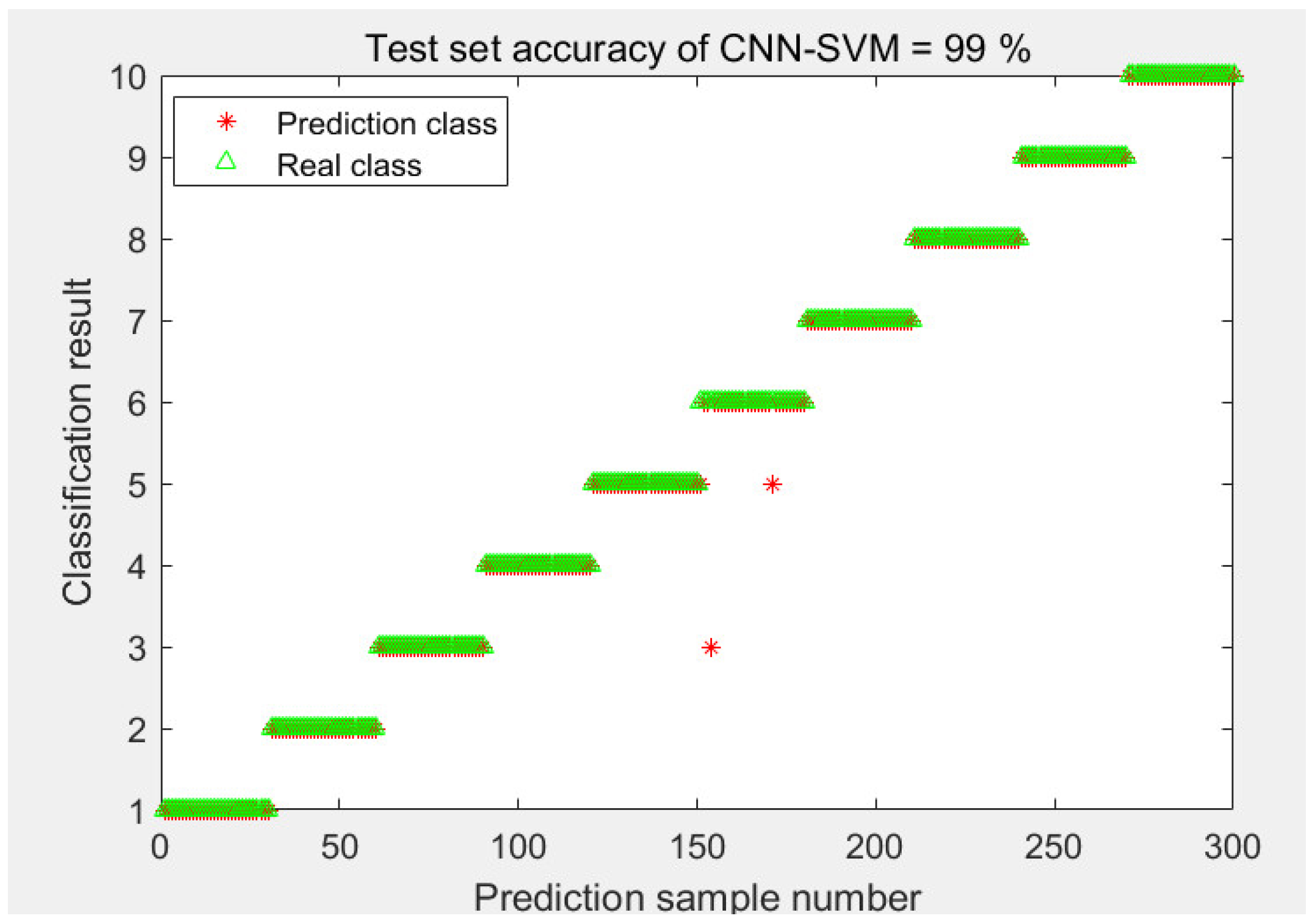
Divide the data into a training set (70%), a verification set (20%), and a test set (10%). The parameters of the model are shown in Table 3. The learning rate of the network was set to 0.01, and the maximum number of iterations was 150, resulting in the confusion matrix of the model, as shown in Figure 6, and the classification outcomes for the test set samples are illustrated in Figure 7. All except categories six achieve 100% accuracy, and the average accuracy also reaches 99%, with a running time of 21.56 s, which is also relatively efficient.
(4)
Model Comparison
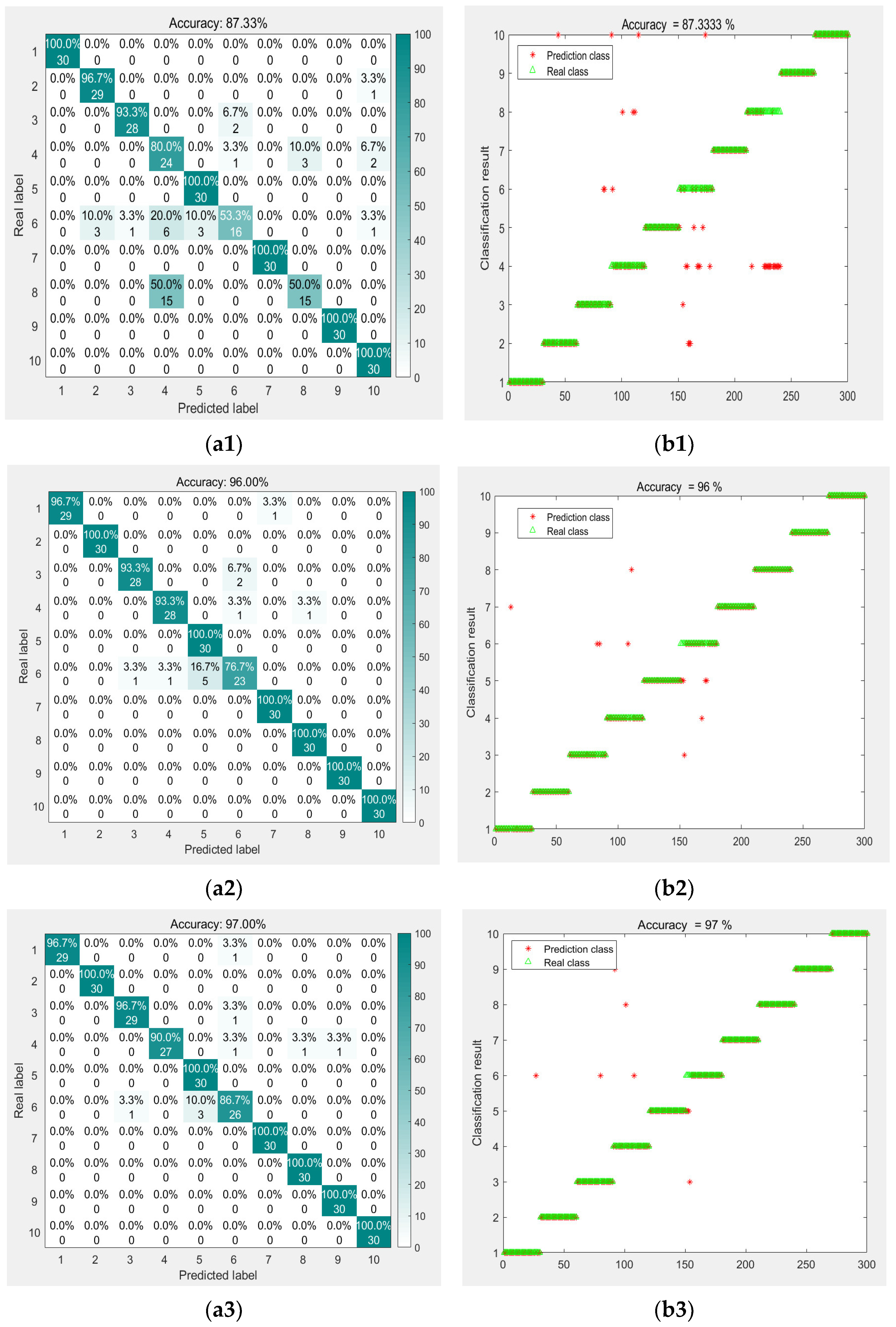
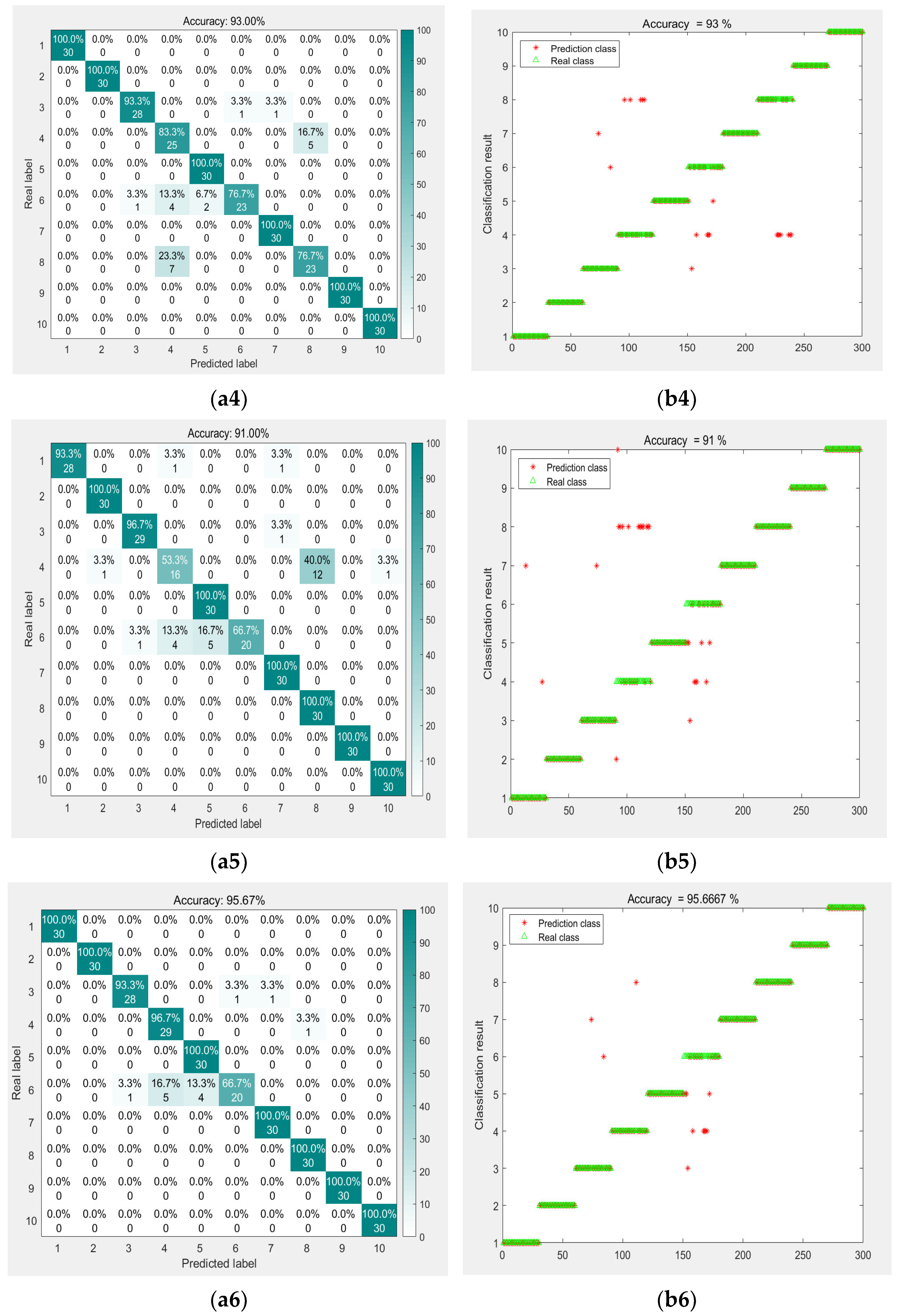
To demonstrate the superiority of the GJO-VMD method combined with the time-domain features and CNN-SVM model, it is compared with the CNN, LSTM, BILSTM, VMD-CNN, VMD-CNN-SVM, and GJO-VMD-CNN-SVM models for comparison, and the parameter settings of the network models are all the same as those presented in this paper. In order to avoid the interference caused by random factors, this paper will perform the training of different models several times to verify the generalization of the model and its robustness. The model comparison is shown in Table 4. The confusion matrix and classification results are shown in Figure 8. The superiority of the model can also be seen in the final results.
From the data in the table, it can be seen that the average accuracy of the GJO-VMD method combined with time-domain features and the CNN-SVM bearing fault diagnosis model proposed in this paper is significantly improved compared to the other models after multiple trainings, and the superiority of the model can also be concluded.

3.2. Experimental Verification

(1)
Experimental data presentation and processing
This paper proposes a model and assesses its feasibility, as can be seen after testing and using the publicly available dataset, which will now be further verified using the experimental data measured by the experimental equipment provided by the Changchun University Mechanical Laboratory (Changchun, China).
The experimental equipment shown in Figure 9 includes bearing type SKF6007 deep groove ball bearings, and the bearing failure types include inner ring failure, outer ring failure, rolling element failure, and a normal state. The motor speed of the experimental bench is set to 2000 r/min, the load is 1000 N, and the sampling frequency is 20 kHz. One hundred and twenty sets of samples are taken for each state, and the sample length of each set of samples is 2048. The optimal parameters corresponding to the VMDs for the four states are optimized using GJO as (5, 715), (3, 885), (4, 925), and (9, 1218), respectively. The obtained optimal parameters are substituted into VMD for decomposition and then reconstructed using the kurtosis and the cross-correlation coefficient; the nine time-domain features of the reconstructed signals are computed once to construct the feature matrix, which is inputted into the CNN-SVM model.
(2)
Analysis of experimental results
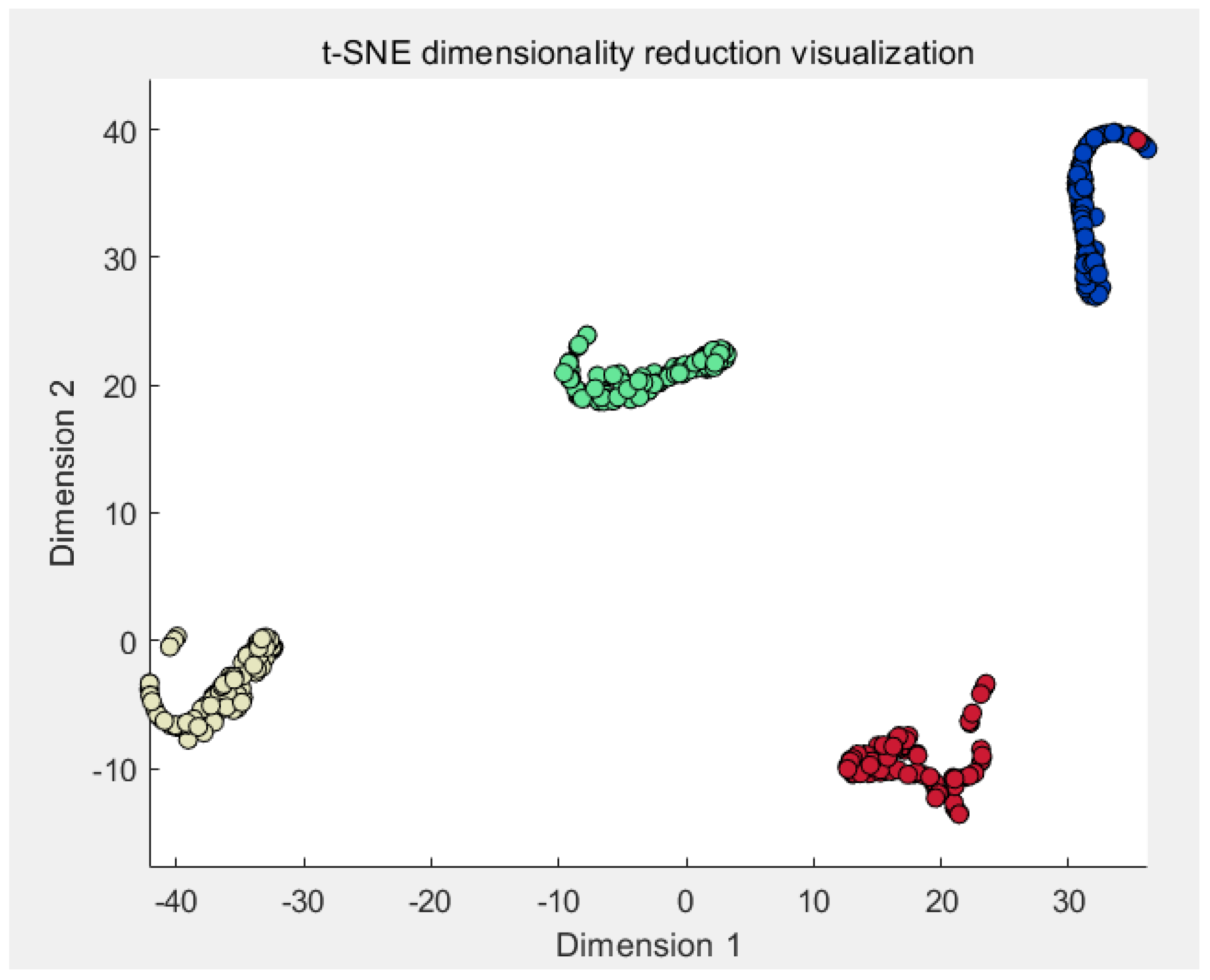
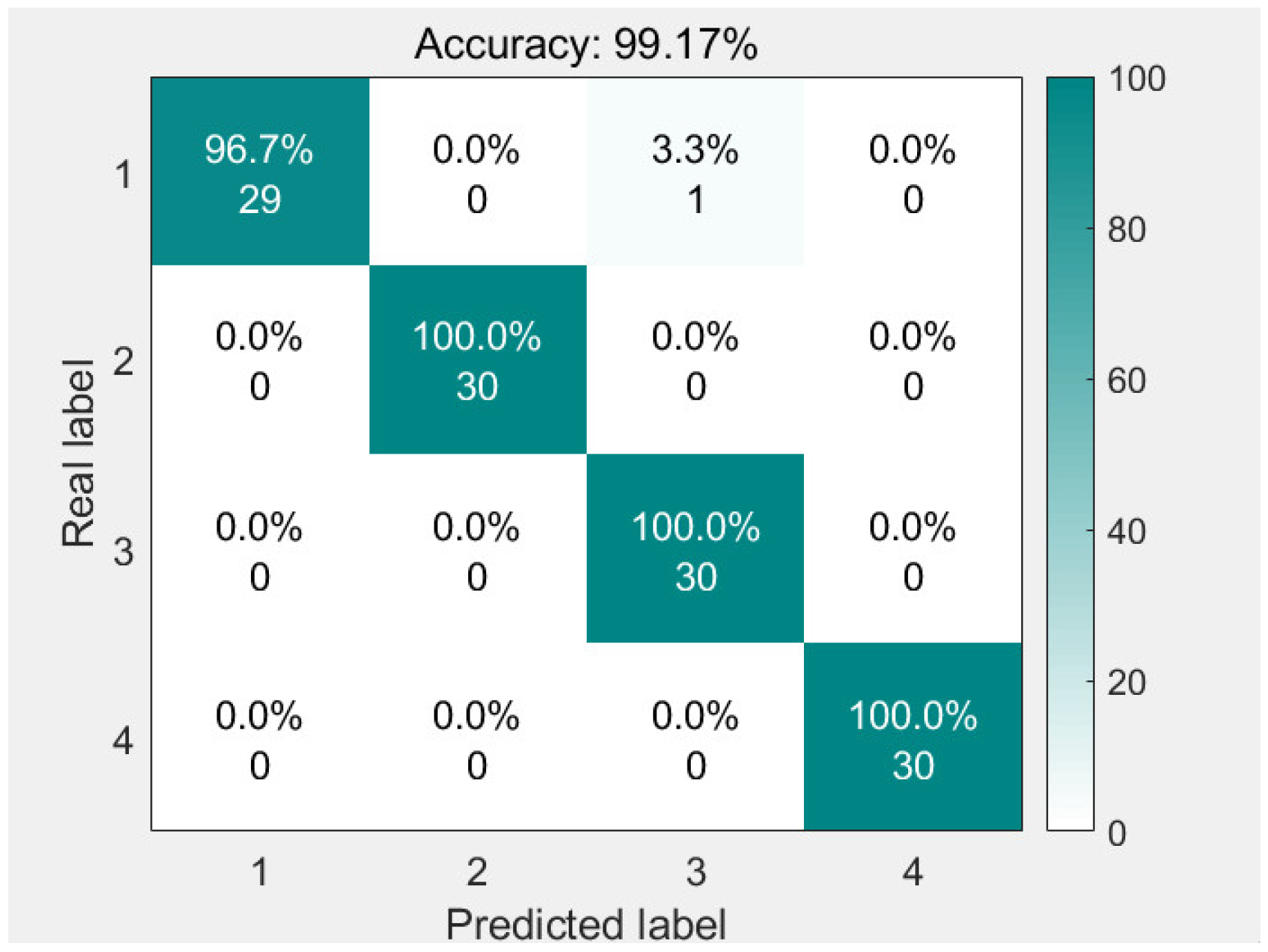
The experimental results are presented using visualization, as shown in Figure 10, the confusion matrix obtained after the model training is completed, as shown in Figure 11, and the classification results are shown in Figure 12. As can be seen in the figure, the model proposed in this paper reaches 99.17% in terms of diagnostic accuracy, and the time was 23 s; the diagnostic efficiency of the model is also fully in line with the application of the requirements of the model. The model not only demonstrates a good performance in the public dataset, but, in the actual experiments, can also provide good diagnostic results, which proves that the model can be completely applied to actual bearing fault diagnosis experiments.
(3)
Model comparison
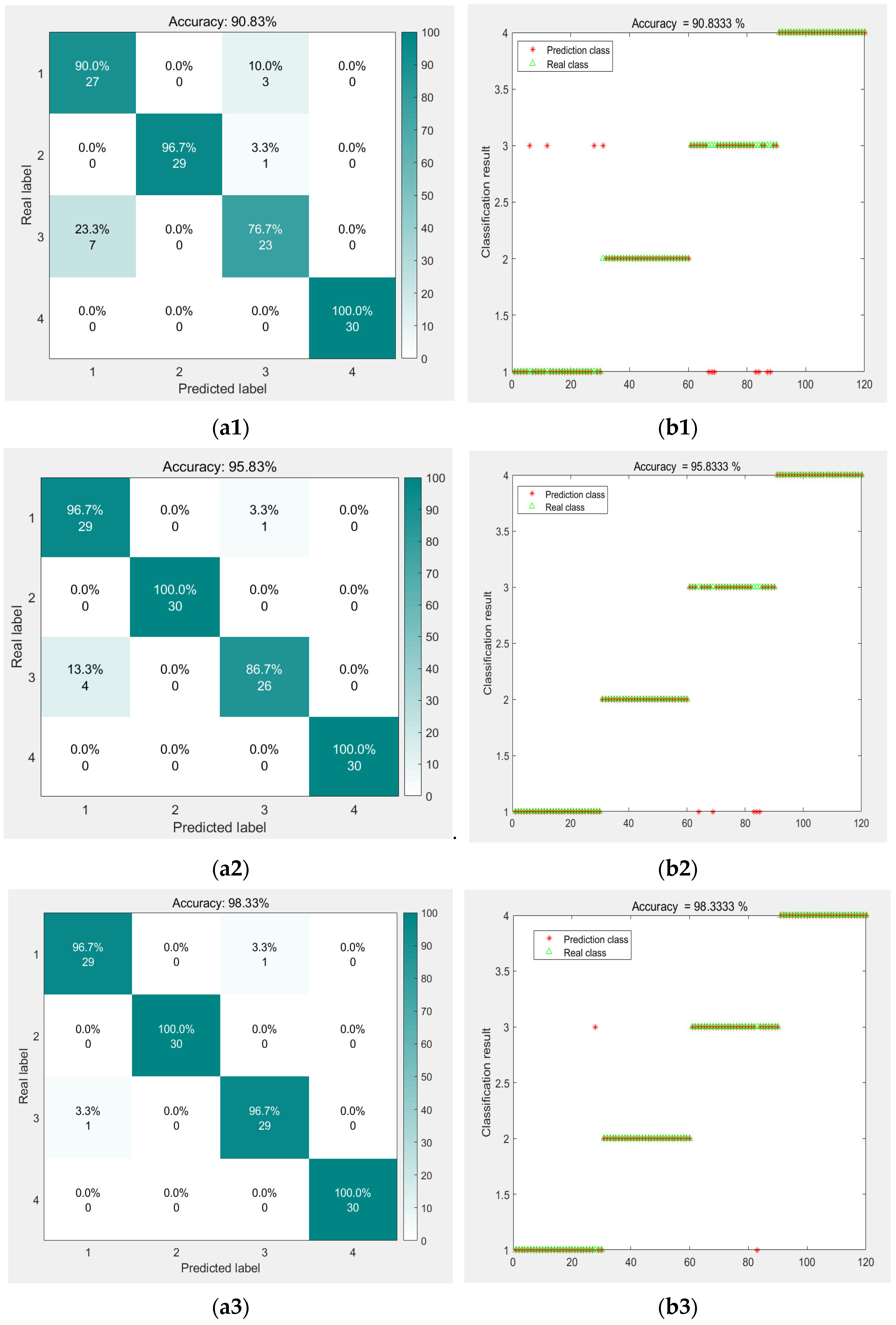
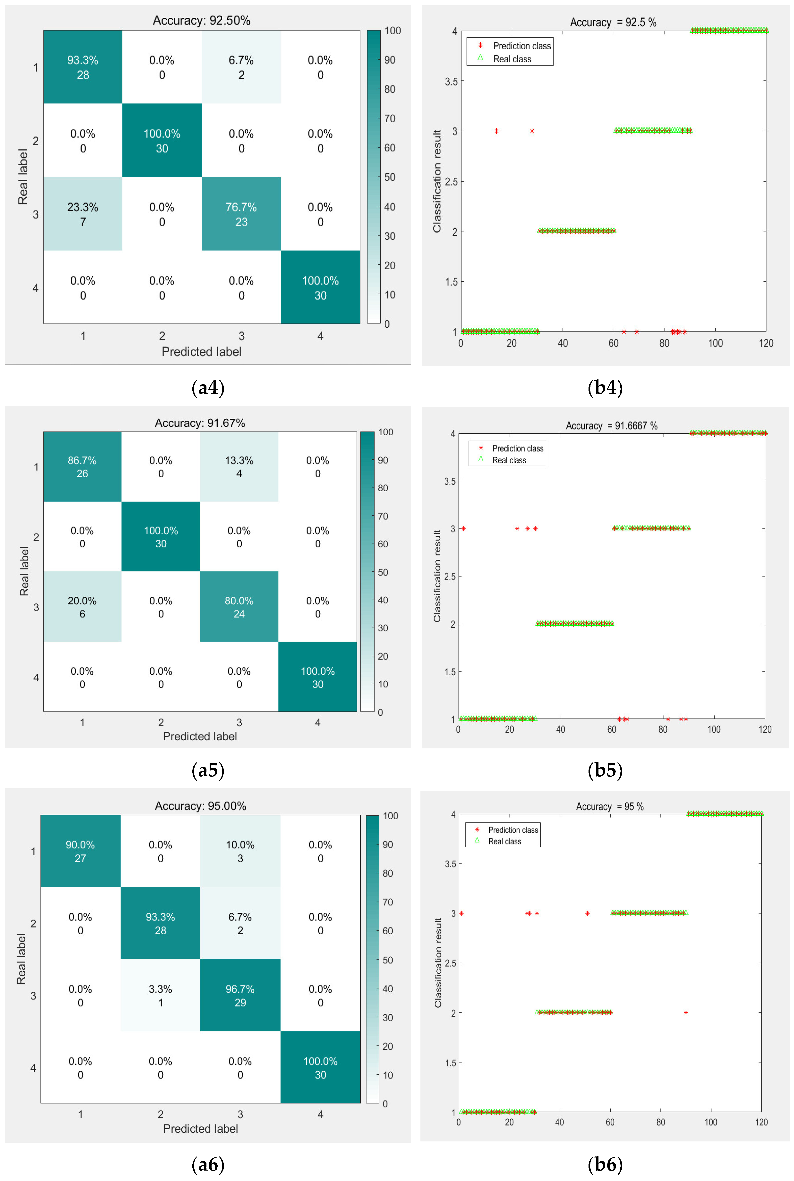
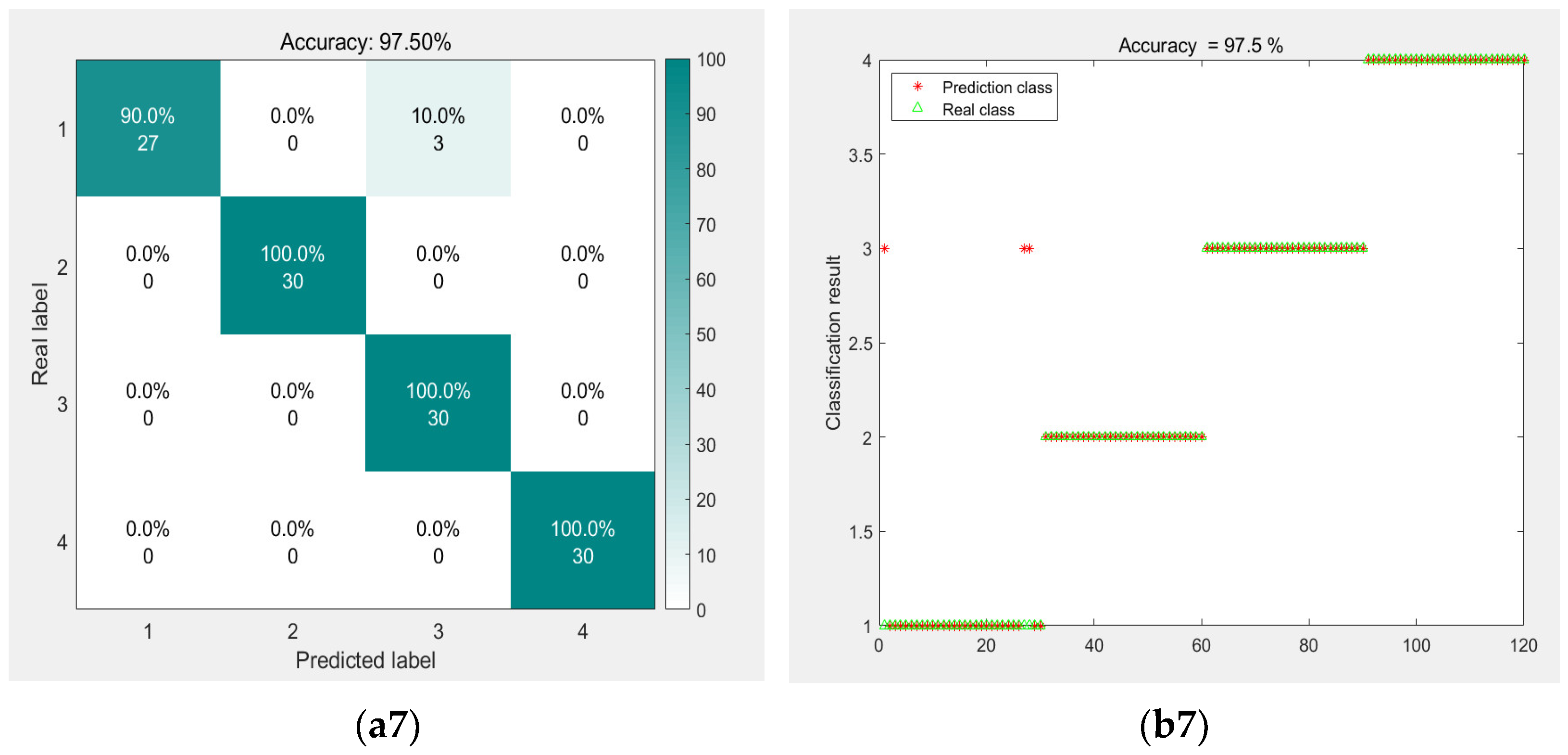
Using these data, the proposed model in this paper is compared again with other models. The model comparisons are shown in Table 5, and the comparison results are illustrated in Figure 13. Observing the results, it is evident that the performance of this model still surpasses that of the other models.
(4)
Noise test
To intuitively validate the feasibility of the model under noisy conditions, additional noise was introduced into the original data to conduct experiments evaluating the model’s feasibility across different noise levels. The signal-to-noise ratio (SNR) is defined as the ratio of the power of the signal (Power of Signal) to the power of the noise (Power of Noise) [30]. The formula is expressed as follows:
S N R = 10 log 10 P s i g n a l P n o i s e
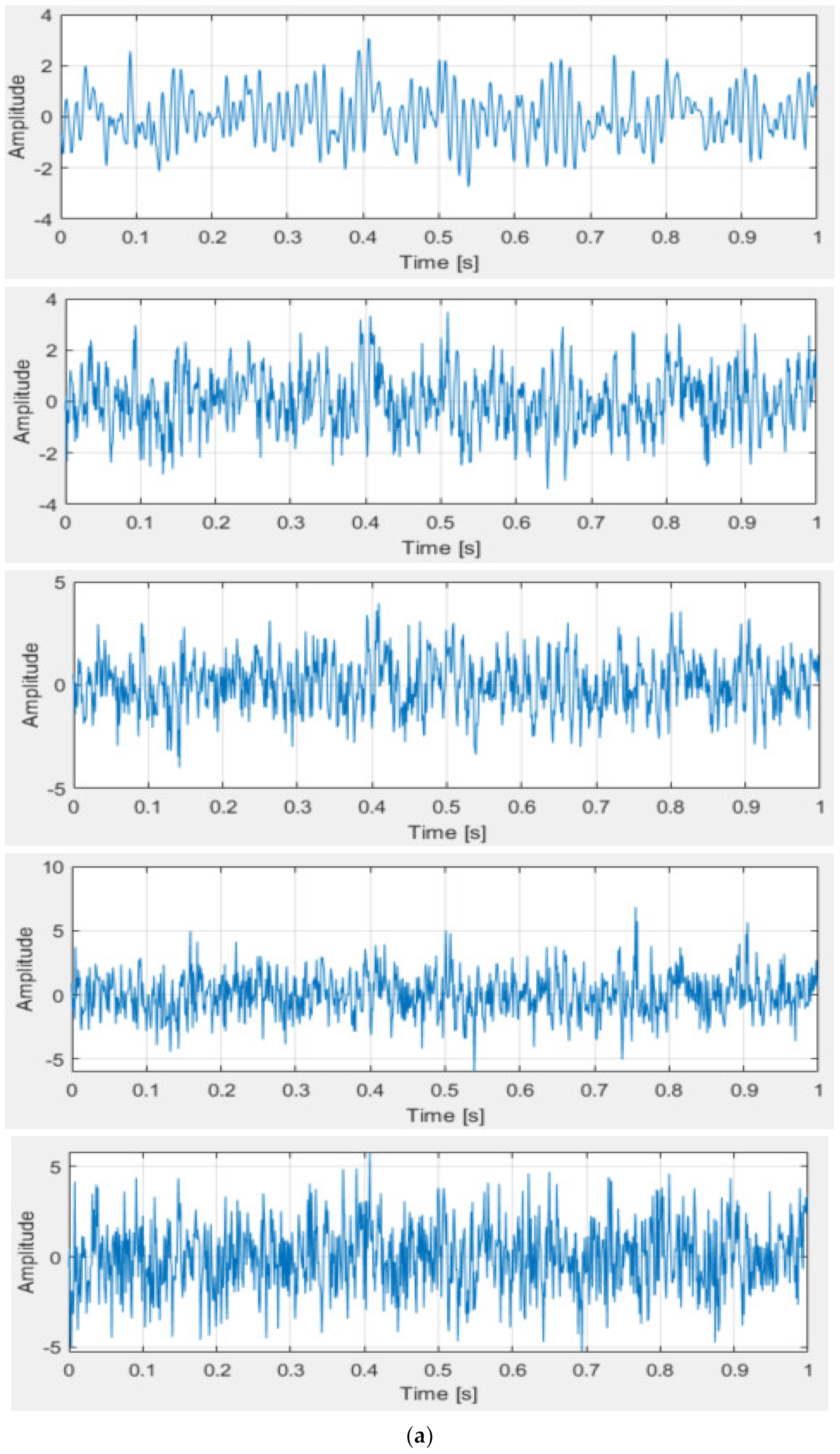
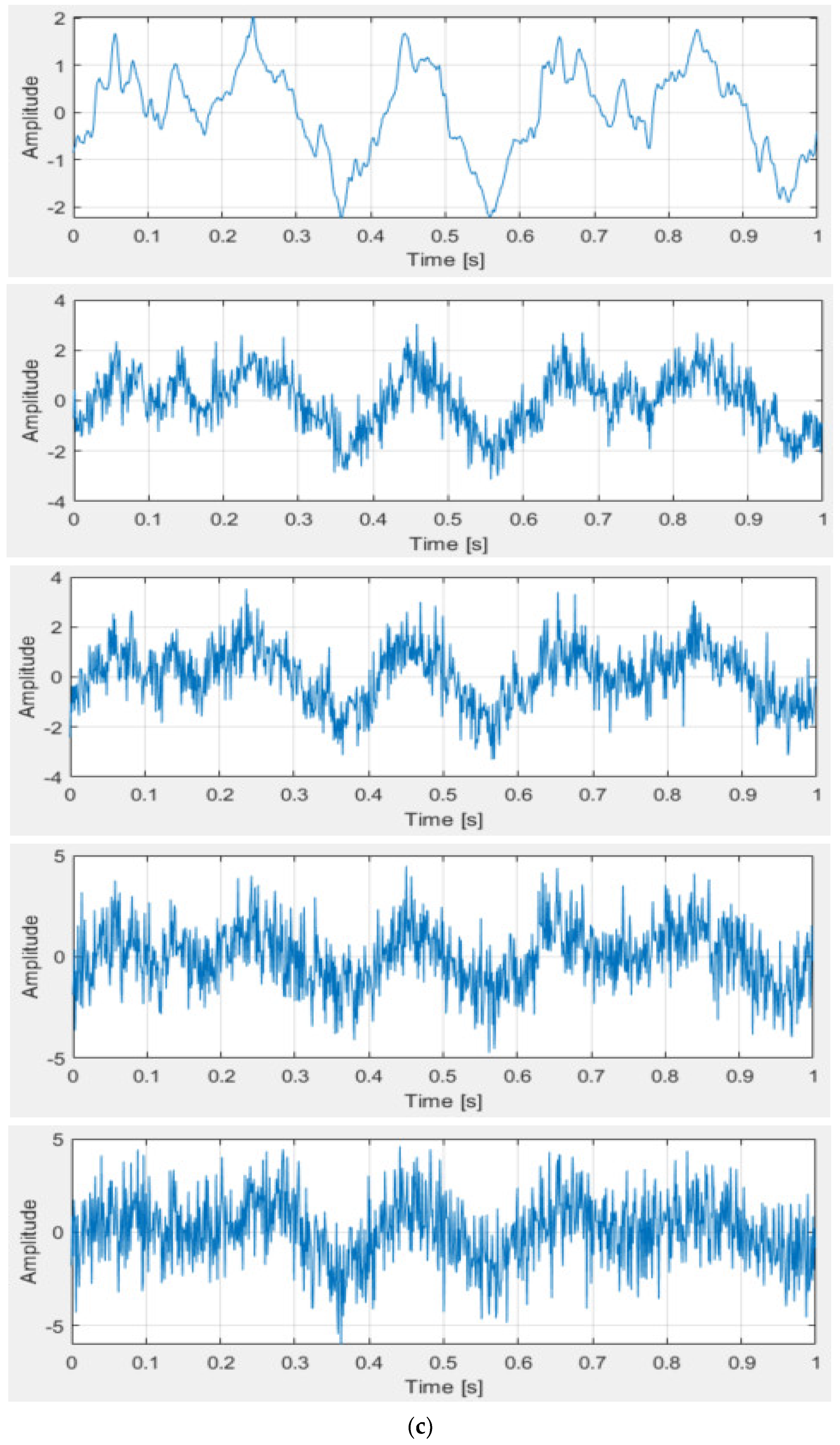
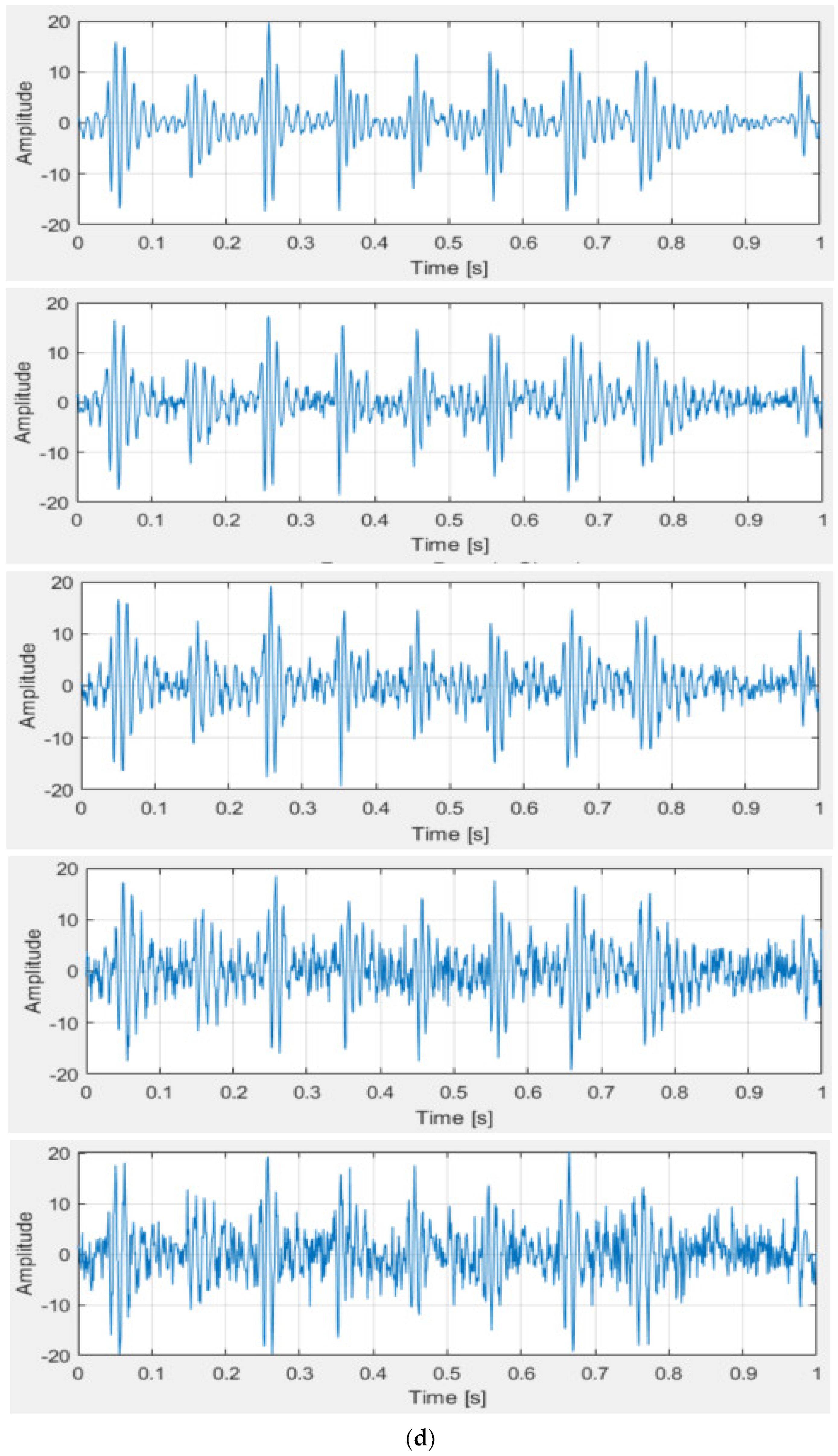
Different values of the SNR represent different conditions. When the SNR is positive, it indicates that the signal strength is greater than the noise strength, simulating an environment with moderate noise. However, when the SNR is negative, it implies that the noise strength exceeds the signal strength, indicating significant signal degradation and simulating a harsher environment. Based on these conclusions, four distinct SNR values of −4, −2, 2, and 4 were added to simulate various environments. The time-domain representations of the original signal and the signals with different SNR levels are shown in Figure 14, ordered from top to bottom as the original signal, SNR = 4, SNR = 2, SNR = −2, and SNR = −4.
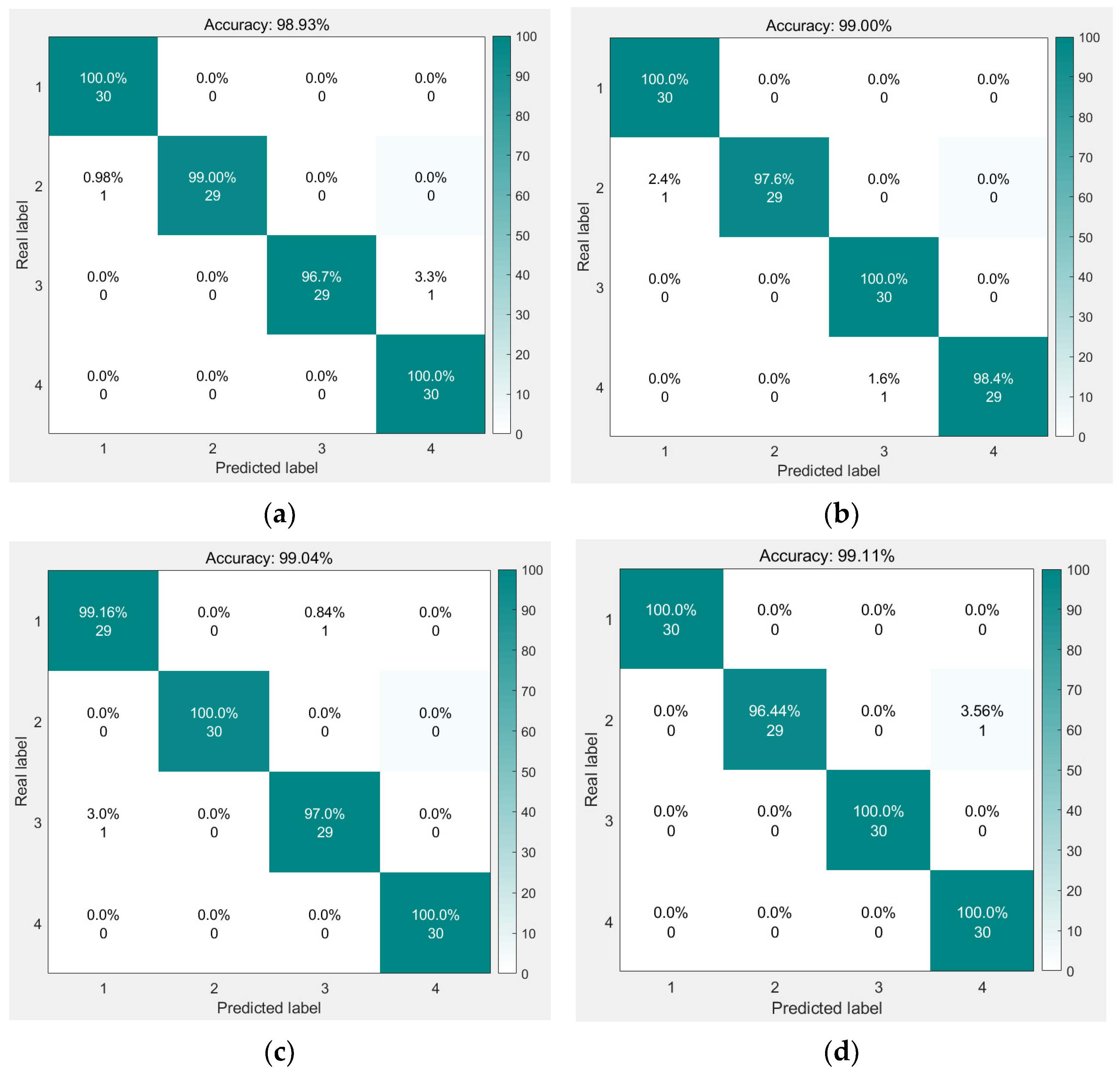
After adding noise with different SNR levels to the original signal, the proposed model was used to perform fault diagnosis for each case. The resulting confusion matrix is shown in Figure 15. The confusion matrix indicates that despite the signal being affected by environmental and machine vibration noise, along with the added white noise, the model still achieved an accuracy of approximately 90%. This demonstrates the model’s feasibility under real-world operating conditions.

4. Discussion

To minimize the impact of noise in fault diagnosis and the consequent problem of the difficulty in extracting the fault features, as well as the issue of the low accuracy of the traditional models, the proposed fault diagnosis method of GJO-VMD combining time-domain features and the CNN-SVM is of great significance in solving the above problems.
(1)
In this paper, GJO is used to optimize VMD in order to select the key parameters, PSO and GWO algorithms are compared, and the results demonstrate that the GJO algorithm converges rapidly and maintains high accuracy.
(2)
The VMD-decomposed signals are filtered and reconstructed using the kurtosis and cross-correlation coefficient, and the nine time-domain features of the reconstructed signals are calculated while simultaneously constructing the feature vectors, which serve as inputs for the neural network so that the neural network can be provided with more meaningful and easy-to-interpret inputs, which then help the model to learn better, thus improving the accuracy and robustness of the model.
(3)
The SVM is utilized to replace the SoftMax classifier in the traditional CNN network to improve the classification ability of the CNN network, which is more conducive to the problems mentioned in this paper.

Author Contributions

Conceptualization, Y.Z. and X.Z.; methodology, Y.Z., X.Z. and W.Z.; software, X.Z.; validation, X.Z., T.L. and W.Z.; formal analysis, X.Z.; investigation, X.Z.; resources, X.Z.; data curation, X.Z. and T.L.; writing—original draft preparation, X.Z.; writing—review and editing, X.Z., W.Z. and T.L.; visualization, X.Z.; supervision, Y.Z.; project administration, Y.Z.; funding acquisition, Y.Z. All authors have read and agreed to the published version of the manuscript.

Funding

This research was funded by the Jilin Provincial Department of Science and Technology, grant number 20230101208JC.

Data Availability Statement

The original contributions presented in the study are included in the article, further inquiries can be directed to the corresponding author.

Conflicts of Interest

The authors declare no conflicts of interest.

References

  1. Fang, Q.; Wu, D. ANS-net: Anti-noise Siamese network for bearing fault diagnosis with a few data. Nonlinear Dyn. 2021, 104, 2497–2514. [Google Scholar] [CrossRef]
  2. Cui, B.; Weng, Y.; Zhang, N. A feature extraction and machine learning framework for bearing fault diagnosis. Renew. Energy 2022, 191, 987–997. [Google Scholar] [CrossRef]
  3. Zhang, X.; Zhao, B.; Lin, Y. Machine learning based bearing fault diagnosis using the case western reserve university data: A review. IEEE Access 2021, 9, 155598–155608. [Google Scholar] [CrossRef]
  4. Han, T.; Zhang, L.; Yin, Z.; Tan, A.C. Rolling bearing fault diagnosis with combined convolutional neural networks and support vector machine. Measurement 2021, 177, 109022. [Google Scholar] [CrossRef]
  5. Rai, A.; Upadhyay, S.H. A review on signal processing techniques utilized in the fault diagnosis of rolling element bearings. Tribol. Int. 2016, 96, 289–306. [Google Scholar] [CrossRef]
  6. Xu, Y.; Li, Z.; Wang, S.; Li, W.; Sarkodie-Gyan, T.; Feng, S. A hybrid deep-learning model for fault diagnosis of rolling bearings. Measurement 2021, 169, 108502. [Google Scholar] [CrossRef]
  7. Khorram, A.; Khalooei, M.; Rezghi, M. End-to-end CNN+ LSTM deep learning approach for bearing fault diagnosis. Appl. Intell. 2021, 51, 736–751. [Google Scholar] [CrossRef]
  8. Quendo, C.; Rius, E.; Person, C.; Michel, N. Integration of optimized low-pass filters in a bandpass filter for out-of-band improvement. IEEE Trans. Microw. Theory Tech. 2001, 49, 2376–2383. [Google Scholar] [CrossRef]
  9. Zhang, Y.; Yong, L.; Mao, G. Complementary ensemble adaptive local iterative filtering and its application to rolling bearing fault diagnosis. IEEE Access 2021, 9, 47275–47293. [Google Scholar] [CrossRef]
  10. Zhang, T.; Liu, S.; Wei, Y.; Zhang, H. A novel feature adaptive extraction method based on deep learning for bearing fault diagnosis. Measurement 2021, 185, 110030. [Google Scholar] [CrossRef]
  11. Huang, N.E.; Shen, Z.; Long, S.R.; Wu, M.C.; Shih, H.H.; Zheng, Q.; Yen, N.-C.; Tung, C.C.; Liu, H.H. The empirical mode decomposition and the Hilbert spectrum for nonlinear and non-stationary time series analysis. Proc. R. Soc. Lond. Ser. A Math. Phys. Eng. Sci. 1998, 454, 903–995. [Google Scholar] [CrossRef]
  12. Wu, Z.; Huang, N.E. Ensemble empirical mode decomposition: A noise-assisted data analysis method. Adv. Adapt. Data Anal. 2009, 1, 1–41. [Google Scholar] [CrossRef]
  13. Yeh, J.R.; Shieh, J.S.; Huang, N.E. Complementary ensemble empirical mode decomposition: A novel noise enhanced data analysis method. Adv. Adapt. Data Anal. 2010, 2, 135–156. [Google Scholar] [CrossRef]
  14. Torres, M.E.; Colominas, M.A.; Schlotthauer, G.; Flandrin, P.A. A complete ensemble empirical mode decomposition with adaptive noise. In Proceedings of the 2011 IEEE International Conference on Acoustics, Speech and Signal Processing (ICASSP), Prague, Czech Republic, 22–27 May 2011; IEEE: Piscataway, NJ, USA; pp. 4144–4147. [Google Scholar]
  15. Duan, R.; Liao, Y.; Wang, S. Adaptive morphological analysis method and its application for bearing fault diagnosis. IEEE Trans. Instrum. Meas. 2021, 70, 1–10. [Google Scholar] [CrossRef]
  16. Dragomiretskiy, K.; Zosso, D. Variational mode decomposition. IEEE Trans. Signal Process. 2013, 62, 531–544. [Google Scholar] [CrossRef]
  17. Li, Y.; Cheng, G.; Liu, C. Research on bearing fault diagnosis based on spectrum characteristics under strong noise interference. Meas. 2021, 169, 108509. [Google Scholar] [CrossRef]
  18. Ye, M.; Yan, X.; Jia, M. Rolling bearing fault diagnosis based on VMD-MPE and PSO-SVM. Entropy 2021, 23, 762. [Google Scholar] [CrossRef]
  19. Zhang, P.; Zhang, W.; Zhao, X.; Wu, X.; Liu, N. Application of WOA-VMD algorithm in bearing fault diagnosis. Noise Vib. Control 2021, 41, 86. [Google Scholar]
  20. Wang, M.; Wang, W.; Zeng, J.; Zhang, Y. An integrated method based on sparrow search algorithm improved variational mode decomposition and support vector machine for fault diagnosis of rolling bearing. J. Vib. Eng. Technol. 2022, 10, 2893–2904. [Google Scholar] [CrossRef]
  21. Li, H.; Liu, T.; Wu, X.; Chen, Q. An optimized VMD method and its applications in bearing fault diagnosis. Measurement 2020, 166, 108185. [Google Scholar] [CrossRef]
  22. Antoni, J. The spectral kurtosis: A useful tool for characterising non-stationary signals. Mech. Syst. Signal Process. 2006, 20, 282–307. [Google Scholar] [CrossRef]
  23. Nayana, B.R.; Geethanjali, P. Analysis of statistical time-domain features effectiveness in identification of bearing faults from vibration signal. IEEE Sens. J. 2017, 17, 5618–5625. [Google Scholar] [CrossRef]
  24. Sawalhi, N.; Randall, R.B. The application of spectral kurtosis to bearing diagnostics. In Proceedings of the ACOUSTICS 2004, Gold Coast, Australia, 3–5 November 2004; pp. 3–5. [Google Scholar]
  25. Liu, X.; Sun, W.; Li, H.; Hussain, Z.; Liu, A. The method of rolling bearing fault diagnosis based on multi-domain supervised learning of convolution neural network. Energies 2022, 15, 4614. [Google Scholar] [CrossRef]
  26. You, K.; Qiu, G.; Gu, Y. Rolling bearing fault diagnosis using hybrid neural network with principal component analysis. Sensors 2022, 22, 8906. [Google Scholar] [CrossRef]
  27. Chopra, N.; Ansari, M. Golden jackal optimization: A novel nature-inspired optimizer for engineering applications. Expert Syst. Appl. 2022, 198, 116924. [Google Scholar] [CrossRef]
  28. Wang, H.; Liu, Z.; Peng, D.; Cheng, Z. Attention-guided joint learning CNN with noise robustness for bearing fault diagnosis and vibration signal denoising. ISA Trans. 2022, 128, 470–484. [Google Scholar] [CrossRef]
  29. Jiang, Z.; Li, Y.; Gao, J.; Wu, C. A fault detection of aero-engine rolling bearings based on CNN-BiLSTM network integrated cross-attention. Meas. Sci. Technol. 2024, 35, 126116. [Google Scholar] [CrossRef]
  30. Wang, Y.; Huang, S.; Dai, J.; Tang, J. A Novel Bearing Fault Diagnosis Methodology Based on SVD and One-Dimensional Convolutional Neural Network. Shock. Vib. 2020, 2020, 1850286. [Google Scholar] [CrossRef]
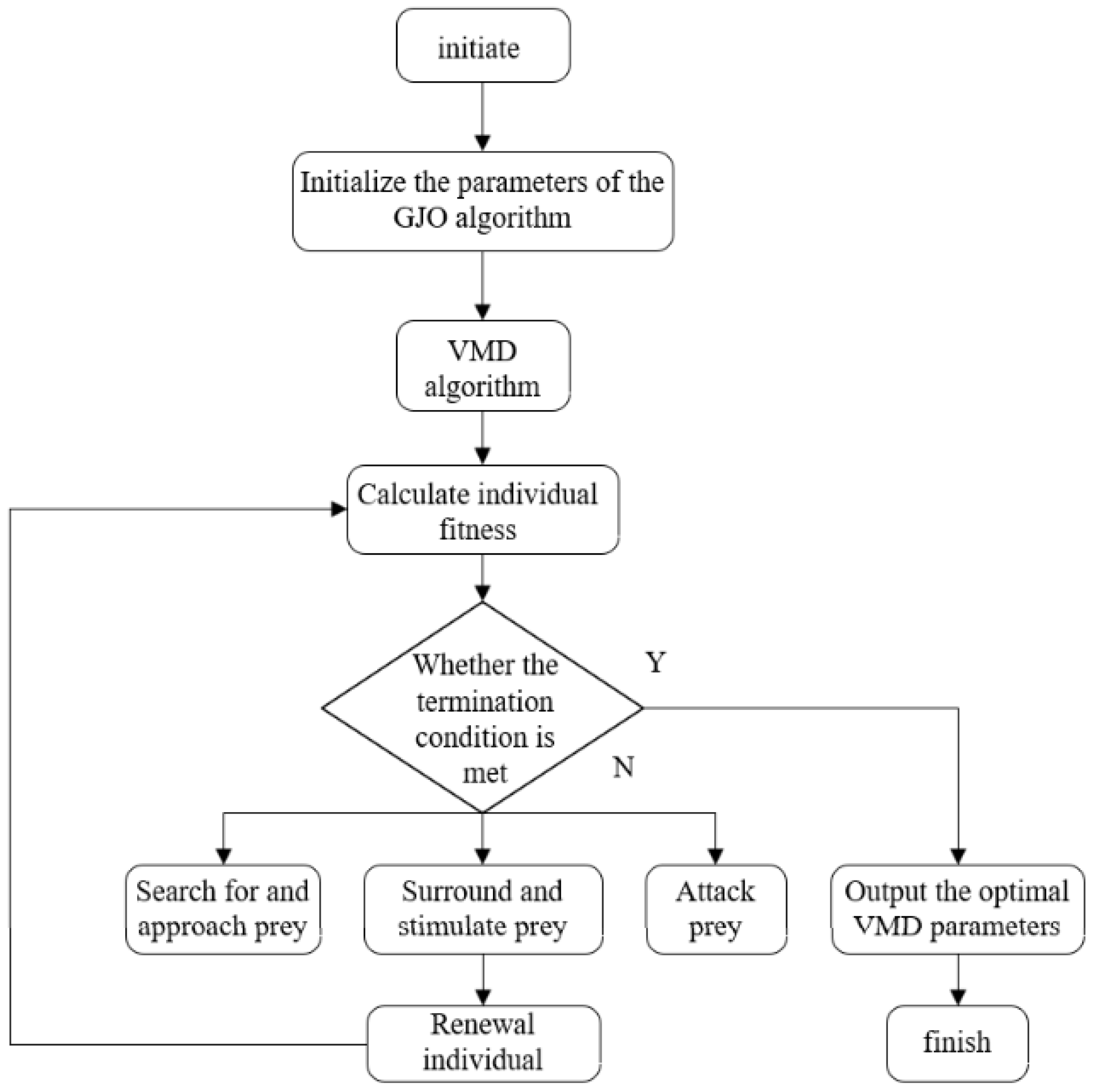
Figure 1. Flowchart of GJO-optimized VMD.
Wevj 15 00544 g001
Figure 2. CNN-SVM structure diagram.
Wevj 15 00544 g002
Figure 3. Diagnostic flowchart.
Wevj 15 00544 g003
Figure 4. Comparison of algorithms.
Wevj 15 00544 g004
Figure 5. (a) Time domain diagram. (b) Frequency domain plot.
Wevj 15 00544 g005
Figure 6. Confusion matrix.
Wevj 15 00544 g006
Figure 7. Sample classification results.
Wevj 15 00544 g007
Figure 8. (a1) CNN. (b1) CNN. (a2) LSTM. (b2) LSTM. (a3) BILSTM. (b3) BILSTM. (a4) CNN-SVM. (b4) CNN-SVM. (a5) VMD-CNN. (b5) VMD-CNN. (a6) VMD-CNN-SVM. (b6) VMD-CNN-SVM. (a7) GJO-VMD-CNN-SVM. (b7) GJO-VMD-CNN-SVM.
Wevj 15 00544 g008aWevj 15 00544 g008bWevj 15 00544 g008c
Figure 9. Diagram of experimental equipment.
Wevj 15 00544 g009
Figure 10. Visualization of training results.
Wevj 15 00544 g010
Figure 11. Confusion matrix.
Wevj 15 00544 g011
Figure 12. Sample classification results.
Wevj 15 00544 g012
Figure 13. (a1) CNN. (b1) CNN. (a2) LSTM. (b2) LSTM. (a3) BILSTM. (b3) BILSTM. (a4) CNN-SVM. (b4) CNN-SVM. (a5) VMD-CNN. (b5) VMD-CNN. (a6) VMD-CNN-SVM. (b6) VMD-CNN-SVM. (a7) GJO-VMD-CNN-SVM. (b7) GJO-VMD-CNN-SVM.
Wevj 15 00544 g013aWevj 15 00544 g013bWevj 15 00544 g013c
Figure 14. (a) The time-domain waveform of the bearing under normal conditions. (b) The time-domain waveform of the bearing in an inner race fault condition. (c) The time-domain waveform of the bearing in an outer race fault condition. (d) The time-domain waveform of the bearing in a rolling element fault condition.
Wevj 15 00544 g014aWevj 15 00544 g014bWevj 15 00544 g014cWevj 15 00544 g014d
Figure 15. (a) The confusion matrix for SNR = −4. (b) The confusion matrix for SNR = −2. (c) The confusion matrix for SNR = 2. (d) The confusion matrix for SNR = 4.
Wevj 15 00544 g015
Table 1. Optimal parameters for VMD.
Fault DiameterTypology(k, α)
0Normal(10, 1847)
0.1778 mmInner ring failure(3, 2500)
0.1778 mmRolling body failure(10, 754)
0.1778 mmOuter ring failure(4, 100)
0.3556 mmInner ring failure(4, 2304)
0.3556 mmRolling body failure(10, 1213)
0.3556 mmOuter ring failure(10, 2352)
0.5334 mmInner ring failure(5, 1621)
0.5334 mmRolling body failure(3, 2099)
0.5334 mmOuter ring failure(7, 196)
Table 2. Kurtosis and cross-correlation coefficient.
ComponentSteepnessCorrelation Number
IMF14.25140.7536
IMF23.58460.4531
IMF32.45610.2847
IMF42.76150.2354
IMF52.65130.2411
Table 3. Model structural parameters.
Network LayerParameter Setting
Convolutional layer 116@3X1, Step 1
Pooling layer 13X1, Step 2
Convolutional layer 232@2X1, Step 1
Pooling layer 22X1, Step 2
Convolutional layer 364@2X1, Step 1
Pooling layer 32X1, Step 2
Flatten-
SVM-
Table 4. Comparison of model accuracy.
ModelPrecision/%Recall/%F1-ScoreAverage Accuracy/%
CNN89870.8787.33
LSTM96960.9696.00
BILSTM97970.9797.00
CNN-SVM93930.9393.00
VMD—CNN91910.9191.00
VMD—CNN—SVM95950.9495.67
GJO—VMD—CNN—SVM96960.9596.67
GJO-VMD combining time domain features and CNN-SVM99990.9999.05
Table 5. Comparison of model accuracy.
ModelPrecision/%Recall/%F1-ScoreAverage Accuracy/%
CNN91910.9190.83
LSTM96960.9595.83
BILSTM98980.9898.33
CNN-SVM93930.9292.50
VMD—CNN92920.9291.67
VMD—CNN—SVM95950.9595.00
GJO—VMD—CNN—SVM98980.9797.50
GJO-VMD combining time domain features and CNN-SVM99990.9999.17
Disclaimer/Publisher’s Note: The statements, opinions and data contained in all publications are solely those of the individual author(s) and contributor(s) and not of MDPI and/or the editor(s). MDPI and/or the editor(s) disclaim responsibility for any injury to people or property resulting from any ideas, methods, instructions or products referred to in the content.