Research on Optimization of Intelligent Driving Vehicle Path Tracking Control Strategy Based on Backpropagation Neural Network

Abstract

To enhance path tracking precision in intelligent vehicles, this study proposes a lateral–longitudinal control strategy optimized with a Backpropagation (BP) neural network. The strategy employs the BP neural network to dynamically adjust prediction and control time-domain parameters within an established Model Predictive Control (MPC) framework, effectively computing real-time front-wheel steering angles for lateral control. Simultaneously, it integrates an incremental Proportional–Integral–Derivative (PID) approach with a meticulously designed acceleration–deceleration strategy for accurate and stable longitudinal speed tracking. The strategy’s efficiency and superior performance are validated through a comprehensive CarSim(2020)/Simulink(2020b) simulation, demonstrating that the proposed controller adeptly modulates control parameters to adapt to various road adhesion coefficients and vehicle speeds. This adaptability significantly improves tracking and driving dynamics, thereby enhancing accuracy, safety, stability, and real-time responsiveness in the intelligent vehicle tracking control system.

1. Introduction

To reduce the complexity of driving and enhance vehicular safety, autonomous driving technology has gained significant attention for its potential to substantially lower traffic accidents attributed to driver factors. This technology encompasses three main components: environmental perception, decision-making and planning, and motion control, with the latter being a crucial aspect. The primary task of motion control is to follow the planned path output by the decision-making layer, controlling the autonomous vehicle to execute driving, braking, and steering actions to accurately track the reference path [1]. Currently, motion control algorithms can be categorized into three types: geometric-based control methods, non-predictive feedback control, and predictive feedback control.

Geometric-based control methods include pure pursuit control [2] and the Stanley tracking algorithm [3]. Lal et al. [4] designed a lateral control method for intelligent vehicles based on the pure pursuit algorithm, which was validated across various curvatures for path tracking problems. However, in more complex driving environments, this method fails to meet control precision requirements. Yu et al. [5] improved upon this by adaptively adjusting the lookahead distance to enhance tracking, but this approach does not adhere to the systematic parameter adjustment methods of control theory, making it difficult to balance stability and tracking accuracy; non-predictive feedback control algorithms include Proportional–Integral–Derivative (PID) control [6] and sliding mode control [7]. Han et al. [8] transformed the lateral path tracking problem into a heading angle prediction problem and designed a neural network-based adaptive PID lateral tracking controller. Wang et al. [9] targeted the vehicle’s relative speed error as the control objective for longitudinal speed, employing a Radical Basis Function (RBF) neural network-based sliding mode control strategy. While PID and sliding mode control have improved tracking accuracy in complex environments, their lack of future state prediction and external disturbance identification renders them unsatisfactory in high-frequency and highly perturbed environments; predictive feedback control methods include Linear Quadratic Regulator (LQR) control [10] and model predictive control (MPC) [11]. The LQR predictive control algorithm is favored in the industry for its straightforward design and superior performance. However, the effectiveness of LQR controllers decreases significantly in the presence of modeling errors and external disturbances [12]. Compared to LQR, MPC performs rolling optimization within a finite time domain, is suitable for optimization problems under multiple constraints, and considers future driving conditions, making it more effective in curve tracking. However, the computational demand of the MPC algorithm, along with the extensive parameters required to be set, often empirically, poses limitations in practical applications [13,14].

The research mentioned above offers a range of strategies for path tracking control, effectively solving the problem of trajectory tracking in nonlinear systems amid changes in system states. However, for variable-speed intelligent vehicles, the computation time required by optimization algorithms presents a significant challenge for real-time operations. To surmount these hurdles, numerous studies have pivoted towards model predictive control (MPC) methodologies. Kouvaritakis et al. [15] provided a thorough overview of the principles of MPC and its application across various industrial settings, underscoring its strengths in managing multivariable control issues and constraints. Specifically, within autonomous driving systems, MPC can take into account the vehicle’s dynamic model and upcoming environmental information, thereby furnishing more accurate and dependable control strategies. Despite MPC’s demonstrated robust control capabilities, its high computational complexity still poses a challenge for real-time application. To tackle this issue, some research has suggested the use of machine learning techniques to optimize parameter selection and computation processes within MPC. For instance, Sun et al. [16] have significantly enhanced the computational efficiency of the algorithm, while maintaining control performance, by integrating deep learning models to predict key parameters within MPC. Building upon the aforementioned research, an optimization method for an autonomous vehicle path tracking control strategy based on BP neural networks is proposed, which adaptively selects the timing parameters in the MPC control model. This method effectively addresses the issues of low tracking accuracy and poor real-time performance inherent in traditional MPC control models. The strategy has been tested in the simulated environments of dry asphalt, wet rain, and muddy snow, with the primary contents of this research being as follows:

(1) Construct a lateral tracking strategy: Utilizing the established vehicle single-track dynamics model and the model predictive control (MPC) algorithm, employ a Backpropagation (BP) neural network to dynamically select predictive and control time-domain parameters in the control strategy based on varying road adhesion coefficients and vehicle speed conditions. Real-time optimization is used to solve for the front-wheel steering angle control quantity, thereby addressing the lateral control issue.

(2) Develop a longitudinal speed tracking strategy: Building upon the incremental PID longitudinal speed tracking controller, establish a rational acceleration–deceleration switching strategy to prevent damage to the executing mechanism due to frequent acceleration–deceleration switches, thereby enhancing the stability of the speed tracking system.

(3) Establish a co-simulation platform using MATLAB and vehiclesim: Under various experimental conditions in typical straight-line driving and lane-changing scenarios, validate the improved tracking control strategy’s stability, accuracy, and robustness in path tracking.

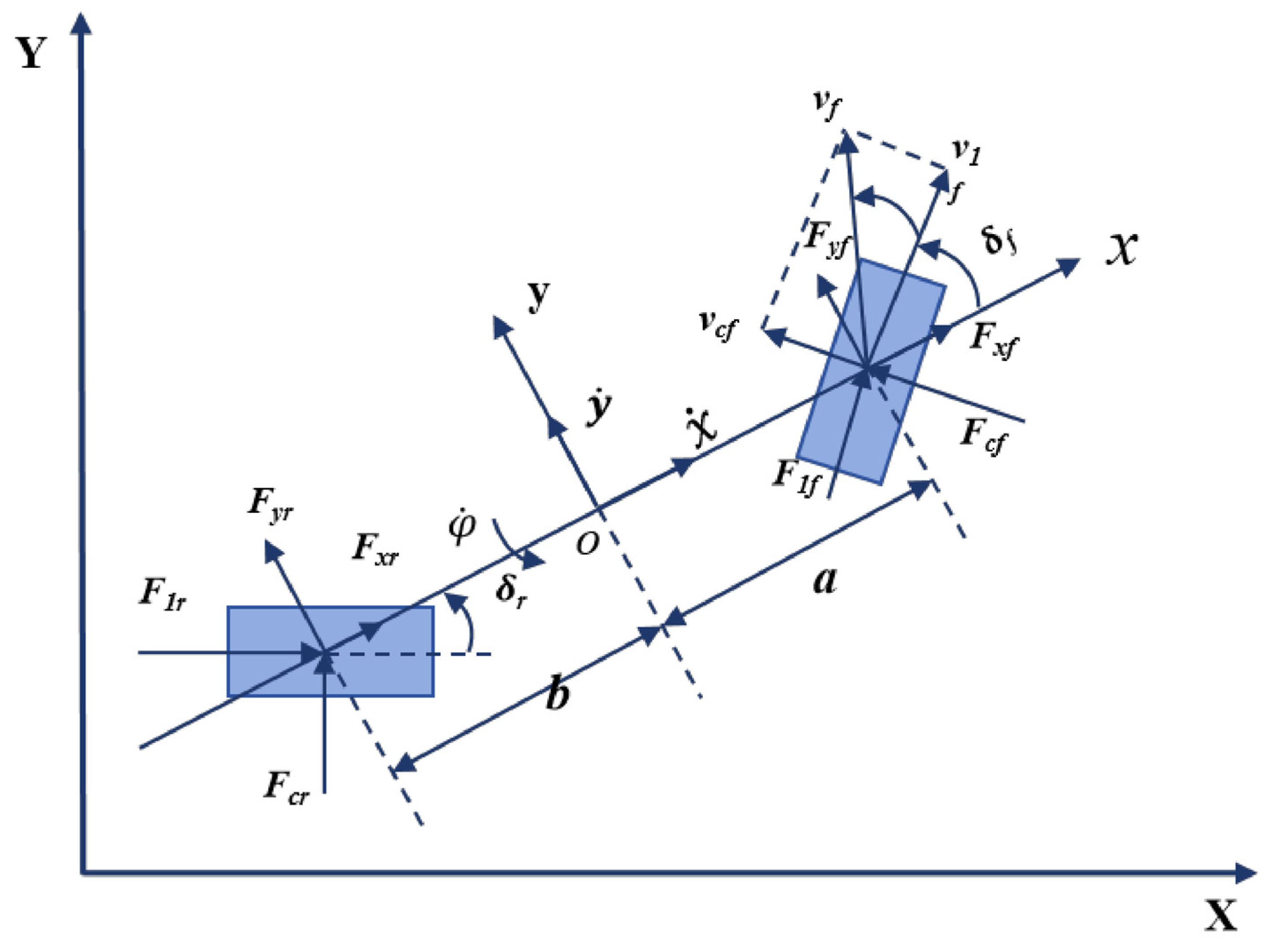
2. Vehicle Dynamics Model

The development of both kinematic and dynamic models for vehicles forms the foundational basis for analyzing intelligent vehicle control systems and designing controllers. In alignment with the precision and computational efficiency demanded by the path tracking control system, the magic formula tire model and a single-track nonlinear dynamics model for the vehicle are constructed.

2.1. Magic Formula Tire Model

The tire is the only contact point between the vehicle and the road surface, which is the medium of the vehicle transmission drive and braking forces, which directly affects the movement and performance of the vehicle. The “magic formula” (Magic Formula) tire model is widely used in the modeling and simulation of vehicle dynamics and control systems, and can accurately describe the force and torque of tires under different conditions so as to more accurately simulate the behavior of the vehicle under different conditions [17]. The magic formula tire model is usually expressed using this formula:

$$Y\left(x\right)=Dsin\left\{Carctan\left[\left(1-E\right)Bx+E{tan}^{-1}\left(Bx\right)\right]\right\}$$

(1)

where $Y\left(x\right)$ is the output variable; x is the input variable; B is a parameter of the magic formula, affecting the nonlinear characteristics of the slip angle; C is a parameter controlling the response speed of the slip angle to the force; D is a parameter representing the vertical stiffness of the tire; and E is a parameter used to introduce additional nonlinear characteristics of the tire.

When the tire side angle and the longitudinal slip rate meet the condition of its small value, the tire force can be approximated by linear relationship, and in the lateral acceleration, the daily tire has a high fitting accuracy under the condition of the tire side angle. The calculation of the longitudinal force and the lateral force can be simplified to

$$\begin{gathered} F_l=C_{l}s \\ {F}_c=C_c\alpha \end{gathered}$$

(2)

where $C_l$ is longitudinal stiffness and $C_c$ is lateral stiffness.

2.2. Vehicle Single-Track Dynamics Model

Assuming idealized hypotheses for vehicle dynamics models helps simplify complex mathematical models, improve solvability, and make the models more applicable to practical applications and fundamental theoretical research [18]. Idealized assumptions were made in establishing the dynamics model for a path tracking control strategy:

(1) The road surface is assumed to be flat, and vertical motion is not considered.

(2) The vehicle and suspension system are assumed to be rigid, ignoring the issue of ride comfort and neglecting suspension motion.

(3) The influence of air resistance is not considered.

(4) The tires are assumed to be linear, focusing only on the pure lateral characteristics of the tires and not investigating lateral load transfer.

(5) The study object is a vehicle with a small-angle steering of the front wheels.

(6) The effect of wheelbase on turning radius is ignored, and a single-track model is used to represent the vehicle’s motion.

(7) The transfer of the front and rear axle loads is disregarded.

Based on the above assumptions, a planar vehicle single-track model covering lateral, longitudinal, and yaw motion is constructed, as shown in Figure 1.

According to Newton’s second law of motion, the force equilibrium equations along the coordinate axes for the vehicle model can be established.

The force equilibrium equation along the x-axis,

$$m\ddot{x}=m\dot{y}\dot{\phi }+2F_{xf}+2F_{\mathrm{xr}}$$

(3)

where m is the curb weight of the vehicle; $\dot{\phi }$ is the yaw angular velocity; and $F_{xf} \mathrm{and} F_{xr}$ are force x in the direction of the front and rear tires, respectively.

Based on the simplification above, the nonlinear dynamic model of the tire–vehicle can be expressed as follows:

$${\dot{\xi }}_{dyn}=f_{dyn}\left({\xi }_{dyn},u_{dyn}\right)$$

(4)

The state vector ${\xi }_{dyn}$ is defined as ${\xi }_{dyn}=[\dot{y},\dot{x},\phi ,\dot{\phi },Y,X{]}^T$, where $\dot{y}$ and $\dot{x}$ represent the velocities of the vehicle in the y-direction and x-direction, respectively. $\phi$ is the yaw angle; $F_{lf}$ and $F_{lr}$ are the longitudinal forces on the front and rear tires; and $C_{lf}$ and $C_{lr}$ are the longitudinal stiffness of the front and rear tires, respectively.

3. Controller Design

3.1. The Construction of Horizontal Tracking Control Strategy

Lateral tracking control is achieved by controlling the state variable of the steering angle of the wheels to steer the vehicle in the desired direction [19]. Using the established vehicle single-track nonlinear dynamic model as a predictive model, to reduce computational complexity and meet real-time accuracy requirements, the vehicle single-track dynamic model is linearized and discretized, constraints are set, and the objective function is defined to develop the lateral tracking control strategy.

3.1.1. Building MPC Lateral Tracking Control Strategy

The key of the MPC (model predictive control) algorithm lies in solving the optimization problem of the objective function with constraints for each time step [20]. In order to improve computational efficiency and ensure control stability, the predictive model is linearized and discretized.

(1) Linearization and discretization of the predictive model:

$$\begin{gathered} {Q^{*}(\xi ,u)=min}_{U_{t,}{\xi }_{t+1\dots }{\xi }_{i+N,t}}{\displaystyle \sum _{k=t}^{t+N}}l\left(\xi \right),u(k))+P(\xi (t+N)) \\ \begin{array}{c}\begin{array}{cc}s.t {\xi }_{k+1,t}=f\left({\xi }_{k,t},u_{k,t}\right)& k=t,\dots ,N-1\end{array}\\ \begin{array}{cc}{\xi }_{k,t}\in \chi & k=t,\dots ,N-1\end{array}\\ \begin{array}{cc}{u}_{k,t}\in \Gamma & k=t,\dots ,t+N-1\end{array}\end{array} \end{gathered}$$

(5)

where $\xi$ is the state variable; $u$ is the control variable; $\chi$ is the state variable constraint; and $\Gamma$ is the control variable constraint.

Through Equation (5), the optimal sequence $Q^{*}$ of control variables can be obtained. The foremost value in this sequence is transmitted to the system platform to achieve the anticipated steering control. At the next moment, the new state of the system observed at the current time is used to obtain an optimal control variable for this step length using the same method, thus iteratively realizing the online optimization of the control variable. However, the solution process encompasses numerous optimal variables and various constraint conditions, resulting in a significant computational workload. Therefore, to reduce the computational effort and enhance the system’s real-time performance, it is necessary to apply an approximate linearization method to the established vehicle–tire prediction model.

Applying a fixed control input $u_{\mathrm{random}}$ to the model within the prediction horizon $N_c$, we obtain the system state variable ${\xi }_{\mathrm{random} }$.

$${\dot{\xi }}_{\mathrm{random} }=f\left({\xi }_{\mathrm{random} ,}{u}_{\mathrm{random} }\right)$$

(6)

At this point, by performing a first-order Taylor expansion of the established nonlinear dynamic state equation and neglecting higher-order terms, we can obtain a linear time-varying error model for the dynamics.

$${\dot{\tilde{\zeta }}}_{dyn}=A_{dyn}(t){\tilde{\xi }}_{dyn}(t)+B_{dyn}(t){\tilde{u}}_{dyn}(t)$$

(7)

Equation (7) is discretized using the method of first-order finite differences:

$${\tilde{\xi }}_{dyn}(k+1)=A_{dyn}(k){\tilde{\xi }}_{dyn}(k)+B_{dyn}(k){\tilde{u}}_{dyn}(k)$$

(8)

$$A_{dyn}(k)=I+T{A}_{dyn}(t)$$

(9)

where $I$ is the identity matrix and $T$ is the sampling time length.

To calculate the future output of the system, we define $\xi (k)=\left[\begin{array}{c}\tilde{\xi }(k)\\ \tilde{u}(k-1)\end{array}\right]$ to obtain the new state space expression:

$$\xi (k+1)={\tilde{A}}_k\xi (k)+{\tilde{B}}_k\mathsf{\Delta }u(k)$$

(10)

$$\eta (k)={\tilde{C}}_k(k)$$

(11)

where ${\tilde{A}}_k=\left[\begin{array}{cc}{A}_k& B_k\\ 0& I\end{array}\right]$ is the state transition matrix of the discrete system; ${\tilde{B}}_k=\left[\begin{array}{c}{B}_k\\ I\end{array}\right]$ is the gain matrix of the control increment for the discrete system; ${\tilde{C}}_k=\left[\begin{array}{cc}{C}_k& 0\end{array}\right]$ is the output gain matrix; $\xi \left(k\right)$ is the state variables of the discrete system; and $\eta \left(k\right)$ is the output variable of the discrete system.

According to Equation (11), the output of the system in the predictive time $N_p$ domain can be obtained as:

$$\begin{array}{c}\eta (k+1)={\tilde{C}}_k\xi (k+1)\\ ={\tilde{C}}_k{\tilde{A}}_k\xi (k)+{\tilde{C}}_k{\tilde{B}}_k\mathsf{\Delta }u(k)\\ \begin{array}{c}\&\eta (k+2)={\tilde{C}}_k{\tilde{A}}_k\xi (k+1)+{\tilde{C}}_k{\tilde{B}}_k\mathsf{\Delta }u(k+1)\\ ={\tilde{C}}_k{\tilde{A}}_k^2\xi (k)+{\tilde{C}}_k{\tilde{A}}_k{\tilde{B}}_k\mathsf{\Delta }u(k)+{\tilde{C}}_k{\tilde{B}}_k\mathsf{\Delta }u(k+1)\\ \begin{array}{c}⋮\\ \begin{array}{c}\&\eta \left(k+N_p\right)={\tilde{C}}_k{\tilde{A}}_k\xi \left(k+N_p-1\right)+{\tilde{C}}_k{\tilde{B}}_k\mathsf{\Delta }u\left(k+N_p-1\right)\\ ={\tilde{C}}_k{\tilde{A}}_k^{N_P}\xi (k)+{\tilde{C}}_k{{\tilde{A}}_k}^{N_p-1}{\tilde{B}}_k\mathsf{\Delta }u(k)+\cdots +{\tilde{C}}_k{\tilde{B}}_k\mathsf{\Delta }u\left(k+N_P-1\right)\end{array}\end{array}\end{array}\end{array}$$

(12)

Equation (12) is represented in matrix form.

$$Y=\psi \xi (k)+\Theta \mathsf{\Delta }U$$

(13)

$$\mathsf{\Delta }U={\left[\begin{array}{cccc}\mathsf{\Delta }u(k)& \mathsf{\Delta }u(k+1)& \cdots & \mathsf{\Delta }u\left(k+N_c\right)\end{array}\right]}^T$$

(14)

Through Formula (13), it can be seen that within a certain prediction horizon $N_p$, if the current state variables $\xi \left(k\right)$ of the system and the control increments $\mathsf{\Delta }U$ are known, the future output of the system at the future time can be obtained, realizing the predictive function among the three major factors in model predictive control.

(2) Establishment of the objective function.

When constructing a lateral tracking control strategy based on model predictive control (MPC), a dynamic model with higher complexity compared to a kinematic model is used in the prediction model. In order to improve the vehicle’s driving stability, enhance tracking accuracy to prevent model failure, and set corresponding control quantities and dynamic-related constraints, one might encounter high constraints during the process. This could lead to difficulties in calculating the optimal results within the predefined time. To address this issue, a relaxation factor term is added to the objective function, as shown in Formula (15):

$$\begin{array}{c}J\left({\xi }_{dyn}\left(t\right),u_{dyn}\left(t-1\right),\mathsf{\Delta }{U}_{dyn}\left(t\right)\right)\\ ={\displaystyle \sum _{i=1}^{N_p}}{‖{\eta }_{dyn}\left(t+i∣t\right)-{\eta }_{dyn,ref}\left(t+i∣t\right)‖}_Q^2{\displaystyle \sum _{i=1}^{N_c-1}}{‖\mathsf{\Delta }{u}_{dyn}\left(t+i∣t\right)‖}_R^2+\rho {\epsilon }^2\end{array}$$

(15)

where $N_p$ is the prediction horizon; $N_c$ is the control horizon; $\left(t+i\left|t\right.\right)$ is the information at time t that predicts the value at time; ${\eta }_{dyn}\left(t+i\left|t\right.\right)$ is the predicted output value; ${\eta }_{dyn,ref}\left(t+i\left|t\right.\right)$ is the reference output value; $\mathsf{\Delta }{u}_{dyn}\left(t+i\left|t\right.\right)$ is the control increment at time; and $N_c-1$,$Q,R,\rho$, and ρ are weight coefficient matrices.

Defining the reference output as $Y_{\mathrm{ref} }={\left[{\eta }_{\mathrm{ref} }(k+1),\cdots ,{\eta }_{\mathrm{ref} }\left(k+N_p\right)\right]}^T$, the deviation between the reference value and the output value is given by $E=\psi \xi (k)-Y_{ref}=\psi \xi (k)$.

The expression for quadratic programming is as follows:

$$\begin{array}{c}\underset{\mathsf{\Delta }u,\epsilon }{min}\frac{1}{2}{X}^{T}HX+G^{T}X\\ \begin{array}{c}s.t. AX\le b\end{array}\\ lb\le X\le ub\end{array}$$

(16)

In the expression, $A=\left[\begin{array}{ccccc}1& 0& \cdots & \cdots & 0\\ 1& 1& 0& \cdots & 0\\ 10& 1& 1& \ddots & 0\\ ⋮& ⋮& \ddots & \ddots & 0\\ 1& 1& \cdots & 1& 1\end{array}\right]\otimes I_m$, where $\otimes$ denotes the Kronecker product and $m$ controls the number of control variables.

Thus, based on model predictive control (MPC), the lateral tracking problem has been transformed into a standard quadratic programming problem, where the objective is to solve for the system control variables at each time step.

$$\begin{array}{c}{}_{△u}{}^{min}\frac{1}{2}{X}^{T}HX+G^{T}X\\ s.t. △U_{min}\le △U\le △U_{max}\\ U_{min}\le A△U+U_t\le U_{max}\end{array}$$

(17)

Based on the above theory, the lateral path tracking control process is transformed into a system where the control increments for each time step are calculated to obtain the corresponding control variables. The vehicle system executes the calculated control variables for the current time step, and similarly, calculates the system control variables for the next time step. This process repeats continuously, ultimately achieving the control objective of tracking the predefined path.

Considering the actual constraints, the objective function can be formulated as follows:

$$\left\{\begin{array}{c}{}_{{△U}_{dy,\epsilon }}{}^{min}={\displaystyle \sum _{i=1}^{N_p}}{‖{\eta }_{dyn}\left(t+i\right|t)-{\eta }_{dyn,ref}\left(t+i\right|t)‖}_Q^2+{\displaystyle \sum _{i=1}^{N_c}}{‖△u_{dyn}\left(t+i\right|t)‖}_R^2+\rho {\epsilon }^2\\ \begin{array}{ll}s.t. & {△U}_{dyn,min}\le {△U}_{dyn,t}\le {△U}_{dyn,max}\end{array}\\ \begin{array}{c}{△U}_{dyn,min}\le {△AU}_{dyn,t}+U_{dyn,t}\le {△U}_{dyn,max}\\ y_{hc,min}\le y_{hc}\le y_{hc,max}\\ \begin{array}{c}{y}_{sc,min}-\epsilon \le y_{sc}\le y_{sc,max}+\epsilon \\ \epsilon >0\end{array}\end{array}\end{array}\right.$$

(18)

where $y_{hc}$ is hard constraints on the output amount; $y_{sc}$ is soft constraints on the output quantity; ${y_{hc},max}_{hc,min}$ is the highest value of the output hard constraint; and $y_{sc,min},y_{sc,max}$ is the limit value of the output quantity soft constraint.

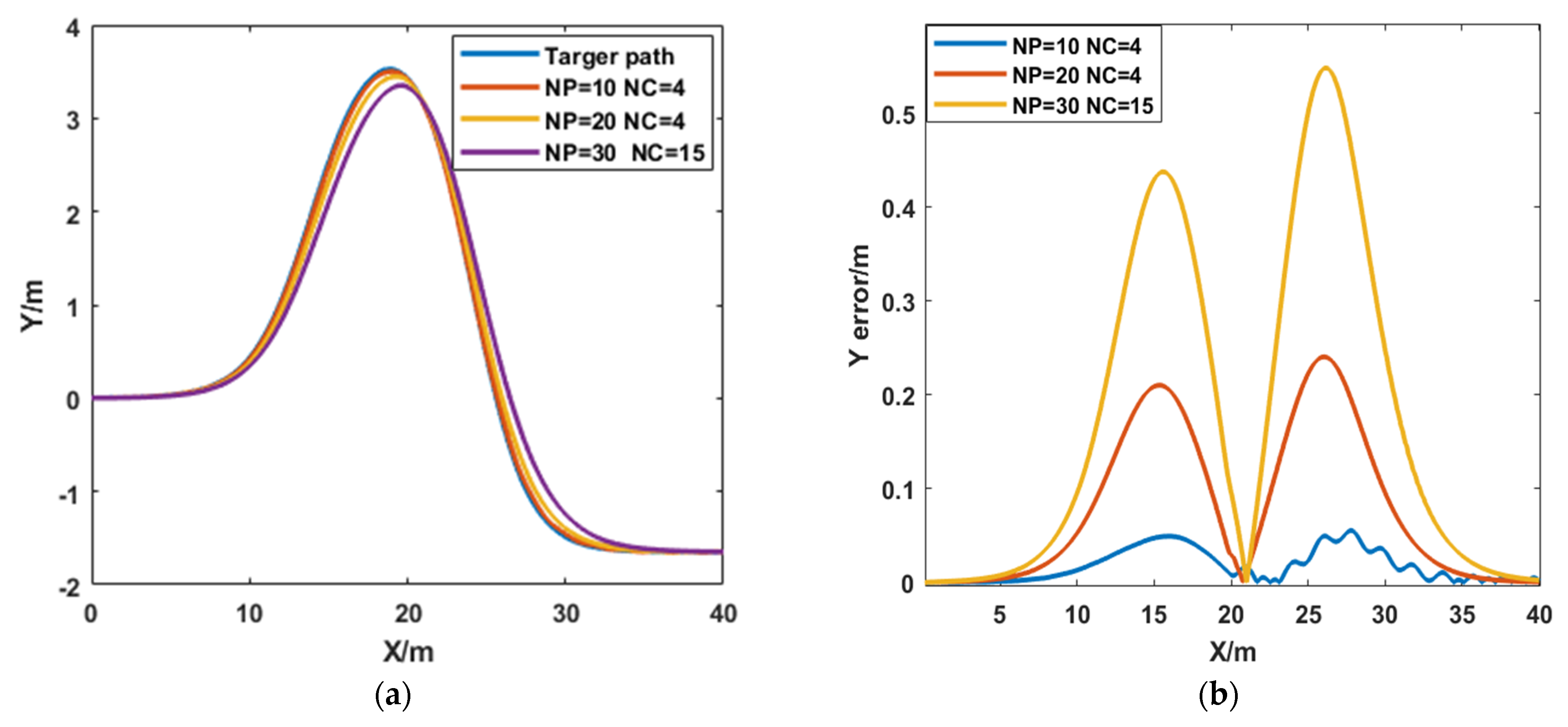
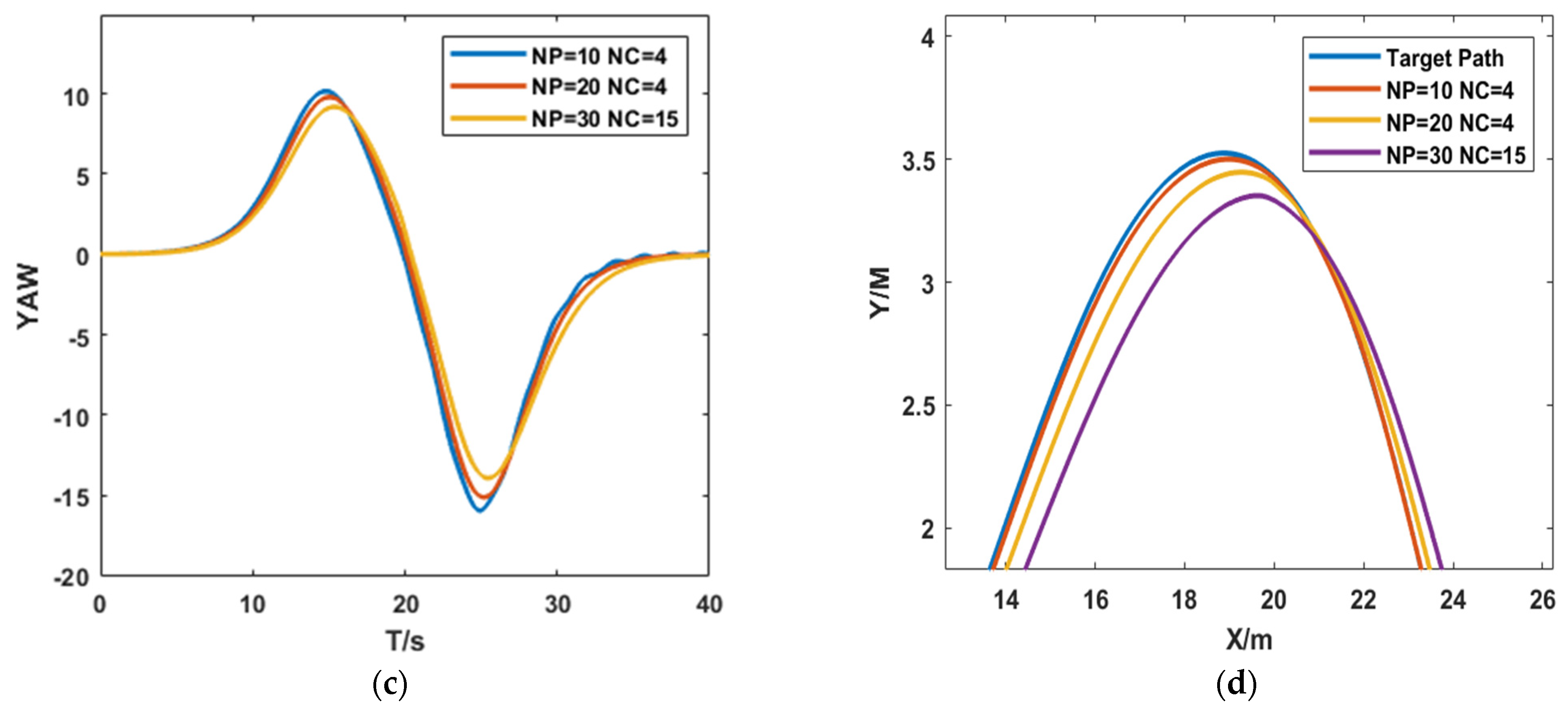
3.1.2. Analyzing the Impact of NPNC on Tracking Control Effectiveness

The article utilizes a model predictive control lateral tracking control strategy, where the selection of the parameter prediction time-domain NP and the control time-domain NC is generally based on experience, which has a strong subjectivity. To investigate the impact of NPNC on the model tracking accuracy, the article selects a daily dry asphalt double-lane working condition road, with a road surface adhesion coefficient set to 0.85 and a vehicle speed set to 10 km/h, to observe the tracking results of different NPNCs. The experimental results are shown in Figure 2 and

Table 1. Horizontal tracking error table.

NP/NC	NP = 10 NC = 4	NP = 20 NC = 4	NP = 30 NC = 15
Average tracking error (m)	0.01765	0.07917	0.1763
Maximum tracking error (m)	0.05546	0.2405	0.5485

.

From Figure 2a, it can be seen that when the vehicle is tracking the desired double-lane trajectory on a dry asphalt road at a low speed of 10 m/s, it exhibits better tracking accuracy when the prediction time domain is 10 and the control time domain is 4, as well as when the prediction time domain is 20 and the control time domain is 4. The error Figure 2b also indicates that under these parameters, the tracking error is at the centimeter level, with a maximum tracking error of about only 5 cm. From the lateral angle variation graph in Figure 2c, it can be observed that in these two cases, the lateral angle values are within the constrained range and exhibit a smooth and stable change, indicating good tracking stability. However, when the prediction time domain is 30 and the control time domain is 15, the tracking accuracy deteriorates from the previous centimeter level to the decimeter level, with a maximum tracking error of about 54 cm and poor stability, not meeting the requirements of tracking accuracy.

In addition, from the path tracking local magnification diagram in Figure 2d, it is evident that the variation in the internal time-domain parameters within the lateral tracking control strategy based on the MPC algorithm will affect the vehicle system’s tracking results of the target path. The designed model predictive lateral tracking control strategy can achieve tracking of the desired path under certain fixed conditions. However, as the internal parameters in the control strategy are fixed values once they are set, different tracking effects will occur under different driving conditions. This indicates that the designed lateral path tracking control strategy needs to improve its adaptability and robustness to changes in external environmental conditions and its own parameters.

Therefore, this paper uses a BP neural network model to select the NPNC parameters in the MPC tracking control algorithm, enabling the tracking system to adaptively select the system’s time-domain parameters based on the driving conditions to improve tracking accuracy.

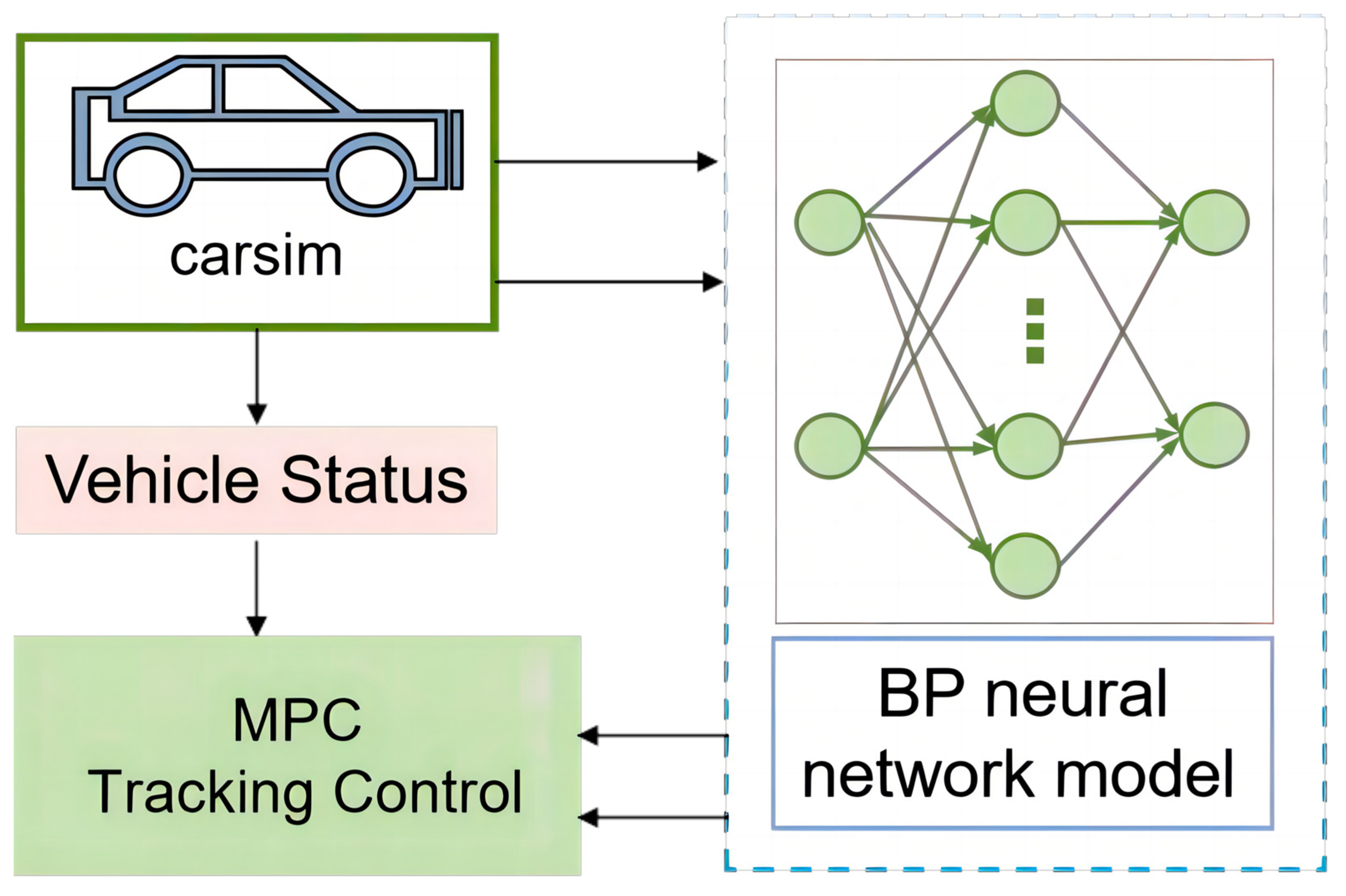
3.1.3. Build a BP Neural Network Simulation Model

In order to enhance the robustness of the system to external condition variations, a BP neural network model is used to determine the NPNC parameters in the MPC tracking control algorithm. The trained BP neural network can possess associative memory and predictive capabilities. The construction and training process is as follows:

Based on the composition of the neural network system, specify the number of neurons $n, l, m$ in each layer. Assign preset values to the connection weights between neurons, the thresholds a and b for the hidden layer and output layer. Set the learning rate $\eta$ and activation function $f\left(x\right)$. In this text, we use the Sigmoid function, $f(x)=\frac{1}{1+e^{-x}}$. When the sample error exceeds the predefined threshold, the gradient descent method is used to minimize the error function. The weight update formula is

$$w_{ij}=w_{ij}+\eta H_j\left(1-H_j\right)x_i{\displaystyle {\sum }_{k=1}^m}{w}_{jk}{e}_k$$

(19)

According to the above theory, as the input layer of the neural network consists of vehicle speed and adhesion coefficient, it has two neurons. The output layer represents the prediction horizon and control horizon, so it also has two neurons. The number of hidden layers will affect the model’s prediction accuracy and response time. After multiple experiments, the number of neurons in the hidden layer is set to 10, establishing a network layout of 2-10-2. The learning rate is set to 0.001, with 1000 iterations, and the training function is set to “trainlm”.

Using the lateral tracking control model built in CarSim/MATLAB, the magic tire model built for CarSim, type 225/60R18 tire, simulate tests at different speeds on dry asphalt roads (road adhesion coefficient set to 0.85), wet roads (road adhesion coefficient set to 0.5), and icy/snowy roads (road adhesion coefficient set to 0.3) to obtain time-domain parameter values for optimal control under corresponding conditions. When the road surface is icy/snowy, speed is generally restricted, with speeds ranging from 5 km/h to 30 km/h at 5 km/h intervals. When the road surface is wet and slippery, speed limits are imposed, with speeds ranging from 20 km/h to 80 km/h at 10 km/h intervals. When the road surface is dry asphalt, speeds ranging from 10 km/h to 120 km/h are selected at 10 km/h intervals. Due to the possibility of different output values having the same control effect, there may be multiple sets of time-domain parameter values yielding the same effect under a certain speed and adhesion condition, as shown in

Table 2. Sample data.

Adhesion Coefficient	Speed	${\mathbf{N}}_{\mathbf{p}}$	${\mathbf{N}}_{\mathbf{c}}$
0.85	20	12	2
0.85	20	12	3
0.85	20	12	5
0.85	30	14	2
⋮	⋮	⋮	⋮
⋮	⋮	⋮	⋮
0.3	25	14	5
0.3	30	14	2
0.3	30	14	10

.

Finally, using the gensim function, the trained neural network is converted into a BP neural network module based on the optimized lateral tracking strategy of the BP neural network, as shown in Figure 3.

3.2. Design of Longitudinal Velocity Tracking Strategy

Build PID Speed Tracking Strategy Control

During the operation of the vehicle system, simultaneous acceleration and deceleration control is not allowed, as it can lead to brake failure and damage to the powertrain and transmission system. In the design of the longitudinal speed controller, besides the requirement that the braking system and power system should not work together, it also stipulates that the acceleration and deceleration switching should not be too frequent to protect the vehicle’s actuator and improve ride comfort. Therefore, the acceleration and deceleration control quantity can be represented by the following formula:

$$\alpha =\left\{\begin{array}{cc}{\lambda }_{a}u& \left|e\right|\ge \left|e_0\right|\hspace{1em}u>0\\ {\alpha }_{sat}& \left|e\right|\ge \left|e_0\right|\hspace{1em}u>0\hspace{1em}{\lambda }_{a}u>{\alpha }_{sat}\end{array}\right.$$

(20)

$$p=\left\{\begin{array}{cc}{\lambda }_{b}u& \left|e\right|\ge \left|e_0\right|\hspace{1em}u<0\\ p_{sat}& \left|e\right|\ge \left|e_0\right|\hspace{1em}u<0\hspace{1em}{\lambda }_{b}u>p_{sat}\end{array}\right.$$

(21)

where $u$ is the control quantity output by the controller; $\alpha$ is the throttle opening;$p$ is the main cylinder pressure; ${\lambda }_a$ and ${\lambda }_b$ are the proportional coefficients for the acceleration control and braking control; and ${\alpha }_{sat}$ and $p_{sat}$ are the maximum threshold values set for the corresponding quantities.

4. Simulation Experiments and Analysis

To validate the proposed method, a joint simulation using Simulink/vehiclesim is utilized. Different road environments are set up in vehiclesim, and the real-time transmission of the vehicle’s front-wheel steering angle information from Simulink to vehiclesim is established to meet the experimental verification requirements. The experiments mainly consist of ① lateral tracking optimization validation; ② control strategy tracking performance validation; and ③ local obstacle avoidance function validation. For the lateral tracking optimization validation, the road conditions are set to dry asphalt with double-lane-shift conditions, with a road grip coefficient of 0.85. For the control strategy tracking performance validation, dry asphalt road conditions with straight lane and road grip coefficients of 0.85 are used, as well as dry asphalt road conditions with double-lane shift and a wet rainy road surface with a road grip coefficient set to 0.5, and a muddy icy road surface with a road grip coefficient set to 0.3. For the local obstacle avoidance function validation, a dry asphalt road surface with double-lane shift control is selected, with a road grip coefficient set to 0.85.

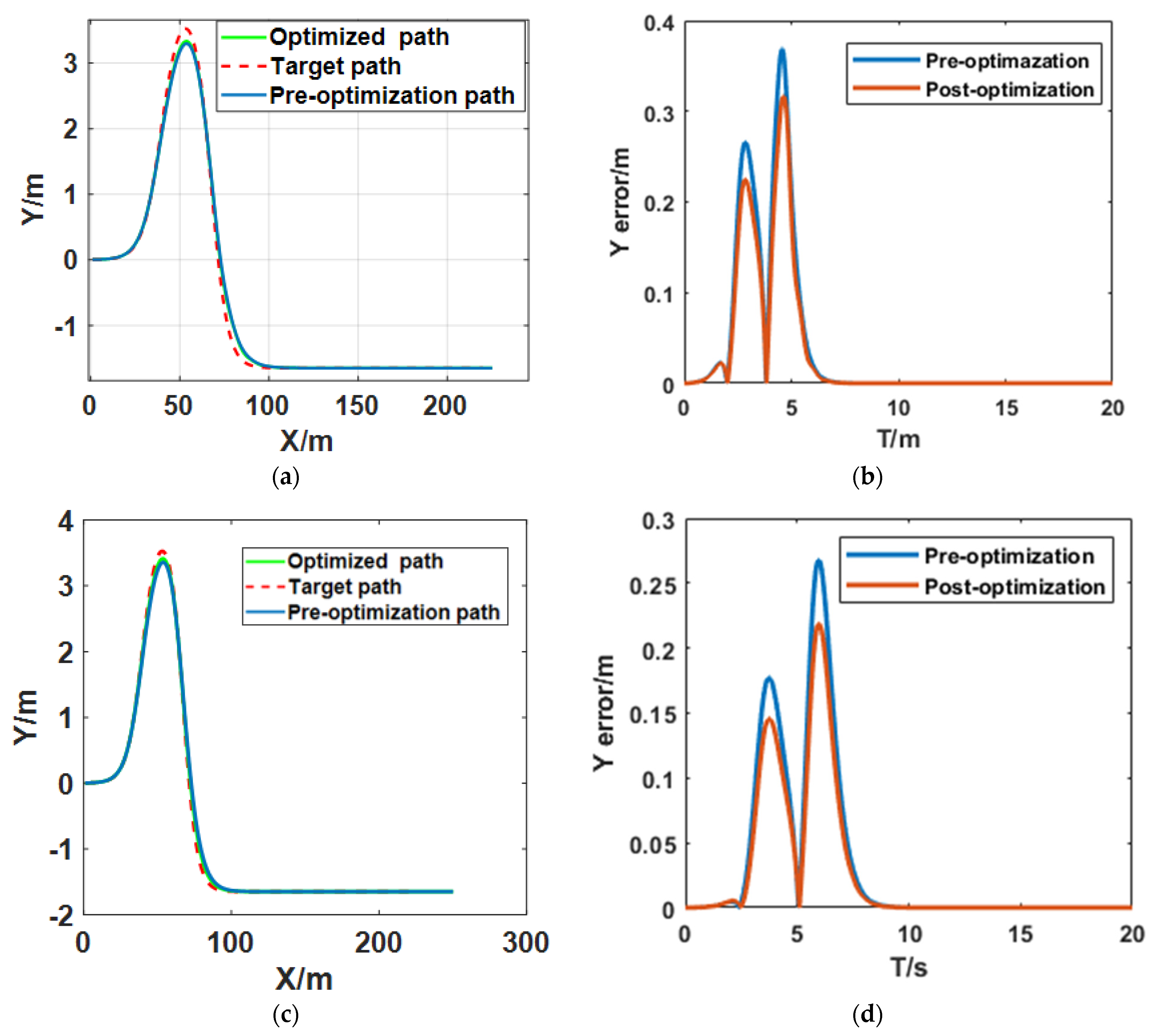
4.1. Lateral Tracking Control Optimization Validation

To validate the performance of the BP neural network optimized model for predicting lateral tracking control strategies, simulation experiments are conducted under dual-lane-shift road scenarios with different road adhesion conditions and speed settings. The dual-lane-shift test is a test method for handling performance developed by German vehicle manufacturers, which can demonstrate the vehicle’s control performance and ride comfort performance well. Therefore, this section uses dual-lane-shift conditions to verify the tracking performance after optimizing the BP neural network model.

$$\begin{array}{c}{Y}_{ref}(X)=\frac{C}{2}[1+\mathit{tanh}(E)]-\frac{D}{2}[1+\mathit{tanh}(F)]\\ {\phi }_{ref}\left(X\right)=\mathit{arctan}\left[D{\left(\frac{1}{\mathit{cosh}(E)}\right)}^2\left(\frac{1.2}{A}\right)-D{\left(\frac{1}{\mathit{cosh}(F)}\right)}^2\left(\frac{1.2}{B}\right)\right]\end{array}$$

(22)

where A = 25, B = 21.95, C = 4.05, D = 5.7, E = $\frac{2.4}{25}(X-27.19)-1.2$, and F = $\frac{2.4}{21.95}(X-56.46)-1.2$.

The aforementioned dual-lane-shift path tracking simulation is performed under different experimental conditions, simulating a dry asphalt road with a road adhesion coefficient set to 0.85, and vehicle speeds of 60 km/h and 45 km/h. The total length of the simulation road is 250 m; when the speed is 60 km/h, the simulation time is set to 15 s and when the speed is 45 km/h, the time is set to 20 s. The error before and after lateral tracking optimization at different speeds is shown in

Table 3. Comparison of Tracking Accuracy Errors before and after BP Neural Network Optimization.

Speed	60 km/h	45 km/h
Road grip coefficient	0.85	0.85
Tracking error before optimization	0.2896	0.03178
Tracking error after optimization	0.2605	0.02533
Computational time ratio before optimization ((real time)/(simulation time))	0.710067	0.5902
Computational time ratio after optimization ((real time)/(simulation time))	0.428267	0.426

and the simulation experimental results are depicted in Figure 4.

From Figure 4, it can be observed that there is a good tracking effect both before and after optimization. From Figure 4a,c it can be seen that when the vehicle speed is 60 km/h and 45 km/h, the tracking path before and after optimization basically overlaps with the desired path. There is a deviation in tracking near the right turn peaks at longitudinal distances of around 50 m and 90 m, mainly due to the increase in tracking deviation caused by the faster speed and the early turning operation on sharp curves with short path lengths. However, from Table 3, it can be seen that when the driving conditions are completely the same, the tracking errors at 60 km/h and 45 km/h are both smaller after optimization compared to before optimization. For example, at 60 km/h, the maximum lateral tracking error decreased from 0.2896 before optimization to 0.2605 after optimization; and at 45 km/h, the lateral tracking maximum error decreased from 0.03178 to 0.02533. According to the Computational time ratio, the response speed of the optimized model is faster. When the speed is 60 km/h, the simulation time is set to 15 s, and the Computational time ratio of the model decreases from 0.710067 before optimization to 0.428267; When the speed is 45 km/h, the Computational time ratio of the model decreases from 0.5902 before optimization to 0.426. The lateral tracking error graphs in Figure 4b,d show that throughout the vehicle’s operation, the tracking accuracy of the optimized model is better than that of the unoptimized model. In conclusion, the optimized lateral tracking control strategy, implemented during dual-lane-shift paths at different speeds in good road conditions, demonstrates tracking accuracy and driving stability that meet the specified constraints and safety regulations.

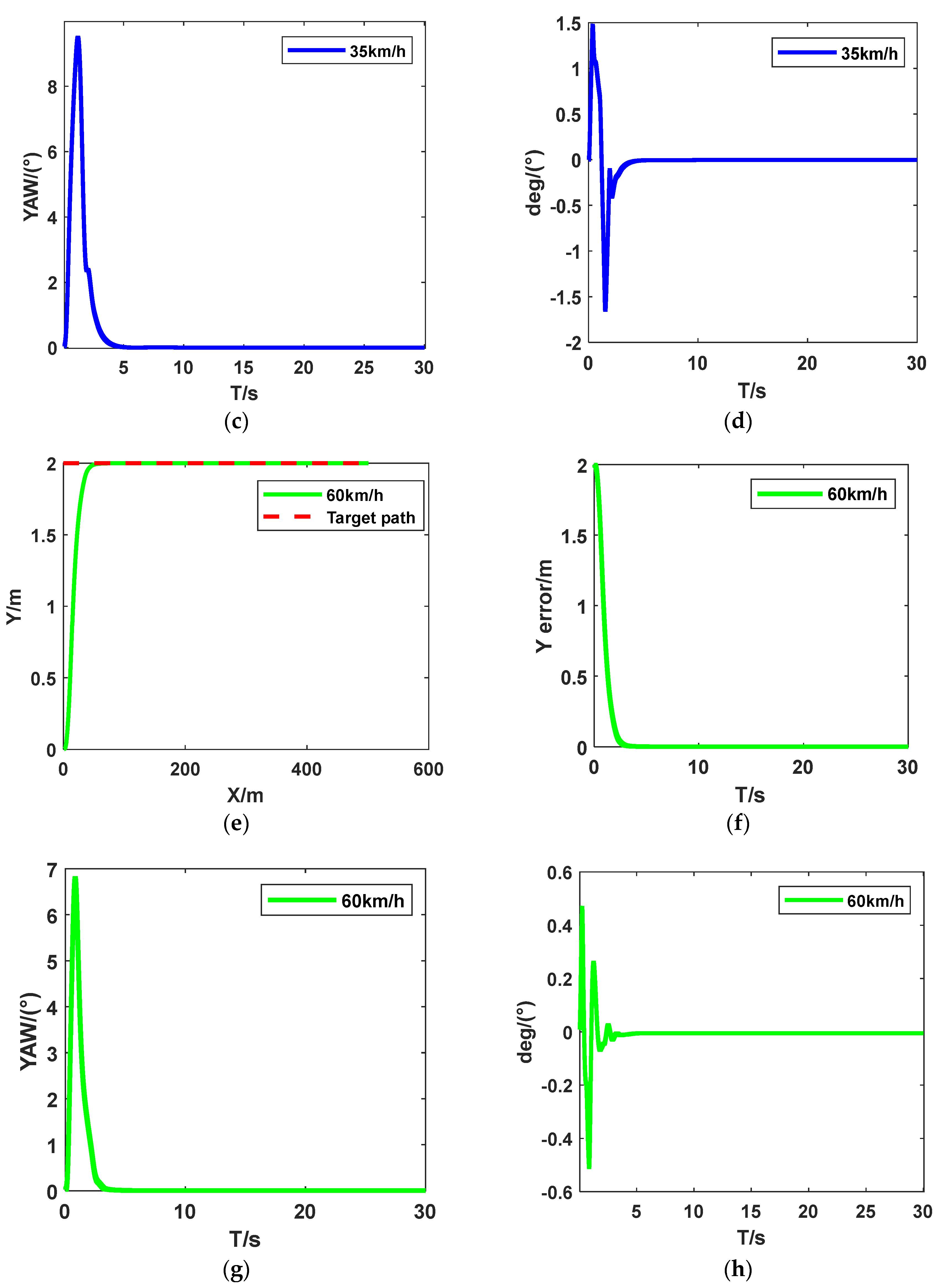
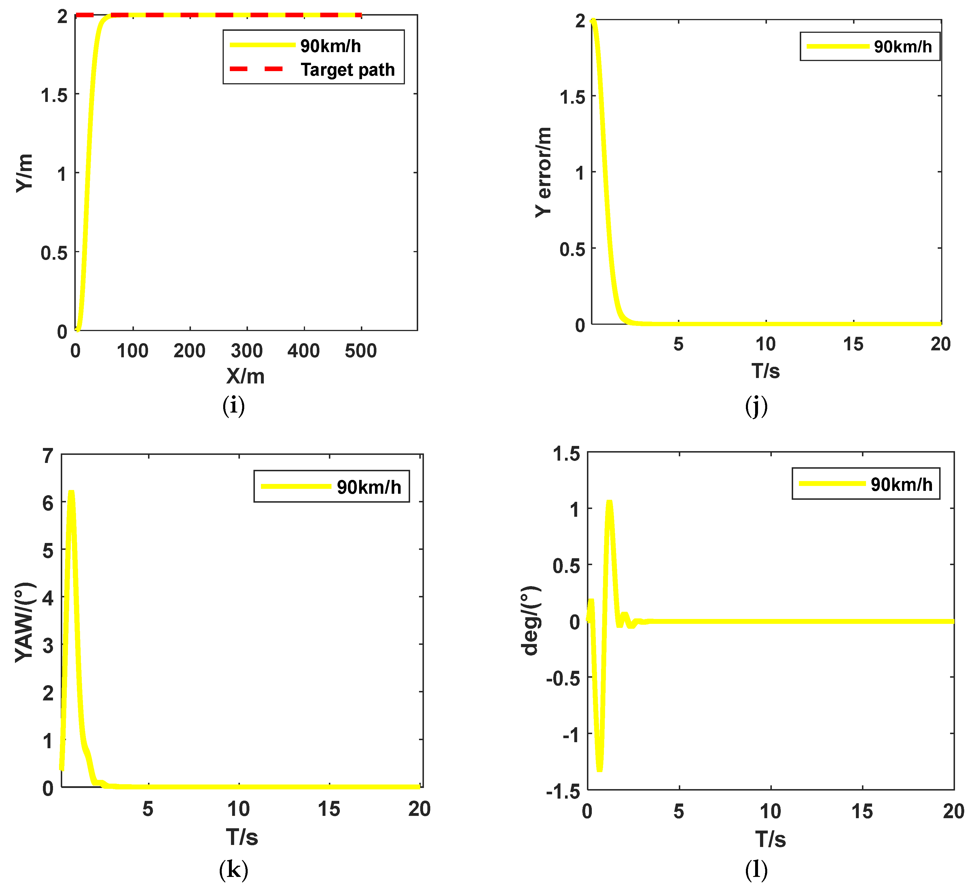
4.2. Simulation Analysis for Longitudinal and Horizontal Tracking Control Strategies

To further verify the performance of the tracking control strategy, simulation verification tests were conducted under different road conditions and various speeds, including high, medium, and low speeds. The operating conditions were categorized as straight-line conditions and dual-lane-shift conditions, with road surface conditions ranging from dry asphalt to wet rainy roads, and icy and muddy surfaces.

4.2.1. Straight-Line Conditions

Straight-line conditions are commonly used test conditions for evaluating a vehicle’s acceleration performance. The simulation experiment conditions include constant speeds of 35 km/h, 60 km/h, and 90 km/h, a dry asphalt road surface with an adhesion coefficient of 0.85, and the simulation road condition is a straight road with a 2 m lateral deviation from the vehicle’s original position, as expressed in Equation (23).

$$\left\{\begin{array}{c}{Y}_{ref}=2\\ {\phi }_{ref}=0\end{array}\right.$$

(23)

The tracking results of the straight road conditions are shown in Figure 5. It can be seen from Figure 5a,e,i that the vehicle can track the path at speeds of 35 km/h, 60 km/h, and 90 km/h. From Figure 5b,f,j, it can be observed that with a deviation distance of two meters, the vehicle can track the desired path within 2.5 s under the designed tracking control strategy, and once the vehicle reaches the longitudinal coordinate of the tracking path, the tracking error remains stable at 0. As shown in Figure 5c,g,k, as the deviation between the actual path and the desired path decreases, the lateral angle gradually decreases and stabilizes at 0 within the constraints for medium to high speeds, with the maximum value of lateral angle change being approximately 9°. The variation of the lateral deviation angle of the center of mass in Figure 5d,h,l indicates that the curve of the lateral deviation angle of the center of mass gradually stabilizes as the distance between the vehicle and the target curve decreases without any overshoot phenomenon. Therefore, it indicates that the improved tracking control strategy has higher tracking accuracy and stability for straight path tracking, meeting the requirements for driving safety.

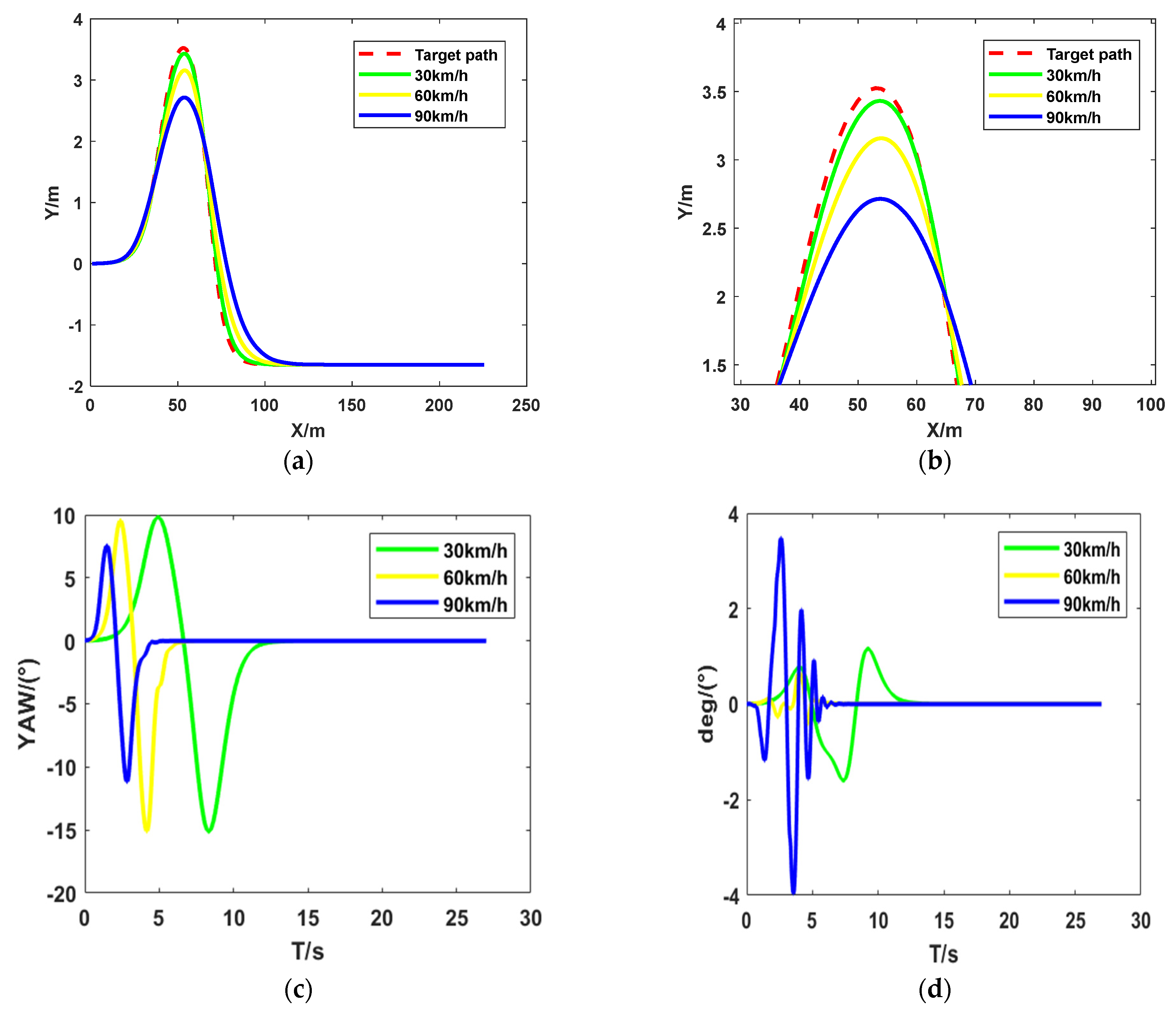
4.2.2. Biased Lane Condition

The biased lane conditions cover the experimental requirements of typical urban and highway conditions. To enhance the realism of the experiments, the road conditions are categorized based on common road surface conditions into low adhesion coefficient icy and snowy muddy roads, medium adhesion coefficient rain-slick road surfaces, and high adhesion coefficient dry asphalt roads. The specific experimental road conditions are set as follows: The desired path on dry asphalt roads is tracked at speeds of 30 km/h, 60 km/h, and 90 km/h (road adhesion coefficient set at 0.9). On rainy days, the road surface is typically wet and slippery, prone to drifting and skidding; hence, the general speed limit is below 80–90 km/h, so under wet road conditions, the desired path is tracked at speeds of 30 km/h, 60 km/h, and 80 km/h (road adhesion coefficient set at 0.5). As per regulations, the maximum speed should not exceed 30 km/h when driving on icy, snowy, or muddy roads (road adhesion coefficient set at 0.3); therefore, the vehicle speed on icy and snowy road conditions is set at 10 km/h, 20 km/h, and 30 km/h.

(1) Dry asphalt pavement.

Under the conditions of dry asphalt roads, tracking of the target path is vehicleried out at speeds of 30 km/h, 60 km/h, and 90 km/h, and the results are shown in Figure 6. It can be seen from Figure 6a,b that the tracking effect is better. At low speeds, the tracking path basically coincides with the desired path. As the vehicle speed increases, tracking deviation increases near the peak of the right turn at around 55 m longitudinally. This is mainly due to the fast speed of the vehicle and the early turning operation caused by the large curvature of the tracking curve and the short path length. When the vehicle speed is 30 km/h, the maximum tracking error is 0.2151 m with an average error of 0.0289 m; when the vehicle speed is 60 km/h, the maximum tracking error is 0.3407 m with an average error of 0.05263 m; when the vehicle speed is 90 km/h, the maximum tracking error is 0.9884 m with an average error of 0.1619 m. Although the tracking error increases with the increase in vehicle speed, the tracking error under straight-line conditions remains at 0, indicating that the tracking control strategy exhibits good tracking accuracy on dry asphalt road surfaces with good road conditions. Figure 6c shows the variation of the yaw angle during tracking under different vehicle speed conditions. The yaw angle variation range is within the designed constraint range, and the curve changes smoothly without abrupt changes. The curve of the lateral inclination angle of the center of mass in Figure 6d changes smoothly, with values ranging from −4° to 4°, within the set constraint range. On straight road segments, regardless of the vehicle speed, the center of mass lateral inclination angle and the yaw angle are stable without any fluctuations. In summary, the designed lateral tracking control strategy for path tracking under different speeds on dry asphalt road surfaces exhibits tracking accuracy and driving stability that meet the set constraints and the requirements of driving safety regulations.

(2) Wet rainy road surface.

The results of dual-lane tracking on a wet rainy road surface are shown in Figure 7. It can be seen from Figure 7a,b that the tracking path is basically aligned with the desired path, with deviation values close to 0 in the first 20 m of straight road and before entering the curve. The main tracking deviation occurs in sharp right-turn curves. When the vehicle speed is 25 km/h, the maximum tracking error is 0.2048 m with an average error of 0.02508 m; when the vehicle speed is 45 km/h, the maximum tracking error is 0.2422 m with an average error of 0.03189 m; when the vehicle speed is 85 km/h, the maximum tracking error is 0.2797 m with an average error of 0.04999 m. Although the maximum tracking error has increased by about 0.1 compared to dry asphalt road surfaces with better driving conditions, the average error has decreased, indicating a high level of tracking accuracy. From Figure 7c,d, it can be seen that both the yaw angle and the lateral inclination angle of the center of mass are within the specified constraint range. In conclusion, tracking at different speeds on a wet rainy road surface still demonstrates good stability and tracking accuracy.

(3) The road is covered with ice, snow, and mud.

Under the road surface conditions with an adhesion coefficient of 0.3 for icy and snowy roads, path tracking was conducted at speeds of 10 km/h, 20 km/h, and 30 km/h, as shown in Figure 8. It can be observed from Figure 8a,b that, due to the slower speeds, even with the lower adhesion coefficient there is a significant improvement in tracking accuracy as the vehicle enters the curve tracking at 55 m. Good tracking results can still be achieved. The maximum tracking error is 0.07569 m with an average error of 0.01289 m at a speed of 10 km/h; there is a 0.1482 m maximum tracking error and 0.02052 m average error at a speed of 20 km/h; and a 1.685 m maximum tracking error and 0.3103 m average error at a speed of 30 km/h. Both the lateral deviation angle and the yaw angle do not exceed the constraints, and all parameters change smoothly and steadily with the road conditions, meeting the stability requirements of vehicle driving. Overall, it indicates that driving at different speeds under icy and snowy conditions still maintains good stability and tracking accuracy.

In conclusion, by setting a single variable, verifying different road conditions under fixed-speed conditions, or verifying different speed conditions under fixed road conditions, the simulation results show that the real-time performance and effectiveness of the designed longitudinal and lateral coordinated path tracking controller meet the requirements.

5. Conclusions

Addressing the issue of excessive and fixed motion control model parameters in intelligent vehicles leading to poor real-time performance and inadequate tracking capabilities, this paper proposes a path tracking control strategy for intelligent driving vehicles based on a BP neural network. Firstly, for lateral tracking, the nonlinear modeling capability of neural networks and the advantages of model predictive control (MPC) are utilized. The BP neural network optimizes and improves the lateral tracking control strategy, allowing for the online adjustment of temporal parameters according to driving conditions and vehicle status. This enables more accurate control decisions in dynamic environments. Secondly, an incremental PID vehicle speed tracking controller is designed, achieving coordinated longitudinal and lateral control of the vehicle. Finally, the effectiveness of the designed longitudinal and lateral coordinated path tracking control algorithm is verified through CarSim/Simulink joint simulation. The results show that the designed path tracking control system can adaptively and dynamically select temporal parameters in the control strategy to obtain front-wheel steering angles based on different road surface adhesion coefficients and driving conditions. This balances the tracking performance and driving performance under the same conditions, thereby ensuring both tracking and driving performance during the vehicle path tracking process.

References

1. Yurtsever, E.; Lambert, J.; Carballo, A.; Takeda, K. A survey of autonomous driving: Common practices and emerging technologies. IEEE Access 2020, 8, 58443–58469. [Google Scholar] [CrossRef]
2. Zha, Y.; Deng, J.; Qiu, Y.; Zhang, K.; Wang, Y. A survey of intelligent driving vehicle trajectory tracking based on vehicle dynamics. SAE Int. J. Veh. Dyn. Stab. NVH 2023, 7, 221–248. [Google Scholar] [CrossRef]
3. AbdElmoniem, A.; Osama, A.; Abdelaziz, M.; Maged, S.A. A path-tracking algorithm using predictive Stanley lateral controller. Int. J. Adv. Robot. Syst. 2020, 17, 1729881420974852. [Google Scholar] [CrossRef]
4. Lal, D.S.; Vivek, A.; Selvaraj, G. Lateral control of an autonomous vehicle based on pure pursuit algorithm. In Proceedings of the 2017 International Conference on Technological Advancements in Power and Energy (Tap Energy), Kollam, India, 21–23 December 2017; pp. 1–8. [Google Scholar]
5. Yu, L.; Yan, X.; Kuang, Z.; Chen, B.; Zhao, Y. Driverless bus path tracking based on fuzzy pure pursuit control with a front axle reference. Appl. Sci. 2019, 10, 230. [Google Scholar] [CrossRef]
6. Li, T.; Ren, H.; Li, C. Intelligent electric vehicle trajectory tracking control algorithm based on weight coefficient adaptive optimal control. Trans. Inst. Meas. Control 2023, 01423312221141591. [Google Scholar] [CrossRef]
7. Wu, H.; Li, Z.; Si, Z. Trajectory tracking control for four-wheel independent drive intelligent vehicle based on model predictive control and sliding mode control. Adv. Mech. Eng. 2021, 13, 16878140211045142. [Google Scholar] [CrossRef]
8. Han, G.; Fu, W.; Wang, W.; Wu, Z. The lateral tracking control for the intelligent vehicle based on adaptive PID neural network. Sensors 2017, 17, 1244. [Google Scholar] [CrossRef] [PubMed]
9. Wang, S.; Hui, Y.; Sun, X.; Shi, D. Neural network sliding mode control of intelligent vehicle longitudinal dynamics. IEEE Access 2019, 7, 162333–162342. [Google Scholar] [CrossRef]
10. Yang, T.; Bai, Z.; Li, Z.; Feng, N.; Chen, L. Intelligent vehicle lateral control method based on feedforward+ predictive LQR algorithm. Actuators 2021, 10, 228. [Google Scholar] [CrossRef]
11. Yang, C.; Liu, J. Trajectory tracking control of intelligent driving vehicles based on MPC and Fuzzy PID. Math. Probl. Eng. 2023, 2023, 2464254. [Google Scholar] [CrossRef]
12. Bharali, J.; Buragohain, M. Design and performance analysis of Fuzzy LQR; Fuzzy PID and LQR controller for active suspension system using 3 Degree of Freedom quarter car model. In Proceedings of the 2016 IEEE 1st International Conference on Power Electronics, Intelligent Control and Energy Systems (ICPEICES), Delhi, India, 4–6 July 2016; pp. 1–6. [Google Scholar]
13. Tan, W.; Wang, M.; Ma, K. Research on Intelligent Vehicle Trajectory Tracking Control Based on Improved Adaptive MPC. Sensors 2024, 24, 2316. [Google Scholar] [CrossRef] [PubMed]
14. Zuo, Z.; Yang, X.; Li, Z.; Wang, Y.; Han, Q.; Wang, L.; Luo, X. MPC-based cooperative control strategy of path planning and trajectory tracking for intelligent vehicles. IEEE Trans. Intell. Veh. 2020, 6, 513–522. [Google Scholar] [CrossRef]
15. Kouvaritakis, B.; Cannon, M. Model Predictive Control; Springer International Publishing: Cham, Switzerland, 2016; Volume 38, pp. 13–56. [Google Scholar]
16. Sun, X.; Fu, J.; Yang, H.; Xie, M.; Liu, J. An energy management strategy for plug-in hybrid electric vehicles based on deep learning and improved model predictive control. Energy 2023, 269, 126772. [Google Scholar] [CrossRef]
17. Tang, L.; Yan, F.; Zou, B.; Wang, K.; Lv, C. An improved kinematic model predictive control for high-speed path tracking of autonomous vehicles. IEEE Access 2020, 8, 51400–51413. [Google Scholar] [CrossRef]
18. Ni, J.; Hu, J.; Xiang, C. A review for design and dynamics control of unmanned ground vehicle. Proc. Inst. Mech. Eng. Part D J. Automob. Eng. 2021, 235, 1084–1100. [Google Scholar] [CrossRef]
19. Yao, Q.; Tian, Y.; Wang, Q.; Wang, S. Control strategies on path tracking for autonomous vehicle: State of the art and future challenges. IEEE Access 2020, 8, 161211–161222. [Google Scholar] [CrossRef]
20. Fu, T.; Yao, C.; Long, M.; Gu, M.; Liu, Z. Overview of longitudinal and lateral control for intelligent vehicle path tracking. In Proceedings of the 2019 Chinese Intelligent Automation Conference, Jiangsu, China, 20–22 September 2019; pp. 672–682. [Google Scholar]
Figure 1. Vehicle monorail model.
Wevj 15 00185 g001
Figure 2. Comparison diagram of NPNC’s influence on tracking results: (a) tracing the result comparison chart; (b) tracking the lateral error comparison chart; (c) lateral tracking yaw angle; (d) local magnification of tracking results.
Wevj 15 00185 g002aWevj 15 00185 g002b
Figure 3. Horizontal tracking decision.
Wevj 15 00185 g003
Figure 4. Comparison of horizontal path tracking strategy before and after optimization: (a) the tracking results comparison at a speed of 60 km/h; (b) speed 60 km/h lateral tracking error comparison chart; (c) speed 45 km/h path tracking results comparison; (d) speed 45 km/h lateral tracking error comparison.
Wevj 15 00185 g004
Figure 5. Linear condition tracking results for vehicle speeds of 35 km/h, 60 km/h, and 90 km/h: (a) the speed is 35 km/h, linear condition tracking result; (b) the speed is 35 km/h, linear condition tracking error; (c) the speed is 35 km/h, under linear condition; (d) the speed is 35 km/h, linear condition tracking error; (e) the speed is 60 km/h, linear condition tracking result; (f) the speed is 60 km/h, linear condition tracking error; (g) the speed is 60 km/h, under linear condition; (h) the speed is 60 km/h, in straight-line condition; (i) the speed is 90 km/h, linear condition tracking result; (j) the speed is 90 km/h, linear condition tracking error; (k) the speed is 90 km/h, under linear condition; (l) the speed is 90 km/h, in straight-line condition.
Wevj 15 00185 g005aWevj 15 00185 g005bWevj 15 00185 g005c
Figure 6. Tracking results of double-lane-shift working conditions on dry asphalt roads: (a) tracking result; (b) local amplification of tracking results; (c) yaw angle variation trend chart; (d) trend diagram of lateral declination angle of center of mass.
Wevj 15 00185 g006
Figure 7. Tracking results of double-lane-shift condition on wet pavement: (a) tracking result; (b) local amplification of tracking results; (c) yaw angle variation trend chart; (d) trend diagram of lateral declination angle of center of mass.
Wevj 15 00185 g007
Figure 8. Tracking results of double-lane-shift condition of snow and ice muddy pavement: (a) tracking result; (b) local amplification of tracking results; (c) yaw angle variation trend chart; (d) trend diagram of lateral declination angle of center of mass.
Wevj 15 00185 g008