

Design and Construction of a Multipole Electric Motor Using an Axial Flux Configuration

Abstract
:1. Introduction
2. Materials and Methods
2.1. Axial Flux Motor Design

2.2. U-Type Coil (UC) Design
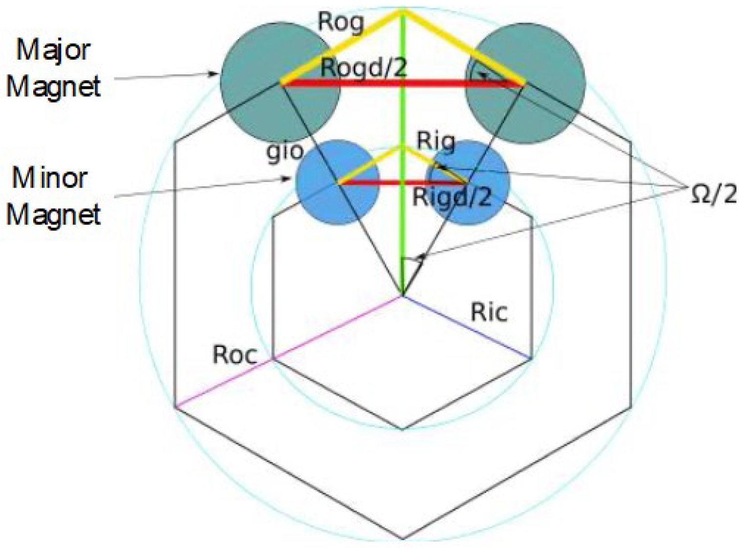
2.3. Rotor Design
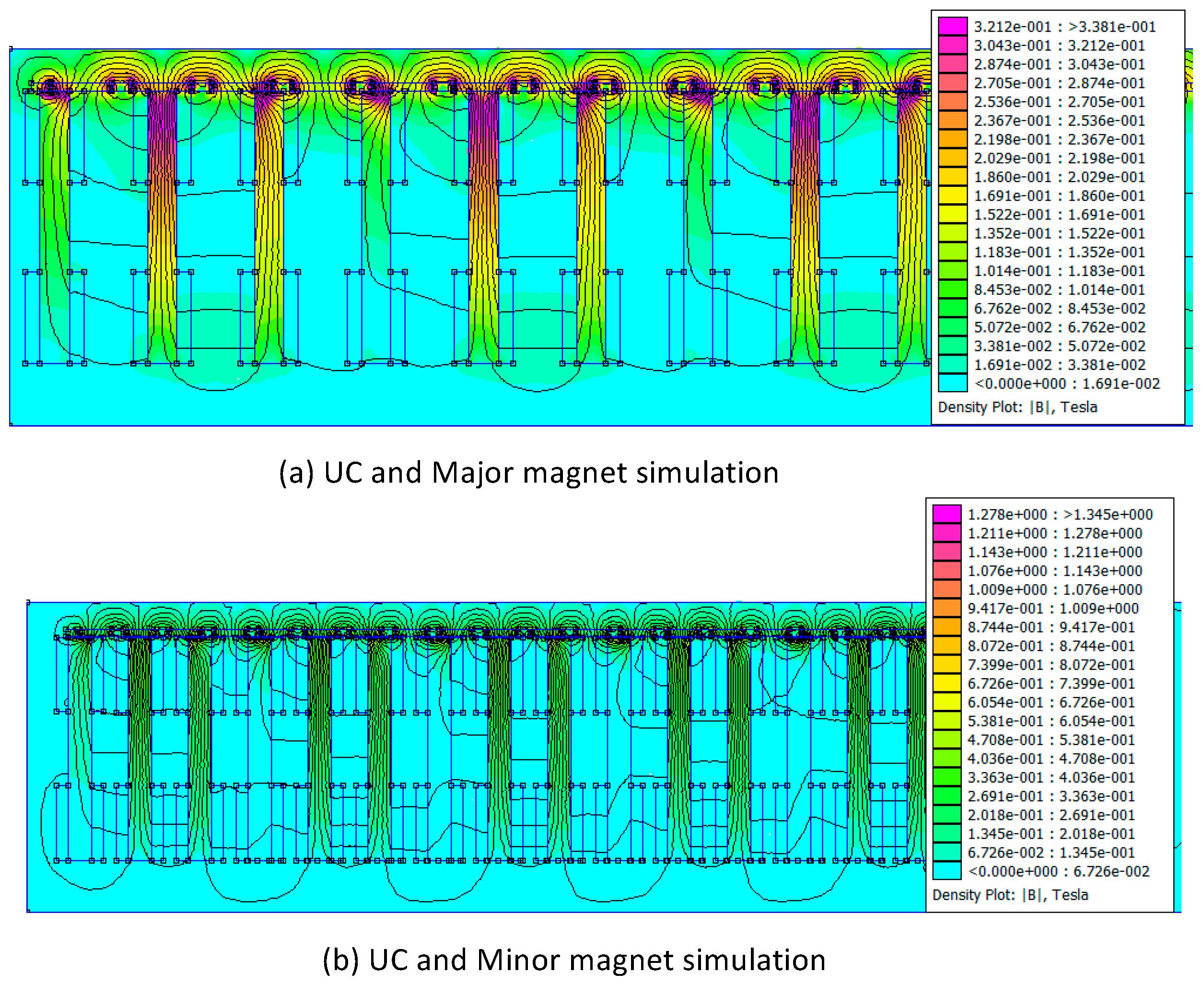
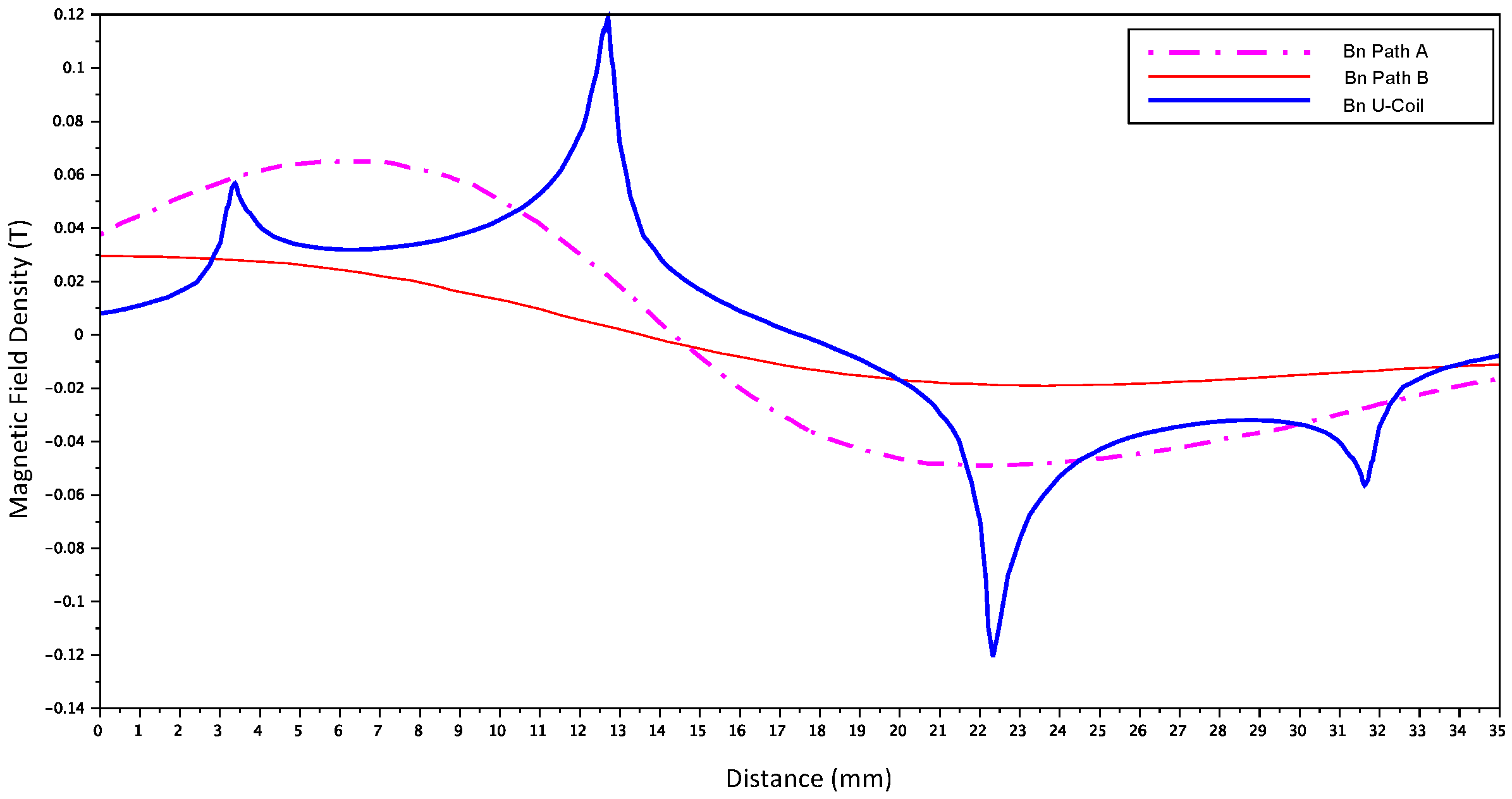
2.4. Behavior Simulation
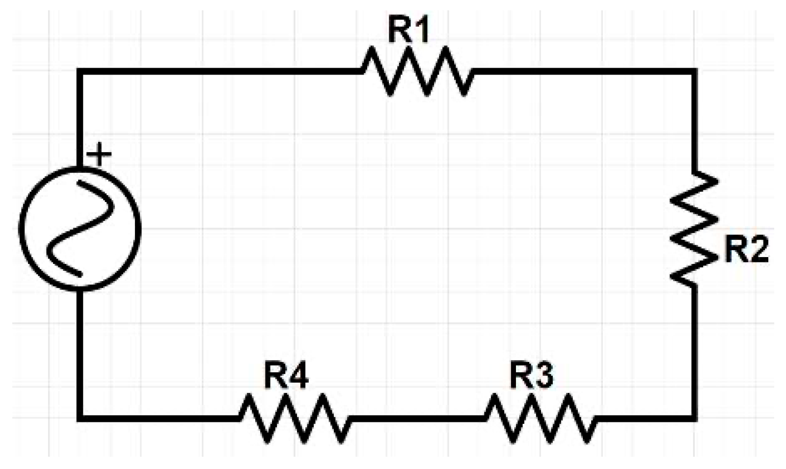
2.5. Motor Control
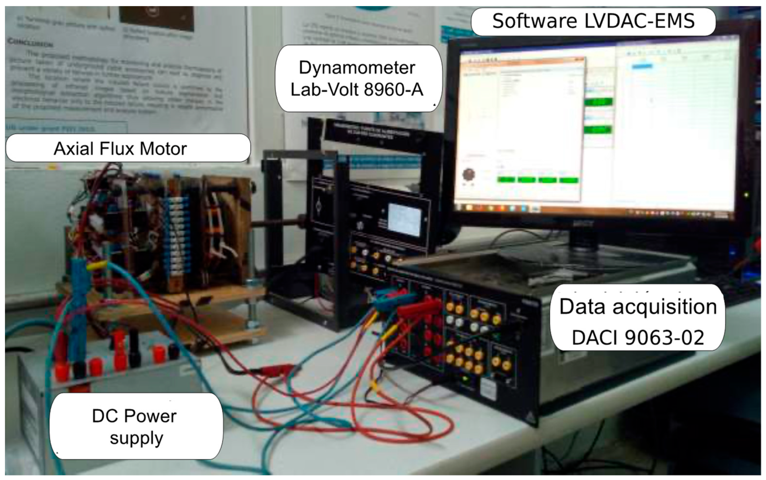
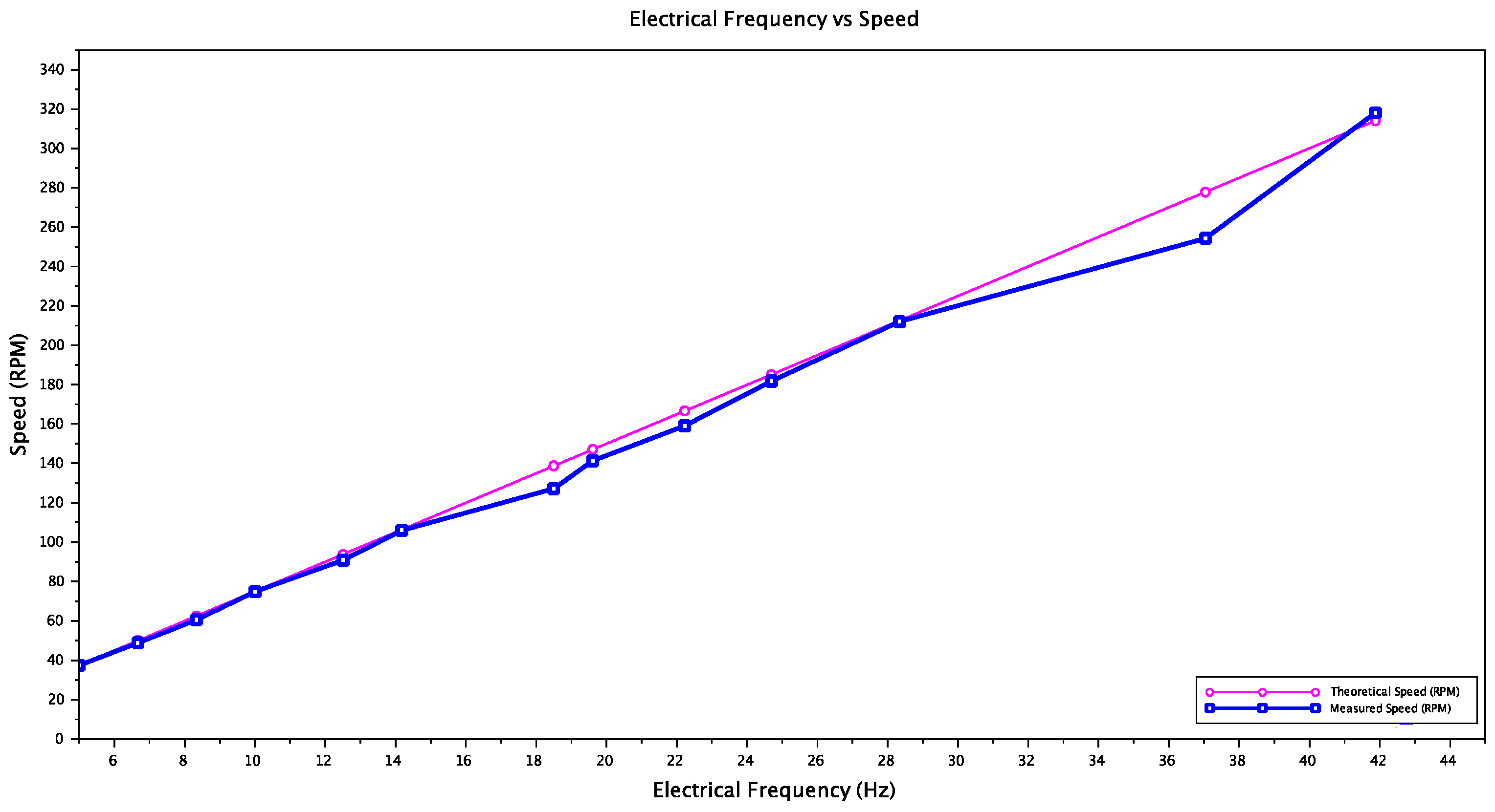
3. Results
3.1. Motor Design and Construction
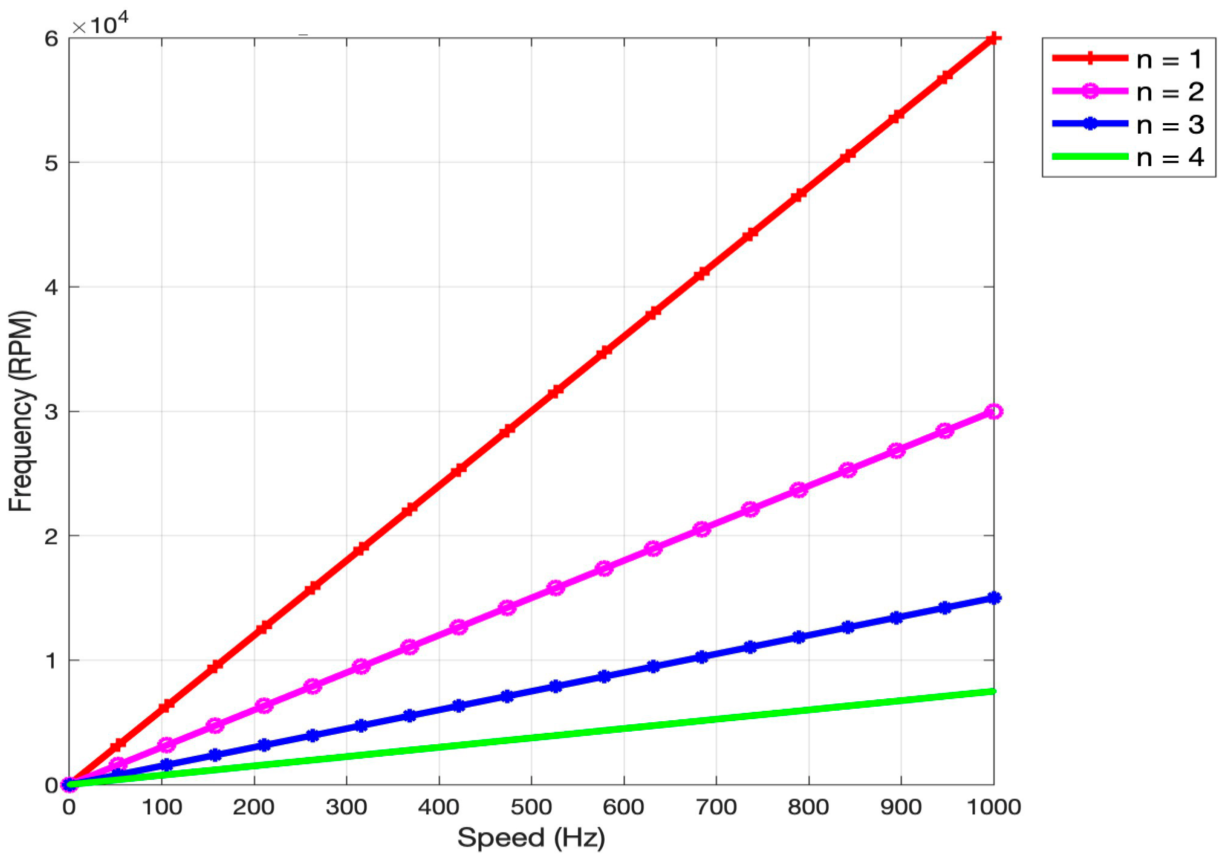
3.2. Behavior Assessment
3.3. Evaluation
4. Conclusions
Author Contributions
Funding
Data Availability Statement
Conflicts of Interest
References
- Amin, S.; Khan, S.; Bukhari, S.S.H. A Comprehensive Review on Axial Flux Machines and Its Applications. In Proceedings of the 2019 2nd International Conference on Computing, Mathematics and Engineering Technologies (iCoMET), Sukkur, Pakistan, 30–31 January 2019; pp. 1–7. [Google Scholar] [CrossRef]
- Xu, Z.; Li, T.; Zhang, F.; Zhang, Y.; Lee, D.H.; Ahn, J.W. A Review on Segmented Switched Reluctance Motors. Energies 2022, 15, 9212. [Google Scholar] [CrossRef]
- Nasiri-Gheidari, Z.; Lesani, H. A Survey on Axial Flux Induction Motors. Prz. Elektrotech. 2012, 88, 300–305. [Google Scholar]
- Gieras, F.; Wang, R.-J.; Kamper, M.J. Axial Flux Permanent Magnet Brushless Machines; Springer Science & Business Media: Berlin, Germany, 2004. [Google Scholar]
- González-Parada, A.; Lozano-García, J.M.; Ibarra-Manzano, M.A. Digital Pole Control for Speed and Torque Variation in an Axial Flux Motor with Permanent Magnets. Electronics 2022, 11, 482. [Google Scholar] [CrossRef]
- Krishnan, R.; Abouzeid, M.; Mang, X. A design procedure for axial field switched reluctance motors. In Proceedings of the Conference Record of the 1990 IEEE Industry Applications Society Annual Meeting, Seattle, WA, USA, 7–12 October 1990; Volume 1, pp. 241–246. [Google Scholar] [CrossRef]
- Materu, P.; Krishnan, R. Analytical prediction of SRM inductance profile and steady-state average torque. In Proceedings of the Conference Record of the 1990 IEEE Industry Applications Society Annual Meeting, Seattle, WA, USA, 7–12 October 1990; Volume 1, pp. 214–223. [Google Scholar] [CrossRef]
- Aydin, M.; Huang, S.; Lipo, T.A. Axial flux permanent magnet disc machines: A review. Conf. Record SPEEDAM 2004, 8, 61–71. [Google Scholar]
- Lambert, T.; Biglarbegian, M.; Mahmud, S. A Novel Approach to the Design of Axial-Flux Switched-Reluctance Motors. Machines 2015, 3, 27–54. [Google Scholar] [CrossRef]
- Shao, L.; Navaratne, R.; Popescu, M.; Liu, G. Design and construction of axial-flux permanent magnet motors for electric propulsion applications—A review. IEEE Access 2021, 9, 158998–159017. [Google Scholar] [CrossRef]
- Abdullah, H.; Ramasamy, G.; Ramar, K.; Aravind, C.V. Design consideration of dual axial flux motor for electric vehicle applications. In Proceedings of the IEEE Conference on Energy Conversion (CENCON), Johor Bahru, Malaysia, 19–20 October 2015; pp. 72–77. [Google Scholar]
- Caricchi, F.; Crescimbini, F.; Honrati, O. Modular axial-flux permanent-magnet motor for ship propulsion drives. IEEE Trans. Energy Convers. 1999, 14, 673–679. [Google Scholar] [CrossRef]
- Dianati, B.; Kahourzade, S.; Mahmoudi, A. Optimization of axial-flux induction motors for the application of electric vehicles considering driving cycles. IEEE Trans. Energy Convers. 2020, 35, 1522–1533. [Google Scholar] [CrossRef]
- Nielsen, S.S.; Jæger, R.; Rasmussen, P.O.; Kongerslev, K. Development and analysis of double U-core switched reluctance machine. In Proceedings of the IEEE International Electric Machines and Drives Conference (IEMDC), Miami, FL, USA, 21–24 May 2017. [Google Scholar] [CrossRef]
- Ostovic, V. Performance comparison of U-Core and round-stator single-phase permanent-magnet motors for pump applications. IEEE Trans. Ind. Appl. 2002, 38, 476–482. [Google Scholar] [CrossRef]
- Deng, X.; Mecrow, B.; Wu, H.; Martin, R. Design and development of low torque ripple variable-speed drive system with six-phase switched reluctance motors. IEEE Trans. Energy Convers. 2017, 33, 420–429. [Google Scholar] [CrossRef]
- Andrada Gascón, P. Design of a segmented switched reluctance drive for a light electric vehicle. Renew. Energy Power Qual. J. 2022, 20, 662–667. [Google Scholar] [CrossRef]
- Marcsa, D.; Kuczmann, M. Design and control for torque ripple reduction of a 3-phase switched reluctance motor. Comput. Math. Appl. 2017, 74, 89–95. [Google Scholar] [CrossRef]
- Kalaivani, L.; Subburaj, P.; Iruthayarajan, M.W. Speed control of switched reluctance motor with torque ripple reduction using non-dominated sorting genetic algorithm (NSGA-II). Int. J. Electr. Power Energy Syst. 2013, 53, 69–77. [Google Scholar] [CrossRef]
- Al-Amyal, F.; Hamouda, M.; Szamel, L. Performance improvement based on adaptive commutation strategy for switched reluctance motors using direct torque control. Alex. Eng. J. 2022, 61, 9219–9233. [Google Scholar] [CrossRef]
- Jæger, R.; Nielsen, S.S.; Rasmussen, P.O. Theoretical evaluation of the double U-core switched reluctance machine. In Proceedings of the 2017 IEEE International Electric Machines and Drives Conference (IEMDC), Miami, FL, USA, 21–24 May 2017. [Google Scholar] [CrossRef]


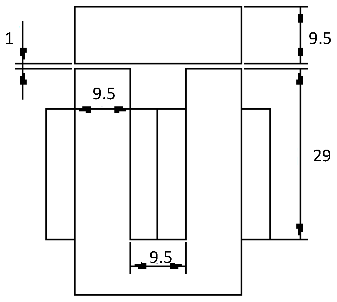
| Dimensional Design with 12/16 Poles in Stator/Rotor | ||||
|---|---|---|---|---|
| Parameters | Variable | Definition | Value | Unit |
| Input | Ul | U core length | 9.5 | mm |
| NC | Stator pole number | 12 | Parts | |
| Nm | Rotor pole number | 16 | Parts | |
| NL | Lamination number | 23 | mm | |
| EL | Lamination width | 0.5 | mm | |
| gmmd | Minimum perimeter separation between major and minor magnets | 4 | mm | |
| gmimod | Minimum separation desired between major magnet and minor magnet | 6 | mm | |
| Output | r | Radius of inscribed polygon of stator coils | 44.5 | mm |
| Ric | Radius of inscribed polygon of minor magnets | 44.8 | mm | |
| Roc | Radius of inscribed polygon of major magnets | 64.1 | mm | |
| gmin | Minimum perimeter separation between minor magnets | 4.4 | mm | |
| gmom | Minimum perimeter separation between major magnets | 5.5 | mm | |
| gmimod | Minimum separation desired between major magnet and minor magnet | 3.1 | mm | |
| Di/Ri | Minor magnet diameter | 12.7 | mm | |
| Do/Ro | Major magnet diameter | 19.0 | mm | |
| Input and Output Parameters | ||||
|---|---|---|---|---|
| Parameters | Variable | Definition | Value | Unit |
| Input | UL | Distance between U-type coils and bar (rotor) | 9.5 | mm |
| Wh | Window height | 29 | mm | |
| Wl | Window length | 9.5 | mm | |
| Uwd | Window width | 9.5 | mm | |
| EL | Lamination thickness | 0.5 | mm | |
| Nl | Lamination number | 23 | Part | |
| μm | Air relative permeability | 1 | NA | |
| μUTC | Relative core permeability | 4316 | NA | |
| μb | Relative bar (rotor) permeability | 1.04 | NA | |
| Bd | Magnetic field density | 4 | Tesla | |
| AWGCu | Copper wire gauge | 24 | AWG | |
| Output | imax | Current | 0.803 | A |
| Rc | Winding resistance | 4.77 | Ω | |
| Lc | Winding inductance | 44.89 | H | |
| Vcd | CD voltage | 3.83 | V | |
| N | Total | 376 | Part | |
| NL | Layer number | 8 | Part | |
| NCpL | Number of conductors per layer | 47 | Part | |
| AWGl | Copper conductor total length | 60.16 | m | |
| AWGw | Copper winding total weight | 0.109 | kg | |
| Speed (RPM) | ||
|---|---|---|
| Characteristic | Minimum | Maximum |
| Theoretical | 37.50 | 314.07 |
| Measured | 37.39 | 318.08 |
| % Error | 0.23 | 8.43 |
| Torque Conf. | 1 | 2 | 3 | 4 | 5 | 6 | ||||||
|---|---|---|---|---|---|---|---|---|---|---|---|---|
| Parameters | Min | Max | Min | Max | Min | Max | Min | Max | Min | Max | Min | Max |
| Simulated | 0.240 | 0.295 | 0.572 | 0.786 | 0.533 | 0.779 | 0.529 | 0.777 | 0.917 | 1.438 | 0.936 | 1.757 |
| Measured | 0.210 | 0.455 | 0.509 | 0.823 | 0.450 | 0.955 | 0.339 | 0.867 | 0.651 | 1.330 | 0.706 | 1.748 |
| % Error | 1.889 | 67.031 | 0.725 | 11.062 | 1.027 | 22.744 | 0.425 | 40.333 | 5.358 | 33.779 | 0.081 | 24.617 |
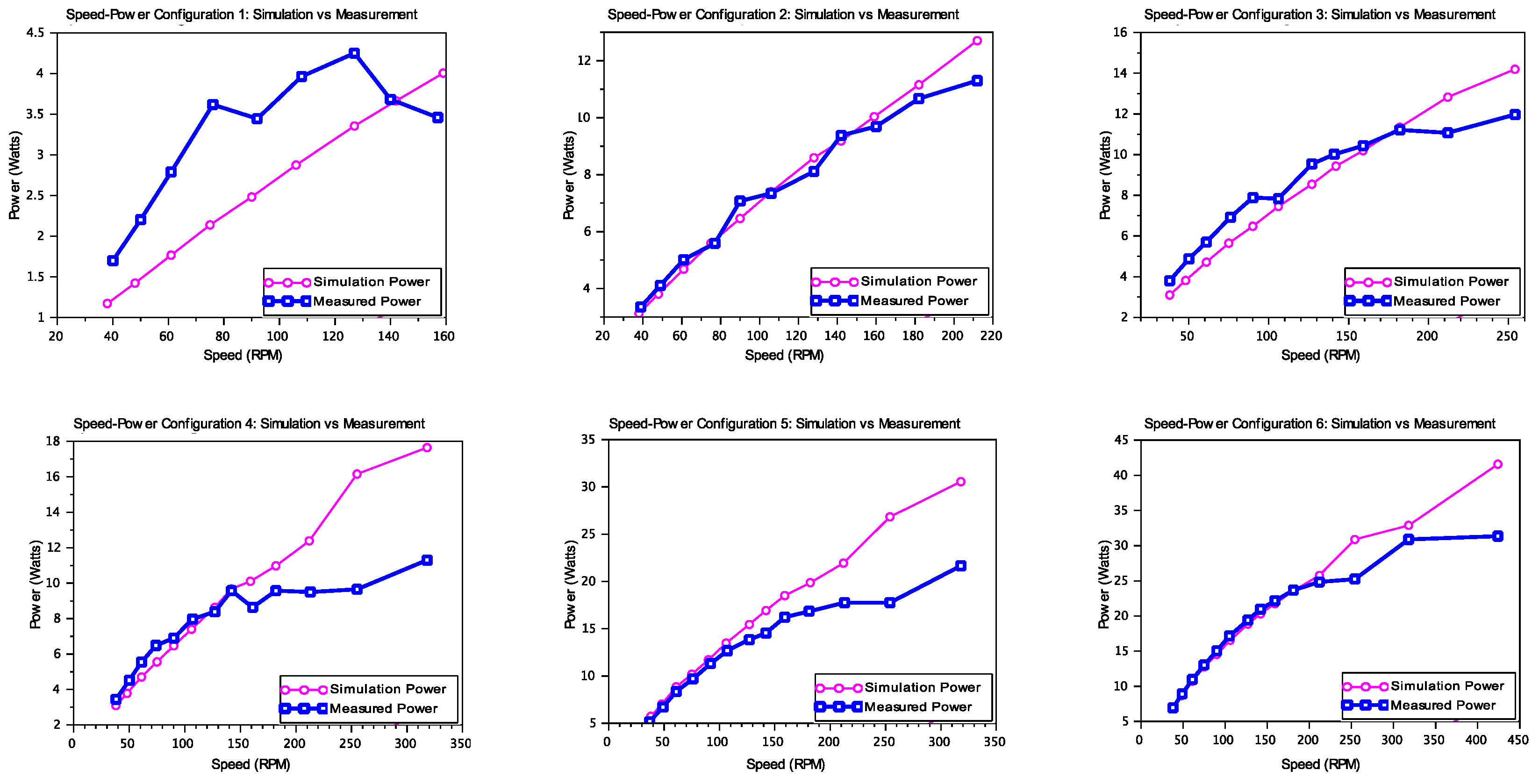
| Torque Conf. | 1 | 2 | 3 | 4 | 5 | 6 | ||||||
|---|---|---|---|---|---|---|---|---|---|---|---|---|
| Parameters | Min | Max | Min | Max | Min | Max | Min | Max | Min | Max | Min | Max |
| Simulated | 1.174 | 4.010 | 3.127 | 12.706 | 3.101 | 14.196 | 3.092 | 17.646 | 5.724 | 30.555 | 6.993 | 41.584 |
| Measured | 1.700 | 4.251 | 3.360 | 11.300 | 3.798 | 11.970 | 3.450 | 11.300 | 5.151 | 21.660 | 0.076 | 24.610 |
| % Error | 0.59 | 69.11 | 0.11 | 11.06 | 1.08 | 27.92 | 1.07 | 40.26 | 3.26 | 33.81 | 0.08 | 24.61 |
Disclaimer/Publisher’s Note: The statements, opinions and data contained in all publications are solely those of the individual author(s) and contributor(s) and not of MDPI and/or the editor(s). MDPI and/or the editor(s) disclaim responsibility for any injury to people or property resulting from any ideas, methods, instructions or products referred to in the content. |
© 2024 by the authors. Licensee MDPI, Basel, Switzerland. This article is an open access article distributed under the terms and conditions of the Creative Commons Attribution (CC BY) license (https://creativecommons.org/licenses/by/4.0/).
Share and Cite
González-Parada, A.; Moreno Del Valle, F.; Bosch-Tous, R. Design and Construction of a Multipole Electric Motor Using an Axial Flux Configuration. World Electr. Veh. J. 2024, 15, 256. https://doi.org/10.3390/wevj15060256
González-Parada A, Moreno Del Valle F, Bosch-Tous R. Design and Construction of a Multipole Electric Motor Using an Axial Flux Configuration. World Electric Vehicle Journal. 2024; 15(6):256. https://doi.org/10.3390/wevj15060256
Chicago/Turabian StyleGonzález-Parada, Adrián, Francisco Moreno Del Valle, and Ricard Bosch-Tous. 2024. "Design and Construction of a Multipole Electric Motor Using an Axial Flux Configuration" World Electric Vehicle Journal 15, no. 6: 256. https://doi.org/10.3390/wevj15060256