Path Planning Algorithms for Smart Parking: Review and Prospects

Abstract

Path planning algorithms are crucial components in the process of smart parking. At present, there are many path planning algorithms designed for smart parking. A well-designed path planning algorithm has a significant impact on the efficiency of smart parking. Firstly, this paper comprehensively describes the principles and steps of four types of path planning algorithms: the Dijkstra algorithm (including its optimized derivatives), the A* algorithm (including its optimized derivatives), the RRT (Rapidly exploring Random Trees) algorithm (including its optimized derivatives), and the BFS (Breadth First Search) algorithm. Secondly, the Dijkstra algorithm, the A* algorithm, the BFS algorithm, and the Dynamic Weighted A* algorithm were utilized to plan the paths required for the process of smart parking. During the analysis, it was found that the Dijkstra algorithm had the drawbacks of planning circuitous paths and taking too much time in the path planning for smart parking. Although the traditional A* algorithm based on the Dijkstra algorithm had greatly reduced the planning time, the effect of path planning was still unsatisfactory. The BFS (Breadth First Search) algorithm had the shortest planning time among the four algorithms, but the paths it plans were unstable and not optimal. The Dynamic Weighted A* algorithm could achieve better path planning results, and with adjustments to the weight values, this algorithm had excellent adaptability. This review provides a reference for further research on path planning algorithms in the process of smart parking.

1. Introduction

In the development of smart parking, path planning algorithms play a crucial role in ensuring the smooth operation of smart parking systems. In the context of smart parking, path planning algorithms refer to the methods that consider factors such as vehicle dimensions, parking space dimensions, and obstacle information to optimize the path for a vehicle from its current position to the target parking space. In 1959, American computer scientist Edward F. Moore first described the practical algorithm for Breadth First Search (BFS) and applied it to solving the problem of finding the shortest path in a maze (Edward F. Moore, 1959) [1]. In the same year, Dutch computer scientist Edsger W. Dijkstra proposed the Dijkstra algorithm (Edsger W. Dijkstra et al., 1959) [2]. This was one of the earliest path planning algorithms and is a greedy algorithm based on graph search. In 1968, Peter Hart, Nils Nilsson, and Bertram Raphael introduced the A* algorithm, which combines the advantages of the Dijkstra algorithm and heuristic functions, enabling it to find the shortest path from a starting point to a destination in a graph (Peter Hart et al., 1968) [3]. In 1998, Steven M. LaValle proposed the Rapidly exploring Random Tree (RRT) algorithm, which is a tree-based path planning algorithm that efficiently searches paths in high-dimensional spaces through random sampling and tree construction (Steven M. LaValle et al., 1998) [4]. In 2004, Steve Koening et al. presented the Lifelong Planning A* algorithm, which can update path planning results in real time in dynamic environments and handle global path planning offline (Steve Koening et al., 2004) [5,6]. In 2010, Dmitri Dolgov, Sebastian Thrun, and others introduced the Hybrid A* algorithm, a sampling-based path planning algorithm that can search paths in continuous spaces and handle motion constraints of vehicles and other moving objects (Dmitri Dolgov et al., 2010) [7,8]. In 2023, Honghui Fan et al. proposed the Bi-RRT^* algorithm, which introduces expanded scope, bidirectional search, and refinement in trajectory design, significantly increasing the reliability of path planning. Additionally, the inclusion of bidirectional search strategies further enhances the robustness of the paths (Honghui Fan et al., 2023) [9].

Researchers have extensively studied these algorithms and applied them specifically to the field of smart parking. The following discussion will focus on the application of various path planning algorithms in the field of intelligent parking, specifically addressing three major categories: the Dijkstra algorithm (including its optimized derivatives), the A* algorithm (including its optimized derivatives), and the RRT (Rapidly exploring Random Trees) algorithm (including its optimized derivatives).

Regarding the Dijkstra algorithm and its optimized derivatives, Jiajing Zhang et al. proposed a parking path planning algorithm based on the Dijkstra algorithm and Ant Colony algorithm to solve the problem of parking in large parking lots. They verified the superiority of the algorithm through multiple scenario experiments (Jiajing Zhang et al., 2020) [10]. Yuqing Tao used dynamic programming and the Dijkstra algorithm to develop a dynamic path planning method aiming at minimizing carbon emissions. Simulations showed that this algorithm reduces carbon emissions during the parking process to a certain extent, demonstrating great potential for low-carbon planning (Yuqing Tao, 2022) [11]. Yalin Chen improved the traditional Dijkstra algorithm by changing the data storage structure and introducing a bidirectional search strategy to plan the shortest vehicle path, thereby enhancing the path planning effect of the parking system (Yalin Chen, 2017) [12]. Zhendong Liu designed and improved the Dijkstra algorithm by reducing nodes and paths through constraint conditions and lowering computation, thereby improving parking efficiency and reducing parking costs (Zhendong Liu, 2020) [13]. Biyang Zhou et al. proposed a path planning method considering parking conflicts based on the Dijkstra algorithm. By taking road distance and average driving time as weights and introducing waiting time and travel time parameters, they set the closest distance to the elevator as the search target. Simulations showed that this path planning method can greatly reduce parking congestion problems (Biyang Zhou et al., 2021) [14]. Yanping Li et al. designed a new parking area dynamic information guidance system based on a new parking area division and parking guidance strategy. They proposed a sector area search Dijkstra algorithm that greatly alleviates congestion in the parking lot (Yanping Li et al., 2018) [15].

Regarding the A* algorithm and its optimized derivatives, Tao Gao conducted research on trajectory path planning based on the Hybrid A* algorithm, and by optimizing the heuristic function, he resolved the issue of needing to repeatedly reverse or change the driving direction in smart parking (Tao Gao, 2022) [16]. Zhang et al. proposed an optimization-based autonomous parking method. They demonstrated that the autonomous parking problem can be formulated as a smooth non-convex optimization problem. They also introduced a hierarchical Optimal Bounded Control Allocation (OBCA) algorithm, which combines the global planning capability of the Hybrid A* algorithm with the ability of OBCA to generate smooth, collision-free, and dynamically feasible paths (Zhang et al., 2018) [17]. Bailin Lu designed a self-parking path planning algorithm based on the reverse extension of the Hybrid A* algorithm. This algorithm made modifications to the node expansion logic of conventional algorithms and reduced the number of invalid path nodes by exchanging the starting and ending points of the path and expanding the path from inside the parking space (Bailin Lu, 2023) [18]. Yuan Zhang et al. addressed the issue of limited parking spaces and parking difficulties by adding a time factor to the A* algorithm, thereby designing the three-dimensional A* smart parking algorithm (Yuan Zhang et al., 2018) [19]. Sedighi et al. proposed combining the Hybrid A* algorithm with visibility graph planning to find the shortest possible non-holonomic motion-constrained path in valet parking environments (Sedighi et al., 2019) [20]. Dolgov D. et al. planned the parking path for DUC valet parking using the Hybrid A* algorithm (Dolgov D. et al., 2010) [8]. Sebastian et al. proposed an improved the Hybrid A* algorithm to plan continuous curvature paths during the parking process (Sebastian et al., 2017) [21]. Min et al. used the A* algorithm to search for parking spaces based on the predicted initial parking point, then planned the parking path with curves, achieving smart parking through multiple adjustments of the steering wheel angle (Min et al., 2015) [22]. Yutao Shi et al. proposed an efficient valet parking path planning method. For global path planning, they introduced a planner based on the Dijkstra algorithm and state lattice algorithm. For local planning, they proposed a planner based on an improved A* algorithm and Reed-Shepp curve, improving the rationality of planning paths and the efficiency of the search (Yutao Shi et al., 2022) [23]. Gaoyang Xie et al. addressed the safety issues of smart driving vehicles in uncertain environments by proposing a globally improved A* algorithm. Based on remote sensing images, they used the artificial potential field method to describe the risk distribution in uncertain environments and converted various ground conditions into travel time costs. They improved the multi-directional node search algorithm, designed a new line-of-sight algorithm, and included risk factors and travel time costs in the cost function. Simulations showed that this algorithm is well suited for path planning of smart vehicles in complex uncertain environments (Gaoyang Xie et al., 2024) [24]. Jihao Huang et al. proposed a new algorithm that integrates multi-heuristic A* algorithm and hybrid A* algorithm to solve the problem of obtaining collision-free feasible paths in a short time. This algorithm avoids local optima and generates feasible paths quickly, improving path planning efficiency (Jihao Huang et al., 2022) [25]. Yebin Wang et al. proposed a bidirectional improved A search guiding tree (BIAGT) algorithm to achieve rapid path planning by improving the node selection and node expansion of the A* algorithm. Simulations confirmed the effectiveness of this algorithm (Yebin Wang et al., 2024) [26]. Tianhao Liu et al. studied the optimization of parking trajectories for autonomous ground vehicles. To accelerate the convergence of the optimization algorithm in constrained environments, they proposed a hierarchical optimization framework. In the first layer, they designed an enhanced A* algorithm to generate reference collision-free trajectories, and in the second layer, they used gradient-based optimization with the initial guess from the first layer, considering AGV mechanical and task constraints. Simulations verified the effectiveness of the proposed solution (Tianhao Liu et al., 2022) [27]. Jiaping He et al. proposed a narrow space automatic parking path planning method. They used a fast A* algorithm to solve the discrete path points between given initial and target vehicle positions, then filtered the discrete path points to obtain “anchor points” for narrow space parking. Based on these, they generated a continuous smooth trajectory. Simulations showed that this method effectively plans paths for narrow space parking (Jiaping He et al., 2021) [28]. Weitian Sheng et al. introduced an autonomous parking trajectory planning method for narrow, unstructured environments. They proposed a multi-stage hybrid A* algorithm to handle narrow passages formed by obstacles in cluttered environments. Simulations showed that this algorithm is significantly faster than other common algorithms in handling narrow passage unstructured environments (Weitian Sheng et al., 2021) [29].

Regarding the RRT algorithm and its optimized derivatives, Long et al. designed a unified parking path planner using the Bi-RRT algorithm, which unified vertical and horizontal parking (Long et al., 2011) [30]. Kaiyu et al. used the RRT algorithm to search for constrained parking paths and then optimized the search efficiency by adopting two search strategies: target preference and Bi-RRT (Kaiyu et al., 2018) [31]. Minsoo Kim et al. combined the TargetTree-RRT^* algorithm with the optimal variant RRT to find the shortest path in smart parking path planning. Their actual experiments showed that this algorithm has higher parking accuracy, faster speed in obtaining continuous curvature paths, and a higher success rate compared to other sampling-based planning algorithms and other types of algorithms (Minsoo Kim et al., 2024) [32]. Shuang Wang et al. addressed the shortcomings of the traditional RRT algorithm, which only considers global paths in static environments and cannot avoid unknown dynamic obstacles in real-time. They proposed a path planning algorithm that integrates an improved RRT algorithm with the DWA algorithm. By introducing goal-biased random sampling and adaptive step sizes, they improved the RRT algorithm. They then used the key points of the global path generated by the improved RRT algorithm as sub-goal points for the DWA algorithm and designed an adaptive evaluation function weighting method to optimize the DWA algorithm, achieving more reasonable local path planning. Simulations demonstrated that this integrated algorithm effectively avoids dynamic obstacles (Shuang Wang et al., 2024) [33]. Yiqun Dong et al. addressed the automatic parking problem by reducing it to a path planning problem. They improved the traditional RRT algorithm by reversing its growth and using the Reed-Shepp curve to directly connect branches. They also set RRT seed biases based on parking space information. Simulations showed that this algorithm has good adaptability (Yiqun Dong et al., 2020) [34]. Qian Cheng et al. applied the asymptotically optimal Rapidly-exploring Random Tree (RRT^*) algorithm to the automatic parking scenario, calculating the optimal parking space and the driving trajectory from the current position to the optimal parking space, meeting the demand for rapid path planning in parking scenarios (Qian Cheng et al., 2023) [35]. Anand Nidhi et al. addressed the problem of parking difficulties in adverse weather conditions like rain and snow. They performed preliminary analysis of different sensors based on point cloud data and feature detection, then proposed a method using the RRT^* algorithm to achieve automatic parking of a small model car in different scenarios, based on computation time, path length, and success rate (Anand Nidhi et al., 2021) [36].

There are many existing path planning algorithms for smart parking. This paper specifically elaborates on the following categories:

(1)

Dijkstra algorithm

(2)

A* algorithm

(3)

RRT (Rapidly exploring Random Trees) algorithm

(4)

BFS (Breadth First Search) algorithm

The schematic diagram of path planning algorithm classification is shown in Figure 1.

2. Dijkstra Algorithm

As one of the earliest path planning algorithms, Dijkstra’s algorithm has played a significant role in the development of path planning algorithms [37]. This section briefly introduces the traditional Dijkstra’s algorithm and several optimized versions.

2.1. Traditional Dijkstra Algorithm

In 1959, Dutch computer scientist E. W. Dijkstra first proposed this algorithm, which is a classic shortest path algorithm 2. The basic idea is to start from the source point, greedily select a vertex with the current shortest path, and determine the shortest path of that vertex until all vertices are covered. The main feature of this algorithm is to expand outward from the starting point until the end point is reached. The basic idea of this algorithm is: Let U = (K,R) be a directed graph with weights (as shown in Figure 2), and let the set K = {0, 1, 2, 3, 4, 5}. Divide set K into two groups, the first group is set M, M = {vertices with the shortest paths already found}, initially, M only contains the source node. When a shortest path is found, the corresponding vertex is added to set M, until all vertices are added to set M; the second group is set N, N = {vertices with the shortest paths not yet determined}. During the addition process, the length of the shortest path from source node K to each vertex in set M is always less than or equal to the length of the shortest path between any two vertices in set N [38]. In Figure 2, “$5,50,10,\dots \dots$” represents the distance required to reach the specified nodes, and “$0,1,2,...,5$” represents the path nodes.

The Dijkstra algorithm is used to find the shortest path length between two vertices [38,39,40,41]. The flowchart of this algorithm is shown in Figure 3, and the specific steps are as follows:

(1)

Create a distance array to store the shortest distances from the source node to each node. Initially, set the distance from the source node to itself as 0, and distances to other nodes as infinity.

(2)

Create a set called “visit” to record the nodes with determined shortest paths.

(3)

Select the node “u” from the undetermined shortest path nodes that is closest to the source node and add it to the “visit” set.

(4)

For all neighboring nodes “v” of node “u”, if a shorter distance can be obtained through node “u”, update the shortest distance of node “v”.

(5)

Repeat steps 3 and 4 until all nodes are added to the “visit” set.

(6)

Finally, the distance array stores the shortest path lengths from the source node to other nodes.

(7)

Trace back the nodes in the “visit” set along the predecessor nodes of the shortest path until reaching the starting node, which represents the optimal planned path [42].

Ruowei Wu et al. combined the factors of path distance in the parking lot and road traffic quality and applied the Dijkstra algorithm to the parking path planning of large parking lots, helping drivers to safely and quickly complete their parking needs (Ruowei Wu et al., 2013) [43].

Shiduo Ning et al. addressed the problem of insufficient traditional parking spaces by designing a virtual smart parking system based on a signal request mechanism. They used the Dijkstra algorithm for path planning and employed the signal request mechanism to resolve deadlock conflicts, effectively solving the problem of difficult parking (Shiduo Ning et al., 2021) [44].

This algorithm can ensure the shortest path from the starting point to all other nodes, with high correctness and stability. However, the Dijkstra algorithm uses a greedy algorithm, ignoring the distribution of obstacles. Therefore, when searching in space, it will traverse all nodes, leading to a large amount of data that the algorithm needs to process. For path planning in smart parking, which requires high real-time performance, a large amount of data will increase the time cost of parking path planning [45,46,47]. Moreover, this algorithm is used to solve the single-source shortest path problem and does not consider negative weight edges [48]. Therefore, it is not suitable for path planning in images with negative weight edges because the algorithm assumes that all weight edges are non-negative. Negative weight edges will cause path planning to fail.

2.2. Bidirectional Dijkstra Algorithm

The traditional Dijkstra algorithm uses a traversal search method for full node search, which is relatively blind in the search direction and has low search efficiency. Therefore, the Bidirectional Dijkstra algorithm was introduced, which was proposed by Delling D et al. in 2009 [49]. This algorithm conducts bidirectional search in the direction, alternately from the source node and the target node, with high path search efficiency, and will provide more reasonable path planning solutions for smart parking.

The Bidirectional Dijkstra algorithm is based on the traditional Dijkstra algorithm, but it starts expanding nodes from both the start and end points simultaneously [50]. The algorithm ends when the two searches meet at the same node, and then it backtracks through the predecessor nodes to obtain the complete planned path.

Divyam Verma et al. tested the Bidirectional Dijkstra algorithm, the traditional Dijkstra algorithm, and two other algorithms in various real-world scenarios. The results showed that the Bidirectional Dijkstra algorithm was the most effective of the four algorithms in terms of time complexity, demonstrating that it could handle much larger and more complex environment maps in a very short time (Divyam Verma et al., 2021) [51].

Compared to the traditional Dijkstra algorithm, the Bidirectional Dijkstra algorithm significantly improves search efficiency by starting the search from both the start and end points simultaneously, reducing the search space and time cost [52]. However, the Bidirectional Dijkstra algorithm is more complex to implement than the traditional Dijkstra algorithm, as it needs to consider the changes in two nodes simultaneously. Also, it requires more space to store information, leading to a larger memory space requirement.

2.3. Landmark-Based Dijkstra Algorithm

The algorithm proposes the use of landmarks to accelerate the search for the shortest path, improving the traditional Dijkstra algorithm [53]. The specific steps of the algorithm are as follows:

(1)

Firstly, a set of landmarks (nodes that are representative of the graph) needs to be selected. These landmarks should be evenly distributed in the graph and should be able to represent the characteristics of the entire graph.

(2)

Then, for each pair of landmarks, the Dijkstra algorithm is used to calculate the actual distance between them. These distances are used as heuristic information to help accelerate the search for the shortest path.

(3)

Before conducting the search for the shortest path, the landmarks need to be preprocessed to calculate the shortest distance from each node to each landmark.

(4)

When it is necessary to find the shortest path from one node to another, the preprocessed information is first used to estimate the distance from the start and end points to each landmark. Combining this with the actual distance information between landmarks, the search direction is quickly determined using a heuristic method, guiding the Dijkstra algorithm to search along the most promising path.

(5)

Based on the information obtained from the Dijkstra algorithm search, the actual shortest path can be reconstructed.

This algorithm significantly improves the efficiency of the search for the shortest path by using landmarks and preprocessed information, especially for the selection of paths in complex parking environments. Additionally, this algorithm usually has a lower space complexity. However, the performance of this algorithm will vary with the choice of landmarks, which requires a certain amount of time. Also, this algorithm is more complex than the traditional Dijkstra algorithm, as it requires additional preprocessing steps.

3. A* Algorithm

The A* algorithm is a path planning algorithm that combines aspects of both low-cost-first and best-first search algorithms, using a mix of path cost and heuristic information to determine the distance of a path [54,55]. This algorithm is widely used in smart parking path planning and has several optimization variants. Here is a brief introduction to a few types of A* algorithms.

3.1. Traditional A* Algorithm

In 1968, Peter Hart et al. proposed the traditional A* algorithm [3]. The algorithm is a direct search method that is most effective for finding the shortest path in a static road network and is also an efficient algorithm for solving many search problems. The algorithm is a heuristic search algorithm that explores the state space, evaluates each search position, obtains the optimal solution, and then continues searching from this optimal solution to find the next optimal solution, until reaching the target destination. The traditional A* algorithm selects node expansion directions as shown in Figure 4.

The formula for the algorithm is represented as Equation (1).

$$f\left(n\right)=g\left(n\right)+h\left(n\right)$$

(1)

where $f\left(n\right)$ is the cost estimate from the initial state to the goal state via state $n$, $g\left(n\right)$ is the actual cost from the initial state to state $n$ in the state space, and $h\left(n\right)$ is the estimated cost of the best path from state $n$ to the goal state.

Using $d\left(n\right)$ to represent the distance from state $n$ to the goal state, the selection of $h\left(n\right)$ roughly falls into the following three cases:

If $h\left(n\right)<d\left(n\right)$, in this case, the number of search points is high, the search space is large, and efficiency is low. However, it guarantees the optimal solution.

If $h\left(n\right)=d\left(n\right)$, meaning the best path estimate $h\left(n\right)$ equals the shortest distance, then the search for paths strictly follows the shortest path, resulting in the highest search efficiency.

If $h\left(n\right)>d\left(n\right)$, the number of search points is low, the range is small, and efficiency is high, but it does not guarantee the optimal solution [56].

The specific steps of the algorithm are as follows:

(1)

Initialization:

Add the starting node to a list of nodes to be processed, initially containing only the starting node.

Set two distance values, $g\left(n\right)$ and $h\left(n\right)$, for each node. Initially, set the $g\left(n\right)$ of the starting node to 0 and the $h\left(n\right)$ to the estimated distance from the starting node to the target node.

(2)

Repeat until the target node is found or the list of nodes to be processed is empty:

Select a node with the minimum $f\left(n\right)$ value from the list of nodes to be processed as the current node. $f\left(n\right)$ is the comprehensive evaluation value defined as $f\left(n\right)=g\left(n\right)+h\left(n\right)$, where $g\left(n\right)$ is the actual distance from the starting node to the current node, and $h\left(n\right)$ is the estimated distance from the current node to the target node.

If the current node is the target node, the search ends as the shortest path is found. Otherwise, continue with the following steps.

(3)

Expand neighboring nodes:

For each neighboring node of the current node, calculate their $g\left(n\right)$ and $h\left(n\right)$ values.

If a neighboring node is not in the list of nodes to be processed, add it to the list and update its $g\left(n\right)$ and $h\left(n\right)$ values.

If a neighboring node is already in the list of nodes to be processed, check if the current path is shorter. If so, update the $g\left(n\right)$ value of the neighboring node and reset its parent node to the current node.

(4)

Repeat steps 2 and 3 until the target node is found or the list of nodes to be processed is empty.

(5)

Path reconstruction:

If the target node is found, the shortest path from the starting node to the target node can be reconstructed by backtracking through the parent nodes.

The flowchart of the algorithm is shown in Figure 5.

The algorithm has a fast response speed, capable of quickly searching possible paths [57]. However, due to the inherent constraints of its principles, it tends to have many redundant nodes, resulting in paths with multiple turns, leading to suboptimal route planning [58,59]. Additionally, the computational load for each node is significant, making the algorithm limited in handling large-scale problems [60].

3.2. Hybrid A* Algorithm

The algorithm was initially proposed by Dmitri Dolgov and Sebastian Thrun [8]. It is an enhanced A* algorithm designed for path planning on a continuous plane. It integrates discrete grid maps and continuous vehicle dynamics models and employs numerical optimization to ensure smoother planning results [61].

The search space of this algorithm is used to store information about path nodes in both continuous and discrete states. These states together form a mixed state. The continuous state must be discretized to ensure efficient searching of the cost map. The discrete state $(\tilde{x},\tilde{y},\tilde{\theta })$ is derived from the continuous state using the specific conversion formula as shown in Equation (2).

$$\begin{array}{c}\tilde{x}={\displaystyle \frac{x-O_x}{\sigma }}\\ \tilde{y}={\displaystyle \frac{y-O_y}{\sigma }}\\ \tilde{\theta }={\displaystyle \frac{\theta }{{\sigma }_{\theta }}}\end{array}$$

(2)

where $(O_x,O_y)$ is the origin of the cost map, $\sigma$ is the side length of the square grid, and ${\sigma }_{\theta }$ is the unit yaw angle for discretization.

The expansion of the node in this algorithm is achieved by extending the step size, which is a curve that must satisfy the following conditions:

(1)

In the process of expanding nodes, the number of steps in a single expansion is a positive odd number. The length of a single expansion step, denoted as $l$, must be such that it exceeds the current grid, as indicated by the condition in Equation (3).

$$l>\sqrt{2}\sigma$$

(3)

(2)

The curvature of the expansion step is constrained by the maximum steering angle of the vehicle’s front wheel, denoted as ${\delta }_{max}$, as indicated by the condition in Equation (4).

$$-{\delta }_{max}\le \delta \le {\delta }_{max}$$

(4)

(3)

The change in the steering angle of the vehicle’s front wheel, denoted as $∆\delta$ , is a multiple of the discrete unit lateral angle ${\sigma }_{\theta }$, as indicated by the condition in Equation (5).

$$∆\delta =k{\sigma }_{\theta },k\in Z$$

(5)

The accumulated cost $g\left(n\right)$ during the path planning process represents the cost from the start node to the current node, the formula as shown in Equation (6):

$$g\left(n\right)={\sum }_{i=1}^n{l}_i$$

(6)

The calculation formula for the penalty coefficient ${\lambda }_n$ in the node expansion direction during path planning is as shown in Equation (7):

$${\lambda }_n=\left\{\begin{array}{c}{c}_{forward},\mathit{Expansion}\mathit{direction}\mathit{is}\mathit{forward}\\ c_{reverse},\mathit{Expansion}\mathit{direction}\mathit{is}\mathit{backward}\end{array}\right.$$

(7)

The calculation formula for the penalty coefficient $c_n$ in the node expansion direction switch during path planning is as shown in Equation (8):

$$c_n=\left\{\begin{array}{c}0,\mathit{Expansion}\mathit{direction}\mathit{is}\mathit{the}\mathit{same}\mathit{direction}\\ c_{direction},\mathit{Expansion}\mathit{direction}\mathit{change}\end{array}\right.$$

(8)

Since the path is formed by connecting each optimal node, the selection of the optimal node is calculated and selected by the cost function $f\left(n\right)$. According to Equations (6)–(8) above, the calculation formula for the cost function $f\left(n\right)$ can be derived, which is shown in Equation (9):

$$f\left(n\right)={\lambda }_{n}g\left(n\right)+h\left(n\right)+c_n$$

(9)

where $n$ is the current node, $h\left(n\right)$ is the heuristic function, also known as the predictive cost, represents the cost from the current node to the target node.

The specific steps of the algorithm are as follows:

(1)

Initialization:

Add the starting node to a list of nodes to be processed, initially containing only the starting node.

Set two distance values, $g\left(n\right)$ and $h\left(n\right)$, for each node. Initially, set the $g\left(n\right)$ of the starting node to 0 and the $h\left(n\right)$ to the estimated distance from the starting node to the target node.

(2)

Repeat until the target node is found or the list of nodes to be processed is empty:

Select a node with the minimum $f\left(n\right)$ value from the list of nodes to be processed as the current node. $f\left(n\right)$ is the comprehensive evaluation value defined as $f\left(n\right)=g\left(n\right)+h\left(n\right)$, where $g\left(n\right)$ is the actual distance from the starting node to the current node, and $h\left(n\right)$ is the estimated distance from the current node to the target node.

If the current node is the target node, the search ends as the shortest path is found. Otherwise, continue with the following steps.

(3)

Adding the continuous vehicle dynamics model:

For a set of movements around the current position (such as straight, left turn, right turn, etc.), calculate the feasibility and cost of each movement based on the vehicle dynamics model.

For feasible movements, calculate their end positions and convert the end positions into discrete positions on the grid map.

(4)

Expanding adjacent nodes:

For each discrete position, calculate their $g\left(n\right)$ and $h\left(n\right)$ values.

If the discrete position is not in the list of nodes to be processed, add it to the list and update its $g\left(n\right)$ and $h\left(n\right)$ values.

If the discrete position is already in the list of nodes to be processed, check if the current path is shorter. If it is, update the $g\left(n\right)$ value of the discrete position and reset its parent node to the current node.

(5)

Repeat steps 2 and 4 until the target position is found or the list of nodes to be processed is empty.

(6)

Path reconstruction:

If the target position is found, a shortest path from the starting position to the target position can be reconstructed on the discrete grid map by backtracking the parent nodes. A smooth continuous motion trajectory can be generated on the path based on the control sequence of the continuous vehicle dynamics model.

Kaixiong Li et al. used the Hybrid A* algorithm to plan the path in the vertical parking of narrow parking spaces and compared with other algorithms; it was found that this algorithm could quickly plan a reasonable parking path (Kaixiong Li et al., 2023) [62].

Zhewen Tian et al. addressed the difficulty of parking semi-trailers by appropriately improving the hybrid A* algorithm to make it suitable for semi-trailer trucks. Simulation results demonstrated that the improved algorithm allowed the vehicle to accurately park in the target space (Zhewen Tian et al., 2022) [63].

Gábor G. Varga et al. designed an autonomous valet parking system, implementing the hybrid A* algorithm and RTR+CCRS planner for path planning (Gábor G. Varga et al., 2021) [64].

Zhou et al. achieved path smoothing by combining the hybrid A* algorithm with the Dual Loop-Iterative Anchoring Path Smoothing (DL-IAPS) (Zhou et al., 2021) [65].

Jixiang Su et al. proposed an optimized vertical parking path planning method based on the hybrid A* algorithm to improve the safety of automatic parking in complex environments and reduce path search time loss. They also used the Sequential Quadratic Programming (SQP) method for smoothing. Real vehicle tests showed that this method met the parking requirements in narrow spaces and had good adaptability (Jixiang Su et al., 2023) [66].

Salma M. Elshennawy et al. evaluated the uniqueness of the hybrid A* algorithm, highlighting its navigation capabilities in complex environments filled with obstacles and revealing its potential application in automatic parking systems (Salma M. Elshennawy et al., 2023) [67].

Lu Xiong et al. proposed an improved automatic parking planning algorithm for unstructured parking lot environments based on the hybrid A* algorithm. They improved the heuristic function by adding an obstacle distance penalty term on the RS curve as a heuristic item. Simulation results showed that this algorithm could be widely applied to automatic parking scenarios (Lu Xiong et al., 2021) [68].

Hyuk Oh et al. used the hybrid A* algorithm for global path planning to achieve vehicle movement from the starting position to an intermediate position. They then used clothoid-based local path planning to achieve vehicle movement from the intermediate position to the target position, realizing vertical parking path planning (In Hyuk Oh et al., 2023) [69].

This algorithm combines the continuous vehicle dynamics model, generating a smooth path while avoiding falling into local optimal solutions, effectively using heuristic functions and estimated costs, and the path search efficiency is higher. However, the disadvantage is that the complexity is higher because the vehicle dynamics model needs to be considered, and there is a discretization error, which may lead to the generated smooth path not being completely continuous on the continuous plane.

3.3. The Three-Dimensional A* Algorithm

The algorithm, based on the traditional A* algorithm, incorporates the time dimension as a criterion. If a time conflict occurs, the point is deemed unreachable, and an adjacent point that does not have a time conflict is selected. This algorithm is suitable for path planning in complex parking lots.

In order to optimize the increase in path planning computation time caused by the addition of the time criterion to the original A* algorithm, the heuristic function needs to be improved. The scale factor of the Y-axis needs to be modified so that the grid in the Y-axis direction is prioritized during path planning. The improved heuristic function is as Equation (10):

$$h\left(n\right)=\left|X_1-X_2\right|+\theta \left|Y_1-Y_2\right|$$

(10)

where $\theta$ is the scale factor of the Y-axis, in this equation, $\theta >1$. When planning a path, the algorithm will prioritize searching for empty grids in the Y-axis direction. This will reduce the cost increase caused by overlapping paths and result in a more reasonable path.

In the process of executing path planning, this algorithm initially sets the initial value of task delay to 0. Subsequently, it defines two cost vectors: $Cost\left(n\right)$ and $minCost\left(n\right)$, which are utilized to represent the cost vector and minimum cost vector, respectively. The cost vector encapsulates the expense from the origin point to the destination, distinctively encompassing both waiting time cost $W\left(n\right)$ and distance cost $D\left(n\right)$, unlike the conventional A* algorithm. Meanwhile, the minimum cost vector is defined as the result of the latest path planning cost subtracted by the previously computed path cost. When employing this algorithm for path planning, upon encountering an inaccessible parking space, it introduces a delay of one time unit before initiating the re-planning process. In the event of a feasible path being delineated, it computes the path cost along with the minimal path cost, momentarily preserving each within the $Cost\left(n\right)$ and $minCost\left(n\right)$ cost vectors. It then proceeds to introduce an additional time delay, iteratively invoking the algorithm, logging both path cost and minimal path cost on each occasion. This cycle persists until such time as the time-delay cost surpasses the minimal path cost, wherein the loop terminates, yielding the optimal path [19]. The algorithmic process is depicted in Figure 6.

In addition to the preexisting discriminants, this algorithm incorporated waiting time as a criterion, thereby significantly enhancing the efficiency of path planning. Simultaneously, it improved the operational efficiency of parking facilities and reduced parking duration. However, integrating temporal considerations increased the implementation complexity of the algorithm compared to traditional A* algorithms.

4. RRT (Rapidly Exploring Random Trees) Algorithm

The RRT algorithm, as a popular path planning algorithm, effectively addresses complex constrained path planning problems through collision detection of sampled points within the state space [70,71]. The current RRT algorithm has numerous optimized branches. The following introduces three variations of the RRT algorithm.

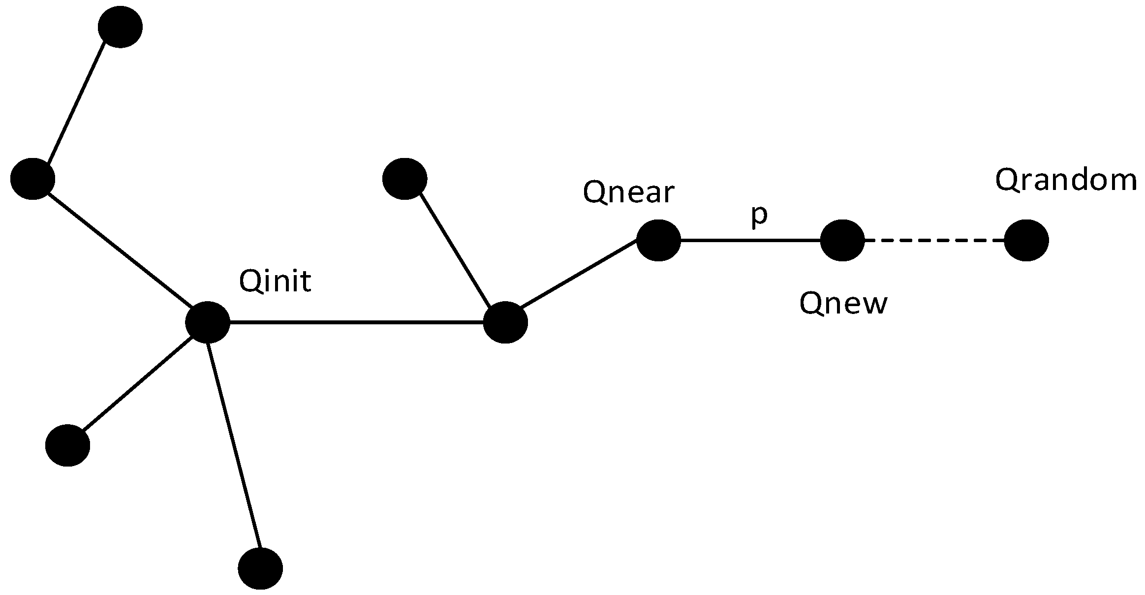
4.1. Traditional RRT Algorithm

The algorithm was first proposed by Steven M. LaValle in 1998 [72,73]. Through random sampling and rapid tree expansion, this algorithm searches for feasible paths, enabling path planning in unknown environments. The core concept involves initiating from the starting point to construct a search tree. During each iteration, a target point is randomly generated, and the node closest to this target point is selected from the search tree. This node becomes the parent node for the newly generated target point. Subsequently, the algorithm extends a certain distance along the direction of the random node to obtain a new node, repeating this process until reaching the endpoint. The schematic representation of this algorithm is illustrated in Figure 7. In Figure 7, “$Q_{init}$” represents the initial starting point, “$Q_{near}$” represents the nearest node in that situation, “$Q_{new}$” represents the newly extended node, “$Q_{random}$” represents the randomly selected point, and “$p$” represents the step size.

The specific implementation steps of the algorithm are as follows:

(1)

Initialization:

Take the starting point as the root node of the tree and add it to the initial tree.

(2)

Random Sampling:

Randomly sample points in the search space to serve as the target point. The sampling method specifics depend on the applicable environment.

(3)

Nearest Neighbor Node Selection:

Traverse all nodes in the tree to find the node closest to the randomly sampled point as the current node in the tree, using methods such as Euclidean distance to calculate the cost between nodes.

(4)

Path Extension:

Extend a certain distance from the nearest neighbor node toward the randomly sampled point to obtain a segment of the path. Other methods such as linear interpolation can be used to generate points along the path.

(5)

Collision Detection:

Perform collision detection on the points along the path to determine if they intersect with obstacles.

(6)

Connecting New Nodes:

If the path segment does not intersect with obstacles, add the endpoint of the path segment as a new node to the initial tree. Connect this new node with the nearest neighbor node to form a new tree structure.

(7)

Repeat steps 2–6 until reaching the endpoint or reaching the maximum iteration count.

(8)

After reaching the endpoint, backtrack from the endpoint along the expanded nodes to the starting point to obtain the final path.

Selim Solmaz et al. analyzed the problem of autonomous valet parking (AVP) and compared the planning performance based on the RRT algorithm. They found that this algorithm could be applied to more general low-speed autonomous environments (Selim Solmaz et al., 2021) [74].

This algorithm is an incremental approach, capable of generating paths gradually without the need to precompute the entire search space. Additionally, it performs effectively in high-dimensional spaces, exhibiting adaptability to complex and dynamically changing parking environments [75]. However, as the principle is based on random sampling, the generated paths may not necessarily be optimal. Furthermore, in the presence of numerous closely spaced obstacles, node expansion in this algorithm can be easily obstructed, leading to reduced search efficiency.

4.2. Bi-RRT (Bidirectional RRT) Algorithm

The algorithm, proposed by Steven M. LaValle in 2001, is a variant of the RRT algorithm known as Bi-RRT [76]. It employs bidirectional RRT trees to simultaneously explore the search space, aiming to find the path from the starting point to the goal. This search approach significantly reduces the search space and enhances the efficiency of finding the optimal path.

Building upon the traditional RRT algorithm, the steps of this algorithm involve simultaneously creating trees from the starting and ending points to conduct path searching. The termination condition changes such that when the most recent nodes of the two trees are within a certain distance threshold, signifying their convergence, the algorithm identifies the path. Connecting these segments yields the planned path. The schematic representation of this algorithm is illustrated in Figure 8. In Figure 8, “$Q_{start}$” and “$Q_{goal}$” represent the start and goal points, respectively; “$P_a$” and “$P_b$” represent the two nodes in bidirectional expansion; and “$P_{connect}$” represents the node that ultimately connects the two search paths.

Alex Shum et al. applied the Bi-RRT algorithm to the path planning of the rover and compared it with the bidirectional OUM. After comparing and analyzing the path planning results, they found that the Bi-RRT algorithm could handle more general weights, even negative weights, compared to the OUM. However, the Bi-RRT algorithm also had the disadvantage of slow response time and difficulty in producing the best path in a short period of time compared to the OUM (Alex Shum et al., 2015) [77].

The algorithm has good global convergence in path planning and can effectively handle sensor errors and dynamic obstacles. The solving speed has also been greatly improved compared to traditional RRT algorithms, and the convergence speed is faster. However, the algorithm also has shortcomings such as lack of heuristic information, low search efficiency, unstable path quality, slow speed in solving the optimal solution, and high computational complexity [78].

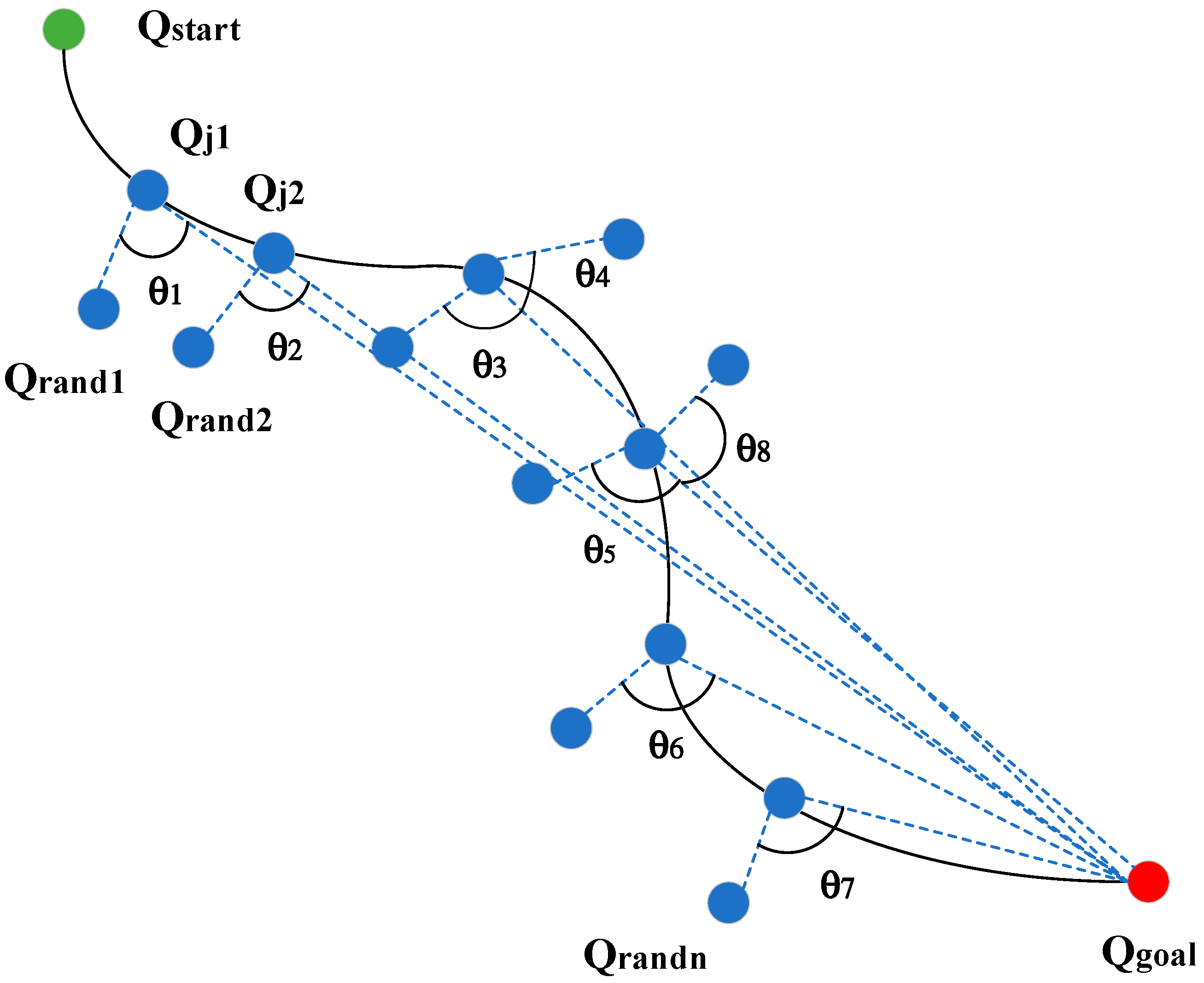
4.3. PSBi-RRT (Probabilistic Smoothed Bidirectional RRT) Algorithm

In 2022, Guojun Ma et al. proposed a new probabilistic smoothed Bi-RRT (PSBi-RRT) path planning algorithm based on bidirectional rapid search random tree (Bi-RRT), which was simulated and found to have fewer iterations as well as higher quality of path planning compared to Bi-RRT [79].

The algorithm reduces the sampling range to an ellipse based on the original Bi-RRT algorithm and uses a dual objective bias strategy for sampling, and finds the nodes near the sampling point by means of a heuristic search for neighboring points, and then evaluates the connection between two trees in both directions using the node position correction, and finally uses the $\theta -cut$ mechanism to optimize the tree.

Where the $\theta -cut$ mechanism was used to filter the redundant part of the extended nodes to improve the quality of the planned path, the filtering process of this mechanism is shown in Figure 9. In Figure 9, “$Q_{start}$” and “$Q_{goal}$” represent the start and goal points respectively, “$Q_{rand1},Q_{rand2},\dots ,Q_{randn}$” represent random nodes, and “${\theta }_1,{\theta }_2,\dots {\theta }_8$” represent the angles, which were the angle selection process of the optimization mechanism.

Compared with other RRT algorithms, the PSBi-RRT algorithm was able to adapt to the complex environment more quickly, improve the orientation of the target, and at the same time, it could well solve the problem of path zigzagging in the process of path planning, and it could also greatly reduce the loss of time and improve the efficiency of path planning in the parking process. However, the complexity of the algorithm was high, and at the same time, due to the newer algorithm, further optimization was needed.

5. BFS (Breadth First Search) Algorithm

In 1959, E.F. Moore introduced the BFS algorithm in detail and applied it to the solution of the maze problem. The Breadth First Search (BFS algorithm) is a classical graph search algorithm used to find the shortest path from the starting point to the goal node in an unweighted graph or tree.

The process of finding the shortest path in this algorithm is shown in Figure 10 with the following steps:

(1)

Initialization: mark the start node as visited point, add the start node to the queue.

(2)

Iterative process: first, take out a node from the queue as the current node, then check whether the current node is the goal node; if so, then the search ends. Conversely, if the current node is not the target node, then the neighbor nodes of the current node that have not been visited are added to the queue and they are marked as visited. When the queue is not empty, repeat the above iterative process until the target node is found.

(3)

Path backtracking: after finding the target node by backtracking nodes, so as to get the shortest path.

In Figure 10, “$Visited$” represents the traversed paths, and “$V_0,V_1,\dots V_6$” represent the path nodes.

The algorithm’s idea was simple, the implementation was relatively simple, and at the same time, it applied to the unweighted graph, which could find the required shortest path, but the algorithm may traverse a large number of nodes, which will lead to some unnecessary calculations. In addition, the node finding of the traditional BFS algorithm was incomplete, which may lead to some problems in the planned paths [80]. At the same time, for the smart parking of this kind of path planning in the presence of complex elements, it may be difficult for the BFS algorithm to meet the demand.

6. Comparison of Algorithms

In this paper, the parking environment was set to be a 500 × 500 grid, and four path planning algorithms were used to perform path planning for parking in the same environment. Figure 11 shows the time results of five runs of the four path planning algorithms, Figure 12 shows the distance results of five runs of the four path planning algorithms, Figure 13 shows the distributions of the maximum, minimum, and average values of the four path planning algorithms in terms of time; Figure 14 shows the distributions of the maximum, minimum, and average values of the four path planning algorithms in terms of distance; and

Table 1. Comparison of the four path planning algorithms.

Algorithm Type	Dijkstra Algorithm	A* Algorithm	Dynamic Weighted A* Algorithm	$\mathit{B}\mathit{F}\mathit{S}$
Average time/s	37.55646	8.51920	8.02936	6.39286
Average distance/step	926	882.4	884.6	887.8

shows the comparison of the four path planning algorithms in terms of the average time and average comparison of distances.

From the data in the above figures and tables, it can be concluded that at the level of time required to plan a path, the Dijkstra algorithm took a longer time to plan a path, which was much longer than the time required by the other three path planning algorithms. Additionally, the planning time of the Dijkstra algorithm varied greatly, leading to unstable planning times (Figure 11 and Figure 13, Table 1); the A* algorithm took a much shorter time to plan a path compared to the Dijkstra algorithm (Figure 11 and Figure 13, Table 1); The time required for path planning using the Dynamic Weighted A* algorithm was shorter compared to the A* algorithm, and the BFS algorithm required the least time among the four algorithms. (Figure 11 and Figure 13, Table 1). In terms of path planning distance, Dijkstra’s algorithm had the longest distance for five planned paths and the longest average planned distance, with average path planning stability (Figure 12 and Figure 14, Table 1). The A* algorithm had the shortest average planned distance, but its path planning stability was relatively poor, with significant variations in the planned distances (routes) (Figure 12 and Figure 14, Table 1). Although the Dynamic Weighted A* algorithm showed a slight increase in the average planned distance compared to the A* algorithm (considering that the weights in the Dynamic Weighted A* algorithm may not be the optimal choice), it had the highest stability in path planning among the four algorithms. Additionally, since the weights of the Dynamic Weighted A* algorithm could be adjusted in real time based on the map environment, it was possible to find an optimal weight that minimized both the path planning distance and time (Figure 12 and Figure 14, Table 1). The BFS algorithm resulted in an increased average distance compared to the A* and Dynamic Weighted A* algorithms, indicating that the paths planned by the BFS algorithm were not optimal. Furthermore, the stability of path planning in the BFS algorithm was poor, with significant variations (Figure 12 and Figure 14, Table 1).

The planning effects of the four algorithms were analyzed through the paths planned by the four path planning algorithms, the Dijkstra algorithm (Figure 15), the A* algorithm (Figure 16), the Dynamic Weighted A* algorithm (Figure 17), and the BFS algorithm (Figure 18).

From the four path planning diagrams, it can be seen that the paths planned by the Dijkstra and A* algorithms exhibited characteristics such as excessive winding, a high number of redundant nodes, and poor path planning efficiency. Among these, the paths generated by the Dijkstra algorithm showed greater fluctuation and longer distances compared to the A* algorithm. The paths planned by the Dynamic Weighted A* algorithm and the BFS algorithm had fewer windings and fewer redundant nodes.

Overall, the Dynamic Weighted A* algorithm had the best planning performance among the four algorithms. With its ability to adjust weights in real-time, this algorithm shows great potential for future development in path planning.

7. Summary and Prospect

7.1. Summary

Scholars have proposed the theory of different path planning algorithms; the objective of further research on path planning algorithms for smart parking is to design a robust and reliable smart parking system that can adapt to all parking environments, ensuring safe and efficient automatic parking for smart vehicles. In this paper, we have tried to select four path planning algorithms; by running the four path planning algorithms, a comparative analysis of the four path planning algorithms has been derived and summarized as follows:

(1)

The Dijkstra algorithm, the A* algorithm, the RRT algorithm, the BFS algorithm, and their respective optimization branches were discussed. The principles of these methods were described, and the advantages and disadvantages of these methods were summarized, mainly including the efficiency of path planning, the implementation difficulty of the algorithms, and the scenarios of applications.

(2)

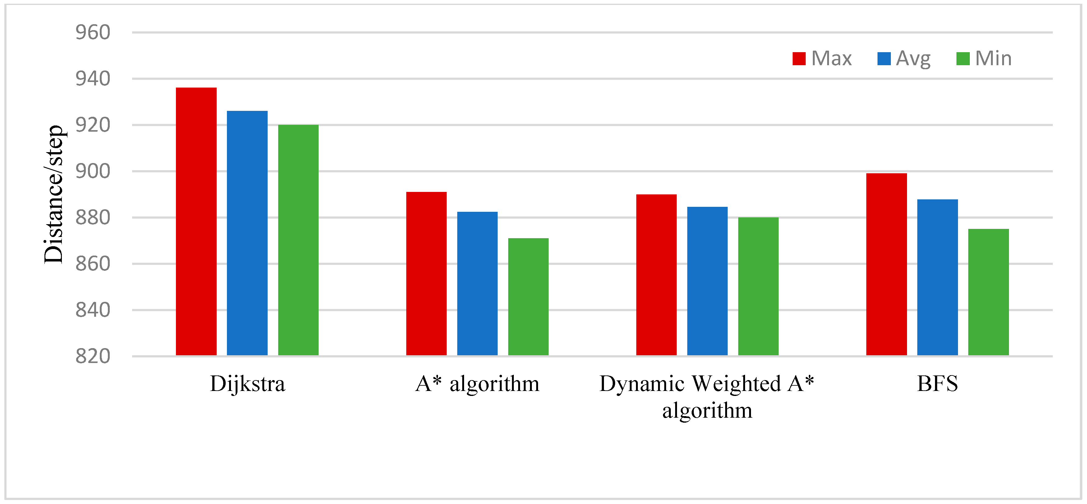
The Dijkstra algorithm was analyzed and discussed, and through comparison, it was concluded that the algorithm had a long running time, a tortuous planning path, many redundant nodes, and a long planning distance. However, the algorithm was simpler in code implementation.

(3)

The A* algorithm was analyzed and discussed, and by comparison, it was concluded that the algorithm had a shorter running time, but the planned paths were ineffective, the paths were convoluted, there was more node redundancy, and the planning distance was long.

(4)

The Dynamic Weighted A* algorithm was analyzed and discussed, and through comparison, it was found that this algorithm had a shorter running time, better planned paths, less path distortion, fewer redundant nodes, and shorter planning distances. Additionally, the weights in this algorithm could be changed in real-time, making it highly adaptable to different environments.

(5)

The BFS algorithm was analyzed and discussed, and through comparison, it was found that this algorithm had a shorter running time, generally planned paths, less path distortion, and fewer redundant nodes. However, the planned distance of this algorithm was not the optimal path.

7.2. Prospect

The current path planning algorithms still have certain limitations and need to be further studied in the following aspects:

(1)

When there are other vehicles or pedestrians moving in the parking scene, many current path planning algorithms may not be able to effectively deal with these dynamic obstacles, which may result in the planned routes not meeting the actual needs. In order to improve the effectiveness of path planning, it is necessary to improve the real-time recognition of dynamic obstacles by path planning algorithms. In environments with dynamic obstacles, the inclusion of the speed of dynamic obstacles as prior information in the path planning algorithm can help determine whether the vehicle can pass directly or needs to detour. This judgment will then guide the path planning to achieve obstacle avoidance in the presence of dynamic obstacles.

(2)

When smart parking is performed in a narrow space, the accuracy of path planning is more demanding, so the accuracy of path planning algorithms for planning paths in this parking situation needs to be improved. In narrow parking spaces, the use of higher-precision sensors can obtain more accurate environmental information. The fusion of multiple sensors can improve the accuracy of the environmental map, and improving the path planning algorithm to have more precise heuristics can be beneficial.

(3)

Different path planning algorithms have their own advantages for different parking environments, so it is a challenge to combine the advantages of these different path planning algorithms to improve the effectiveness of planning paths for various complex environments. The combination of different path planning algorithms can be based on environmental adaptation. By testing various excellent algorithms in different environments, vehicles can be equipped with different path planning algorithms tailored to specific conditions. These algorithms can then be combined for integrated path planning.

Overall, addressing the current issues in smart parking may involve improving sensor precision to ensure comprehensive and accurate obstacle information. Additionally, enhancing the accuracy of path planning algorithms and their ability to dynamically respond to various environments and obstacles could be a promising approach.

References

1. Moore, E.F. The Shortest Path Through a Maze. In Proceedings of the International Symposium on the Theory of Switching; Harvard University Press: Cambridge, MA, USA, 1959; pp. 282–295. [Google Scholar]
2. Dijkstra, E.W. A note on two problems in connexion with graphs. Numer. Mathematik 1959, 1, 269–271. [Google Scholar] [CrossRef]
3. Hart, P.E.; Nilsson, N.J.; Raphael, B. A formal Basis for the Heuristic Determination of Minimum Cost Paths. IEEE Trans. Syst. Sci. Cybern. 1968, 4, 100–107. [Google Scholar] [CrossRef]
4. LaValle, S.M. Rapidly-exploring random trees: A new tool for path planning. Res. Rep. 1998, 10, 98–111. [Google Scholar]
5. Koenig, S.; Likhachev, M.; Furcy, D. Lifelong planning A*. Artif. Intell. 2004, 155, 93–146. [Google Scholar] [CrossRef]
6. Yoon, S.; Shim, D.H. SLPA*: Shape-Aware Lifelong Planning A* for Differential Wheeled Vehicles. IEEE Trans. Intell. Transp. Syst. 2015, 16, 730–740. [Google Scholar] [CrossRef]
7. Liu, Z.; Li, Z.; Liang, K.; Yao, X.; Zhang, W. Path planning with static obstacles for USVs via the Hybrid A* algorithm and the artificial potential field method. In Proceedings of the 2022 41st Chinese Control Conference (CCC), Hefei, China, 25–27 July 2022; pp. 2894–2899. [Google Scholar]
8. Dolgov, D.; Thrun, S.; Montemerlo, M.; Diebel, J. Path planning for autonomous vehicles in unknown semi-structured environments. Int. J. Robots. Res. 2010, 29, 485–501. [Google Scholar] [CrossRef]
9. Fan, H.; Huang, J.; Huang, X.; Zhu, H.; Su, H. BI-RRT*: An improved path planning algorithm for secure and trustworthy mobile robots systems. Heliyon 2024, 10, e26403. [Google Scholar] [CrossRef] [PubMed]
10. Zhang, J.; Zhang, S.; Zhao, X.; Li, Q. An intelligent optimisation algorithm for vehicle path planning based on underground parking systems. In Proceedings of the 2020 International Conference on Intelligent Design (ICID), Xi’an, China, 11–13 December 2020; pp. 103–106. [Google Scholar]
11. Tao, Y. Dynamic Path Planning for Parking Lot Based on Carbon Emission Optimization. In Proceedings of the 2022 IEEE Conference on Telecommunications, Optics and Computer Science (TOCS), Dalian, China, 11–12 December 2022; pp. 897–902. [Google Scholar]
12. Yalin, C.; Liyang, Z.; Longbiao, Z.; Xiaojiang, S.; Heng, W. Research on path planning of parking system based on improved Dijkstra algorithm. Mod. Manuf. Eng. 2017, 443, 63. [Google Scholar]
13. Liu, Z.; Yang, Y.; Li, D.; Li, X.; Lv, X.; Chen, X. Design and Implementation of the Optimization Algorithm in the Layout of Parking Lot Guidance. In Proceedings of the 2020 16th International Conference on Computational Intelligence and Security (CIS), Guangxi, China, 27–30 November 2020; pp. 144–148. [Google Scholar]
14. Zhou, B.; Chang, Y.; Sun, C. Path optimization research based on parking conflicts in large parking lots. J. Chongqing Univ. Technol. 2021, 35, 26–33. [Google Scholar]
15. Li, Y.; Shi, B.; Wang, T.; Wang, Q.; Wu, L. Research on Intelligent Parking Area Division and Path Planning. In Advances in Internet, Data & Web Technologies, Proceedings of the 6th International Conference on Emerging Internet, Data & Web Technologies (EIDWT-2018), Tirana, Albania, 15–17 March 2018; Springer: Cham, Switzerland, 2018. [Google Scholar]
16. Tao, G. The application of intelligent vehicle parking trajectory planning. Automot. Pract. Technol. 2022, 47, 31–35. [Google Scholar]
17. Zhang, X.; Liniger, A.; Sakai, A.; Borrelli, F. Autonomous Parking Using Optimization-Based Collision Avoidance. In Proceedings of the 2018 IEEE Conference on Decision and Control (CDC), Miami, FL, USA, 17–19 December 2018; pp. 4327–4332. [Google Scholar]
18. Lu, B.L. Research on Path Planning and Tracking Control of Autonomous Parking System for Intelligent Vehicles. Master’ s Thesis, Changchun University of Technology, Changchun, China, 2023. [Google Scholar]
19. Zhang, Y.; Chen, Y.; Wei, L. Intelligent Parking Algorithm for AGV Based on Improved A* Algorithm. Comput. Syst. Appl. 2019, 28, 216–221. [Google Scholar]
20. Sedighi, S.; Nguyen, D.V.; Kuhnert, K.D. Guided hybrid A-star path planning algorithm for valet parking applications. In Proceedings of the 2019 5th International Conference on Control Automation and Robotics, Beijing, China, 19–22 April 2019; pp. 570–575. [Google Scholar]
21. Klaudt, S.; Zlocki, A.; Eckstein, L. A-priori map information and path planning for automated valet-parking. In Proceedings of the 2017 IEEE Intelligent Vehicles Symposium (IV), Redondo, CA, USA, 11–14 June 2017. [Google Scholar]
22. Min, K.W.; Choi, J.D. Design and implementation of an intelligent vehicle system for autonomous valet parking service. In Proceedings of the 2015 10th Asian Control Conference, Sabah, Malaysia, 31 May–3 June 2015; pp. 1–6. [Google Scholar]
23. Shi, Y.; Wang, P.; Wang, X. An Autonomous Valet Parking Algorithm for Path Planning and Tracking. In Proceedings of the 2022 IEEE 96th Vehicular Technology Conference (VTC2022-Fall), London, UK, 26–29 September 2022; pp. 1–7. [Google Scholar]
24. Xie, G.; Fang, L.; Su, X.; Guo, D.; Qi, Z.; Li, Y.; Che, J. A Path-Planning Approach for an Unmanned Vehicle in an Off-Road Environment Based on an Improved A* Algorithm. World Electr. Veh. J. 2024, 15, 234. [Google Scholar] [CrossRef]
25. Huang, J.; Liu, Z.; Chi, X.; Hong, F.; Su, H. Search-Based Path Planning Algorithm for Autonomous Parking: Multi-Heuristic Hybrid A*. In Proceedings of the 2022 34th Chinese Control and Decision Conference (CCDC), Hefei, China, 15–17 August 2022; pp. 6248–6253. [Google Scholar]
26. Wang, Y.; Hansen, E.; Ahn, H. Hierarchical Planning for Autonomous Parking in Dynamic Environments. IEEE Trans. Control Syst. Technol. 2024, 32, 1386–1398. [Google Scholar] [CrossRef]
27. Liu, T.; Yang, J.; Wang, W. A Hierarchical Optimization Framework for Parking Maneuver of Automated Vehicle. In Proceedings of the 2022 6th International Conference on Automation, Control and Robots (ICACR), Shanghai, China, 23–25 September 2022; pp. 156–160. [Google Scholar]
28. He, J.; Li, H. Fast A* Anchor Point based Path Planning for Narrow Space Parking. In Proceedings of the 2021 IEEE International Intelligent Transportation Systems Conference (ITSC), Indianapolis, IN, USA, 19–22 September 2021; pp. 1604–1609. [Google Scholar]
29. Sheng, W.; Li, B.; Zhong, X. Autonomous Parking Trajectory Planning with Tiny Passages: A Combination of Multistage Hybrid A-Star Algorithm and Numerical Optimal Control. IEEE Access 2021, 9, 102801–102810. [Google Scholar] [CrossRef]
30. Han, L.; Do, Q.H.; Mita, S. Unified path planner for parking an autonomous vehicle based on RRT. In Unified Path Planner for Parking an Autonomous Vehicle Based on RRT, Proceedings of the 2011 IEEE International Conference on Robotics and Automation, Shanghai, China, 9–13 May 2011; IEEE: New York, NY, USA, 2011; pp. 5622–5627. [Google Scholar]
31. Zheng, K.; Liu, S. RRT based path planning for autonomous parking of vehicle. In Proceedings of the IEEE 7th Data-Driven Control and Learning Systems Conference, Enshi, China, 25–27 May 2018; pp. 627–632. [Google Scholar]
32. Kim, M.; Ahn, J.; Park, J. TargetTree-RRT*: Continuous-Curvature Path Planning Algorithm for Autonomous Parking in Complex Environments. IEEE Trans. Autom. Sci. Eng. 2024, 21, 606–617. [Google Scholar] [CrossRef]
33. Wang, S.; Li, G.; Liu, B. Research on Unmanned Vehicle Path Planning Based on the Fusion of an Improved Rapidly Exploring Random Tree Algorithm and an Improved Dynamic Window Approach Algorithm. World Electr. Veh. J. 2024, 15, 292. [Google Scholar] [CrossRef]
34. Dong, Y.; Zhong, Y.; Hong, J. Knowledge-Biased Sampling-Based Path Planning for Automated Vehicles Parking. IEEE Access 2020, 8, 156818–156827. [Google Scholar] [CrossRef]
35. Cheng, Q.; Wang, Y. Research on Path Planning for Automatic Parking Based on RRT* Algorithm. In Proceedings of the 2023 International Conference on Advances in Electrical Engineering and Computer Applications (AEECA), Dalian, China, 18–19 August 2023; pp. 507–512. [Google Scholar]
36. Nidhi, A.; Fukuta, N. Towards Path Planning and Environmental Recognition for Autonomous Car Parking with Multiagent Control. In Proceedings of the 2021 10th International Congress on Advanced Applied Informatics (IIAI-AAI), Niigata, Japan, 11–16 July 2021; pp. 549–552. [Google Scholar]
37. Delling, D.; Goldberg, A.V.; Nowatzyk, A.; Werneck, R.F. PHAST: Hardware-accelerated shortest path trees. J. Parallel Distrib. Comput. 2013, 73, 940–952. [Google Scholar] [CrossRef]
38. Zhang, H.Y. Design and Implementation of Shortest Train Path under Emergency Events Based on Dijkstra’s Algorithm. China Storage Transp. 2023, 104–105. [Google Scholar]
39. Alyasin, A.; Abbas, E.I.; Hasan, S.D. An Efficient Optimal Path Finding for Mobile Robot Based on Dijkstra Method. In Proceedings of the 2019 4th Scientific International Conference Najaf (SICN), Al-Najef, Iraq, 29–30 April 2019; pp. 11–14. [Google Scholar]
40. Bozyiğit, A.; Alankuş, G.; Nasiboğlu, E. Public transport route planning: Modified dijkstra’s algorithm. In Proceedings of the 2017 International Conference on Computer Science and Engineering (UBMK), Antalya, Turkey, 5–8 October 2017; pp. 502–505. [Google Scholar]
41. Curtin, K.M. Network Analysis in Geographic Information Science: Review Assessment and Projections. Cartogr. Geogr. Inf. Sci. 2007, 34, 103–111. [Google Scholar] [CrossRef]
42. Jasika, N.; Alispahic, N.; Elma, A.; Ilvana, K.; Elma, L.; Nosovic, N. Dijkstra’s shortest path algorithm serial and parallel execution performance analysis. In Proceedings of the 35th International Convention, MIPRO, Opatija, Croatia, 21–25 May 2012; pp. 1811–1815. [Google Scholar]
43. Wu, R.E.; Lou, P.H. Optimal Parking Path Planning for Large Parking Lot Based on Dijkstra’s Algorithm. Ind. Control. Comput. 2013, 26, 93–95. [Google Scholar]
44. Ning, S.; Zhong, J.; Zheng, X. Design of Virtual Intelligent Parking Lot System Based on Signal Request Mechanism. In Proceedings of the 2021 IEEE 24th International Conference on Computer Supported Cooperative Work in Design (CSCWD), Dalian, China, 5–7 May 2021; pp. 593–597. [Google Scholar]
45. Yijun, Z.; Jiadong, X.; Chen, L. A Fast Bi-Directional A* Algorithm Based on Quad-Tree Decomposition and Hierarchical Map. IEEE Access 2021, 9, 102877–102885. [Google Scholar] [CrossRef]
46. Gbadamosi, O.A.; Aremu, D.R. Design of a Modified Dijkstra’s Algorithm for finding alternate routes for shortest-path problems with huge costs. In Proceedings of the 2020 International Conference in Mathematics, Computer Engineering and Computer Science (ICMCECS), Ayobo, Nigeria, 18–21 March 2020; pp. 1–6. [Google Scholar]
47. Zou, Y.M.; Yang, G.; Gao, B.Y. A path planning for robot obstacle avoidance based on Dijkstra algorithm. Math. Pract. Underst. 2013, 43, 111–118. [Google Scholar]
48. Parekh, S.; Jha, A.; Dalvi, A.; Siddavatam, I. An Exhaustive Approach Orchestrating Negative Edges for Dijkstra’s Algorithm. In Proceedings of the 2022 IEEE 7th International conference for Convergence in Technology (I2CT), Mumbai, India, 7–9 April 2022; pp. 1–5. [Google Scholar]
49. Delling, D.; Sanders, P.; Schultes, D.; Wagner, D. Engineering Route Planning Algorithms; Springer: Berlin/Heidelberg, Germany, 2009. [Google Scholar]
50. Chen, L.; Zhou, J.; Li, J.; Chen, Y. Bidirectional Dijkstra algorithm for best-routing of urban traffic network. Proc. SPIE 2007, 6754, 431–438. [Google Scholar]
51. Verma, D.; Messon, D.; Rastogi, M.; Singh, A. Comparative Study of Various Approaches Of Dijkstra Algorithm. In Proceedings of the 2021 International Conference on Computing, Communication, and Intelligent Systems (ICCCIS), Greater Noida, India, 7–9 April 2021; pp. 328–336. [Google Scholar]
52. Zhou, Z.; Wang, T.F.; Dai, G.M. Bidirectional Dijkstra binary tree algorithm for robot path planning. Comput. Eng. 2007, 33, 36–37+40. [Google Scholar]
53. Nichat, M. Landmark based shortest path detection by using Dijkestra Algorithm and Haversine Formula. Int. J. Eng. Res. Appl. 2013, 3, 162. [Google Scholar]
54. Aziz, A.; Tasfia, S.; Akhtaruzzaman, M. A Comparative Analysis among Three Different Shortest Path-finding Algorithms. In Proceedings of the 2022 3rd International Conference for Emerging Technology (INCET), Belgaum, India, 27–29 May 2022; pp. 1–4. [Google Scholar]
55. Gonçalves, S.M.M.; da Rosa, L.S.; de Marques, F.S. An Improved Heuristic Function for A∗-Based Path Search in Detailed Routing. In Proceedings of the 2019 IEEE International Symposium on Circuits and Systems (ISCAS), Sapporo, Japan, 26–29 May 2019; pp. 1–5. [Google Scholar]
56. Xu, Z.; Liu, X.; Chen, Q. Application of Improved Astar Algorithm in Global Path Planning of Unmanned Vehicles. In Proceedings of the 2019 Chinese Automation Congress (CAC), Hangzhou, China, 22–24 November 2019; pp. 2075–2080. [Google Scholar]
57. Fernandes, E.; Costa, P.; Lima, J.; Veiga, G. Towards an orientation enhanced astar algorithm for robotic navigation. In Proceedings of the 2015 IEEE International Conference on Industrial Technology (ICIT), Seville, Spain, 17–19 March 2015; pp. 3320–3325. [Google Scholar]
58. Candra, A.; Budiman, M.A.; Hartanto, K. Dijkstra’s and a-star in finding the shortest path: A tutorial. In Proceedings of the 2020 International Conference on Data Science Artificial Intelligence and Business Analytics, Medan, Indonesia, 16–17 July 2020; pp. 28–32. [Google Scholar]
59. Pan, H.; Guo, C.; Wang, Z. Research for path planning based on improved astart algorithm. In Proceedings of the 2017 4th International Conference on Information, Cybernetics and Computational Social Systems (ICCSS), Dalian, China, 24–26 July 2017; pp. 225–230. [Google Scholar]
60. Bell, B.G.H. Hyperstar: A multi-path Astar algorithm for risk averse vehicle navigation. Transp. Res. Part B Methodol. 2009, 43, 97–107. [Google Scholar] [CrossRef]
61. Ferguson, D.; Howard, T.M.; Likhachev, M. Motion planning in urban environments. J. Field Robot. 2008, 25, 939–960. [Google Scholar] [CrossRef]
62. Li, K.; Lu, J.-G.; Zhang, Q.-H. A Novel Scenario-based Path Planning Method for Narrow Parking Space. In Proceedings of the 2023 35th Chinese Control and Decision Conference (CCDC), Yichang, China, 20–22 May 2023; pp. 754–759. [Google Scholar]
63. Tian, Z.; Zhang, P.; Feng, K.; Tang, Y.; Lu, Y. Research on Vertical Parking Path Planning of Semi-trailer Train Based on Improved Hybrid A* Algorithm. In Proceedings of the 2022 2nd International Conference on Computer Science, Electronic Information Engineering and Intelligent Control Technology (CEI), Nanjing, China, 23–25 September 2022; pp. 776–780. [Google Scholar]
64. Varga, G.G.; Kondákor, A.; Antal, M. Developing an Autonomous Valet Parking System in Simulated Environment. In Proceedings of the 2021 IEEE 19th World Symposium on Applied Machine Intelligence and Informatics (SAMI), Herl’any, Slovakia, 21–23 January 2021; pp. 373–380. [Google Scholar]
65. Zhou, J.; He, R.; Wang, Y.; Jiang, S.; Zhu, Z.; Hu, J.; Luo, Q. Autonomous driving trajectory optimization with dual-loop iterative anchoring path smoothing and piecewise-jerk speed optimization. IEEE Robot. Autom. Lett. 2021, 6, 439–446. [Google Scholar] [CrossRef]
66. Su, J.; Zhang, L.; Xu, C.; He, T. Guided-TargetTree-Hybrid_A* Path Planning Algorithm for Vertical Parking. In Proceedings of the 2023 3rd International Conference on Computer Science, Electronic Information Engineering and Intelligent Control Technology (CEI), Wuhan, China, 15–17 December 2023; pp. 813–816. [Google Scholar]
67. Elshennawy, S.M.; Mohamed, O.; Mostafa, T.; Nagui, S.; Magdy, M.; Radwan, M.; Elganzory, R. Automating the Parking Process: A Study on Motion Planning Techniques for Autonomous Vehicles. In Proceedings of the 2023 Eleventh International Conference on Intelligent Computing and Information Systems (ICICIS), Cairo, Egypt, 21–23 November 2023; pp. 586–591. [Google Scholar]
68. Xiong, L.; Gao, J.; Fu, Z.; Xiao, K. Path planning for automatic parking based on improved Hybrid A* algorithm. In Proceedings of the 2021 5th CAA International Conference on Vehicular Control and Intelligence (CVCI), Tianjin, China, 29–31 October 2021; pp. 1–5. [Google Scholar]
69. Oh, I.H.; Seo, J.W.; Kim, J.S.; Chung, C.C. Reachable Set-Based Path Planning for Automated Vertical Parking System. In Proceedings of the 2023 IEEE 26th International Conference on Intelligent Transportation Systems (ITSC), Bilbao, Spain, 24–28 September 2023; pp. 1194–1200. [Google Scholar]
70. Ferguson, D.; Kalra, N.; Stentz, A. Replanning with rrts. In Proceedings of the 2006 IEEE International Conference on Robotics and Automation 2006, Orlando, FL, USA, 15–19 May 2006; pp. 1243–1248. [Google Scholar]
71. Yang, H.; Li, H.; Liu, K.; Yu, W.; Li, X. Research on path planning based on improved RRT-Connect algorithm. In Proceedings of the 2021 33rd Chinese Control and Decision Conference (CCDC), Kunming, China, 22–24 May 2021; pp. 5707–5712. [Google Scholar]
72. LaValle, S.M. Planning Algorithms; Cambridge University Press: Cambridge, UK, 2006. [Google Scholar]
73. LaValle, S.M.; Kuffner, J.J. Rapidly-exploring random trees: Progress and prospects. In Algorithmic Computer Robotics: New Directions; A K Peters: Natick, MA, USA, 2000; pp. 293–308. [Google Scholar]
74. Solmaz, S.; Muminovic, R.; Civgin, A.; Stettinger, G. Development, Analysis, and Real-life Benchmarking of RRT-based Path Planning Algorithms for Automated Valet Parking. In Proceedings of the 2021 IEEE International Intelligent Transportation Systems Conference (ITSC), Indianapolis, IN, USA, 19–22 September 2021; pp. 621–628. [Google Scholar]
75. Qiu, T.M. A Review of Motion Planning for Urban Autonomous Driving. In Proceedings of the 2023 4th International Seminar on Artificial Intelligence, Networking and Information Technology (AINIT), Nanjing, China, 16–18 June 2023; pp. 32–36. [Google Scholar]
76. Kuffner, J.J.; LaValle, S.M. RRT-connect: An efficient approach to single-query path planning. In Proceedings of the 2000 ICRA. Millennium Conference. IEEE International Conference on Robotics and Automation, San Francisco, CA, USA, 24–28 April 2000; pp. 995–1001. [Google Scholar]
77. Shum, A.; Morris, K.; Khajepour, A. Direction-dependent optimal path planning for autonomous vehicles. Robot. Auton. Syst. 2015, 70, 202–214. [Google Scholar] [CrossRef]
78. Wang, Y.; Yuan, Q.; Guo, Y.; Han, W. Path Planning for Lunar Rover Based on Bi-RRT Algorithm. In Proceedings of the 2021 40th Chinese Control Conference (CCC), Shanghai, China, 26–28 July 2021; pp. 4211–4216. [Google Scholar]
79. Ma, G.J.; Duan, Y.L.; Li, M.Z.; Xie, Z.B.; Zhu, J. A probability smoothing Bi-RRT path planning algorithm for indoor robot. Future Gener. Comput. Syst. 2023, 143, 349–360. [Google Scholar] [CrossRef]
80. Baidari, I.; Hanagawadimath, A. Traversing directed cyclic and acyclic graphs using modified BFS algorithm. In Proceedings of the 2014 Science and Information Conference, London, UK, 27–29 August 2014; pp. 175–181. [Google Scholar]
Figure 1. Path planning algorithm classification diagram.
Wevj 15 00322 g001
Figure 2. Dijkstra algorithm directed graph.
Wevj 15 00322 g002
Figure 3. Dijkstra algorithm flowchart.
Wevj 15 00322 g003
Figure 4. Node expansion directions.
Wevj 15 00322 g004
Figure 5. A* algorithm flowchart.
Wevj 15 00322 g005
Figure 6. The three-dimensional A* algorithm flowchart.
Wevj 15 00322 g006
Figure 7. RRT algorithm schematic diagram.
Wevj 15 00322 g007
Figure 8. Bi-RRT algorithm schematic diagram.
Wevj 15 00322 g008
Figure 9. θ c u t mechanism.
Wevj 15 00322 g009
Figure 10. Shortest path finding process.
Wevj 15 00322 g010
Figure 11. The time results of five runs of the four path planning algorithms.
Wevj 15 00322 g011
Figure 12. The distance results of five runs of the four path planning algorithms.
Wevj 15 00322 g012
Figure 13. The distributions of the max, min, and avg values in terms of time.
Wevj 15 00322 g013
Figure 14. The distributions of the max, min, and avg values in terms of distance.
Wevj 15 00322 g014
Figure 15. Paths planned by the Dijkstra.
Wevj 15 00322 g015
Figure 16. Paths planned by the A*.
Wevj 15 00322 g016
Figure 17. Paths planned by the Dynamic Weighted A*.
Wevj 15 00322 g017
Figure 18. Paths planned by the BFS.
Wevj 15 00322 g018