Abstract
In this paper, a time-varying delay output feedback control method based on the potential barrier function is proposed, which can solve the communication delay and field-of-view (FOV) constraints of Unmanned Ground Vehicle (UGV) clusters when communicating with ultra-wide-angle cameras. First, a second-order oscillator and an output feedback controller are utilized to feed back the position and direction of neighboring vehicles by exchanging control quantities and to solve the time-varying delay in the position computation of the ultra-wide-angle camera. Due to the limited target radiation range perceived by the camera, an FOV-constrained potential function is adopted to optimize the design of the sliding mode surface. The stability of the closed-loop control system is analyzed by applying the Lyapunov method. Finally, simulation experiments are conducted to verify the effectiveness of the consensus scheme in addressing the communication delay and FOV constraint problem under two different initial conditions.
1. Introduction
With the rapid progress in UGV technology, the applications of UGV are becoming a popular topic of discussion. Compared to a single UGV, multiple UGVs can efficiently execute complex tasks [1] to significantly enhancing the capabilities of a single UGV [2]. In practical applications, there are lots of existing ultra-wide-angle visual sensing and communication constraints. If these problems are considered, the cluster control will become more complex [3]. Therefore, it is necessary to develop a more accurate and efficient control scheme.
In the field of cluster control, UGVs are often rendezvoused to form a desired formation, which facilitates subsequent formation control. Numerous rendezvous control methods have been developed. For instance, in [4], a control formulation was proposed to ensure the control objects rendezvous by tracking the optimal trajectory. In reference [5], the rendezvous control problem was addressed by transforming it into a relaxed formulation. An effective method for generating collision-free trajectories and achieving rendezvous formation for multiple UGVs with motion constraints was demonstrated in [6]. To further improve the control accuracy and achieve the desired performance index of the closed-loop system, several studies [7,8,9,10] have applied output feedback control. In [7], only relative output measurements of neighboring agents are available to each agent. O.A.A. Orqueda et al. proposed an output feedback approach that uses a high-gain observer to estimate the derivative of the unmanned vehicles’ relative position [8]. In [9], the asymptotic output consensus result is guaranteed with the developed distributed adaptive output feedback control protocol. Reference [10] designed a cyclic-small-gain approach to distributed output-feedback control, so the outputs of the controlled agents can be driven within an arbitrarily small neighborhood of the desired agreement value under bounded external disturbances.
Additionally, the performance of a UGV cluster can be significantly affected by the continuously changing external environment. Therefore, to enable UGVs to converge into a desired formation and achieve better performance, the consensus problem has been extensively investigated. For example, Yang Liu introduces a distributed dynamic output feedback protocol that utilizes consensus control [11]. To circumvent the singularity issue, reference [12] designed an adaptive singularity avoidance fixed-time consensus control scheme. In [13], an observer-based distributed multiagent system (MAS) control scheme was proposed, which solved the consistency problem of linear multi-agent systems with input saturation and directed switching approach topologies. These methods can transform the UGV cluster into a desired geometric formation, leading to more effective control of UGVs.
Importantly, in practical applications, the information acquisition of UGVs mainly relies on the cameras [14]. However, the camera’s field of view is restricted. Without considering the FOV constraint, other UGVs or obstacles may fall outside the FOV, increasing the risk of collisions. In order to solve this problem, researchers have utilized FOV-constrained potential functions to optimize the sliding mode surface. In [15], the potential function was employed to transform the feature dynamics into equivalent dynamics with total state constraints. In [16], a three-dimensional low-order integrated guidance and control (IGC) scheme based on FOV constraint was proposed, solving the problem that the target was outside the FOV during attitude adjustment. These researchers can ensure that the target features remain within the FOV of the camera.
Due to the complexity of practical applications, the aforementioned methods typically rely on velocity sensors to estimate the control values for UGVs. Unfortunately, the system of UGV is sensitive to the failures of sensors and noise susceptibility in attitude and velocity sensors; hence, additional filters are necessary [17]. Furthermore, there is also a time delay caused by the detection and calculation of the ultra-wide-angle camera. Failure to account for these delays may prevent UGVs from performing their tasks optimally. Consequently, many researchers are devoted to overcoming these challenges [18,19,20,21]. However, the reported methods cannot transmit their coordinates to achieve consensus, which is crucial for the stability of the cluster of UGVs when the external disturbance occurs.
In this work, we present an output feedback FOV constraint consensus control to solve the rendezvous problem of UV cluster. First, based on the feedback control, the FOV constraint potential function was utilized to optimize the sliding mode surface. Then, a second-order system with virtual springs was developed to achieve the output consensus with unmeasured velocity and time delay. Finally, Lyapunov method and numerical simulations were carried out to verify the effectiveness of the proposed consensus scheme in handling communication delays and FOV constraints.
Compared with the reference mentioned above, the primary contributions of this paper are as follows:
- For the rendezvous problem of the multi-UGV cluster under the constraint of ultra-wide-angle camera sensing, the output feedback FOV constraint consensus control is proposed, which effectively improves the control accuracy of the formation;
- To address the UGV communication challenges posed by restricted viewing angles, the sliding mode surface is optimized using an FOV-constrained potential function, minimizing the risk of inter-UGV collisions;
- Aiming at the consensus problem of multiple UGV outputs with communication delays and unpredictable velocities, this paper proposes an underactuated second-order system based on virtual spring connections, aiming to enhance the formation stability of UGVs subject to external disturbances.
The rest of this article is structured as follows: in Section 2, we describe the second-order dynamic model of the UGV and introduce the main control targets. In Section 3, the Lyapunov function is applied to prove the stability of the proposed control method. In Section 4, simulation experiments are carried out to demonstrate the effectiveness of the control scheme proposed in this paper. In Section 5, the conclusion of this paper is provided.
2. Problem Description
2.1. Unmanned Ground Vehicle (UGV) Model
In this paper, a group of N unmanned ground vehicles are considered, the model of the vehicles is described as follows:
where the Equations (1) and (2) denote angular motion and linear motion, respectively. In such a model, the control inputs are the velocities and . The map is a passive map. is expressed as:
and represents the Cartesian coordinates of the vehicle, represents the orientation of the vehicle, and are the control inputs, which can be expressed as:
these inputs are defined as functions which include the torques of wheel and , the vehicle inertia I, the mass m, the radius of wheel r and the axle length of wheel R.
Remark 1.
To facilitate analysis, the angle is defined as a real variable, but this may cause unwinding that is not desired. Moreover, . The method to solve the problem of unwinding will be explained later.
2.2. Control Objective
In this part, the consensus control and the control objective are described.
The control objective in this paper is considered as a leaderless consensus problem. The coordinates and the angle rely on the initial state of UGVs and nonlinear dynamics of systems. In addition, they are not determined by a priority as a reference. As mentioned above, designing a controller that allows the vehicle to follow the leader (virtual or otherwise) while advancing in formation to solve the problem is not feasible.
In order to solve the problem of the consensus control, suppose the positioning sensors are installed in each UGV, which can provide reliable measurements of and . The UGVs are requested to converge to form a formation at a rendezvous point and obtain a common orientation . In other words, for and the vector of a UGV relative to the unknown center of the formation , the Cartesian positions are requested to converge to .
Define ; the control objective can be divided into two sub-objectives.
- (1)
- The UGV is required to join in formation near a non-predefined rendezvous point, which can be described as:
- (2)
- Each UGV has the same angular velocity and the same direction of heading; it can be described as:
2.3. FOV Constraint
2.3.1. Ultra-Wide-Angle Cameras
This paper adopts an ultra-wide-angle camera with a restricted FOV greater than 180°. The depth of field is defined by R. When such cameras are used as the only methods of sensing to collect information about other UGVs, such as position or information about the external environment, due to their inherently limited sensing or sensing capabilities, the result is limited communication capabilities for UGVs [22,23,24].
Let be the angle between the principal axis and the incoming ray. Then, when the width of FOV is greater than , satisfying the maximum incoming angle , the angle of view of the blind area is , as demonstrated in Figure 1.
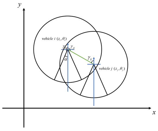
Figure 1.
Incoming angle of vehicle j to vehicle i.
If the incoming angle of the point P in a two-dimensional Cartesian coordinate system is , then the following inequation is satisfied
then point P can be detected by the camera.
The relative distance between UGV i and UGV j is . is the entry angle of UGV j relative to UGV i, so the calculation of can be expressed as
and R represent maximum viewing angle and depth of field, respectively. The visual perception topology of vehicles with FOV, which is constrained by and R, is defined as , where is the index set for all UGVs; the set of edges is denoted as .
To make i and j visible to each other, the following conditions must be satisfied
If , they can be simplified as
If each vehicle satisfies the above mutual visibility conditions, then information can be transmitted between vehicles. Due to the existence of vehicles outside the FOV constraints, the potential function is further designed to solve this problem.
2.3.2. Potential Function
Considering the ultra-wide-angle camera, the potential function will keep the vehicle within the field of view limitations through two components (angle and distance).
- (a)
- Angle-based potential functionA smooth FOV transition region is introduced; the size of the transition region is expressed by tuning parameters . Let the angle of i with respect to j be s. Therefore, the angle-based potential function can be expressed as:where ,.
- (b)
- Distance-based potential functionDesign a tuning parameter , satisfying . Then, the potential function based on distance can be expressed as:
Therefore, the potential function can be expressed as
2.4. Time Delay and Unmeasurable Velocity
The following assumptions are proposed since speed measurements are often affected by noise and sensor failures.
Assumption 1.
This paper only considers measuring coordinates and angles . Assume that the UGV can communicate with another group of UGVs through the ultra-wide-angle camera. Here, we generally believe that if the information flow is bidirectional, there is a communication connection between the two UGVs i and ; the information flow will not be lost. Therefore, the following conditions are valid.
Assumption 2.
There is a time delay from the to vehicle; namely, . Suppose the function is bounded and the second-order time derivative of the function is bounded. In addition, the upper bound of is known.
Assumption 3.
The communication of the UGV cluster can be modeled by using undirected, static and connected interconnection graphs.
Remark 2.
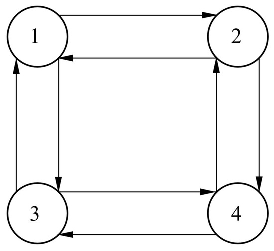
According to graph theory, a undirected graph has edges between nodes that have no direction and information can be exchanged between nodes in both directions; a static graph has connections that remain constant and if any two nodes are connected, they can be reached through other nodes. If there is a path from any vertex to another vertex, it is a connected graph, which is shown in Figure 2.
Figure 2.
Connected graph.
3. Control Design
3.1. Output Feedback Consensus Control
3.1.1. Angular Consensus
The dynamic equation (steering , and is a constant) for the consensus problem on the system can be described as:
represents the generic state and generic input. the bounded external disturbance is considered.
Based on the original proportional derivative (PD) type of distributed control law proposed in reference [24], this paper optimizes the consensus problem. By analyzing the controller of the angular motion subsystem, we can obtain:
where and . The global asymptotic stability of uniform manifolds is guaranteed.
As cannot be measured, the control law (15) cannot be adopted; we suppose that combining the second-order system with virtual springs can achieve the objective for all . The dynamic system can be described as:
where and , is an external input defined later, and the map is defined as a passive map.
In order to achieve consensus for Equation (18), if , and , a real value exists, such that for all . In addition, according to the passive map defined in Equation (1) and Equation (15), they can be combined by setting and
where is the force of torsional spring.
Theorem 1.
Based on the system Equation (1) and dynamic controller Equations (16) and (17), suppose Assumption 2 holds; the constant exists for all , , , and .
Proof of Theorem 1.
Consider the positively defined function in the consensus errors , and as follows:
where and , which is analog to the Lyapunov function. , which represents the total energy of the mass-spring system.
Taking the derivative of function (18) yields:
Then, according to the function , can be known. Based on and Equation (18), we can obtain:
Therefore, as Assumption 2 holds, the solution of this equation is for all . □
3.1.2. Position Consensus
The control law for velocity motion consensus is defined as:
Supposed the state variable is replaced by an arbitrary trajectory which is bounded and has a bounded derivative for all . Then, closed-loop linear motion dynamics can be transformed into the time-varying subsystem decoupled from angular motion dynamics, which can be described as:
where the proof of closed-loop stability of the control system is derived in Reference [3].
In order to make the position achieve the consensus point on plane , the second-order controller with a virtual-spring coupling term is used, which can be described as:
where and are the state variables of the controller; , and are control gains which are positively defined.
Then, the dynamic system (23) will be coupled with the model of the autonomous nonholonomic second-order vehicle. For the linear motion, the variation of coordinates defined by should be incorporated by the control input . Define the following function:
In order to facilitate the analysis of the control design mentioned above, the Euler–Lagrange equation is considered to simplify the consensus controller:
where and are the generalized coordinates corresponding to the links’ positions and the actuators’ angular positions, respectively. indicate Coriolis forces. is the closed-loop equation which is assimilated to the first equation in (25) with null Coriolis and gravitational forces and unitary inertia . Furthermore, when there is no significant variation in the notation, the dynamic controller (17) combined with is assimilated to the second equation of (25).
3.2. Output Feedback Consensus Control with Communication Delay
In this section, the main research result is presented: a dynamic output feedback controller designed to deal with delay measurements.
3.2.1. Main Result
In accordance with Assumption 3, the distinct measurement delays are present for each pair of UGVs. To accurately capture the influence of these delays, the consensus error is precisely expressed as follows:
For the position errors:
For the orientations:
Remark 3.
It is worth noting that the errors are defined in the coordinates of the controllers rather than the measured variables of the UGVs.
And set the communication constraints:
The angle-based potential function can be expressed as
where .
The distance-based potential function with tuning parameter can be set to satisfy condition while considering the presence of time delay. Parameter cannot be too small to ensure that the UGV remains within the FOV range within the upper bound of the time delay.
So the potential function can be expressed as:
where and . Here and are used to simplify presentation. From Equations (19) and (24), the controller that embodies the deterministic equivalence principle for the linear motion dynamics (4) is represented as follows:
for the angular motion dynamics:
Furthermore, the function has been redefined to enhance its compatibility with the output feedback controller, resulting in a more convenient formulation.
where , the function is second-order differentiable and bounded. Moreover, the derivative of the function is bounded and characterized as persistently exciting. In other words, the parameter in Equation (35) serves the same purpose as previously described. Thus, we can summarize the following information.
Proposition 1.
The system described under Assumption 1 to Assumption 3 is operated in closed-loop using the controllers given by Equations (26), (27) and (33). In this configuration, the desired goal of achieving leaderless consensus control, as defined by Equations (5) and (6), is accomplished, provided that the following condition holds:
where for all .
First, the closed-loop equations are introduced based on the method of dividing the dynamic into the linear and angular motion dynamics.
The equations obtained after calculation are as follows:
The closed-loop equations for all UGVs are represented as two interconnected dynamic feedback systems. If the state variable in Equations (40) and (41) is replaced by a fixed but arbitrary trajectory , then the above system can be viewed as an interconnected cascade configuration.
Consequently, the analysis of and can be conducted using arguments and techniques applicable to systems with a cascade configuration. In summary, it is necessary to establish the following: (1) all trajectories are bounded; (2) according to Proposition 1, for , when , the consensus error converges to zero; for , the consensus error converges due to the continuous exciting effect of . The proof is in the following two subsections.
3.2.2. Stability Proof
- (1)
- Bounded trajectories
Theorem 2.
For the system , , are all bounded and belong to . Furthermore, it is established that , indicating that the consensus error is essentially bounded. As a result, it follows that as well, signifying that the second derivative of with respect to time is also essentially bounded. Finally, it can be concluded that approaches zero or , as time progresses.
Proof of Theorem 2.
An energy-based Lyapunov–Krasovskii functional is employed, which is defined as follows:
According to Proposition 2, introducing , the function bears resemblance to an energy function; where and can be assimilated to the kinetic energy term, represents a potential energy term linked to the spring’s stiffness . in V is equivalent to .
Substituting into the derivative of yields:
Due to
where , we can obtain:
The final result can be obtained as and we know , where ,
Then, the following equation can be deduced:
where is the Laplacian matrix, and
Finally, based on the closed-loop system, the Lyapunov–Krasovskii function is obtained. The derivative of V is:
where for any , is positive.
To further analyze the trajectory behavior of , assume that . Then, there is the following Theorem. □
Theorem 3.
If , then in the trajectory of , , , and are all bounded and belong to . Finally, it can be concluded that as time progresses.
Proof of Theorem 3 is the same as Theorem 2 and we have:
In this case, , as indicated in Equation (44); is defined in a similar manner as in Equation (44), with the substitution of with and with . The derivative of the function along the trajectories of , under the condition , satisfies the following:
The positive factor of is observed in accordance with condition Equation (39). Integrating the left and right parts of the inequality in Equation (51), the first part of the Theorem can be established. Upon examining Equation (40), it becomes evident that both and are bounded and belong to . Consequently, according to Theorem 2, it can be deduced that the limit as it approaches infinity of is equal to zero; i.e., .
Proof of Theorem 3.
Similar to the function associated with the system , the function following the expression in Equation (50b) is introduced. Notably, is characterized by being positive definite and radially unbounded with respect to , and . By taking the total time-derivative of along the trajectories of Equation (37), where , the following result can be obtained:
Using the same proof method in Theorem 2 can lead to finding the total derivative of W, then Equation (41) is obtained.
According to Equation (36), there exists :
The stability proof of Equation (53) is similar to the proof of Theorem 2. It can be concluded that based on the bound in Equation (54).
where all the terms on the right are bounded; it can be deduced that the first part of the claim holds. Additionally, belongs to according to Equation (40). Consequently, it can be concluded that approaches zero; i.e., . □
Theorem 4.
With the condition of , it is correct that converges to zero,
and
It is important to note that the aforementioned statements concerning are applicable only when the condition is satisfied. If this condition is not satisfied, it should be emphasized that since , and are bounded along all trajectories, is also bounded, as indicated in Equation (33). Based on the properties mentioned, namely the boundedness of , the marginal stability of as a linear time-varying system with uniformly bounded time-delays and the resulting boundedness of , , and , it can be deduced that and are also bounded. This conclusion aligns with Proposition 3 in Reference [3].
- (2)
- Vanishing of the consensus errors
Theorem 5.
The term converges to zero asymptotically. Now, let us consider the first limit in Equation (12) and argue as follows. Given that φ is uniformly bounded, from Equation (41), it follows that belongs to and belongs to as well. Additionally, considering Assumption 3, we can infer that
This observation, along with the result that
implies, according to Barbalat’s Lemma, that . Additionally, it is worth noting that .
To understand this, consider that . As we have already shown that , it follows that as well, as required. Consequently, is uniformly continuous and tends to zero. Furthermore, from Equation (57), it also follows that approaches zero. Therefore, it can be concluded that equals zero.
Remark 4.
In a further development, it is important to highlight that and tend to zero. To understand this, consider that
Moreover, as all signals on the right side of the expression
are bounded, it can be concluded that . Consequently, is uniformly continuous and by applying Barbalat’s Lemma, it can be inferred that . Following a similar method of deriving, can be obtained.
The second limit in Equation (12) is deduced from the convergence of , and to zero (as established in Theorem 5). In fact, if , and approach zero, it follows from Equation (41) that it also converges to zero, which implies the effectiveness of the second limit in Equation (12). To gain a clearer understanding, the following equation is considered:
By defining as a vector composed of , , …, and as a vector composed of , , …, , respectively, we can express them as follows:
If and , it implies that and the existence of a vector such that or equivalently, for all .
Consequently, based on the third equation in Equation (41), it can be observed that if , and approach zero, then
and
4. Simulation
To ascertain the efficacy and stability of the ultra-wide-angle camera-based UGV consensus control, the numerical simulation experiment is conducted by using the MATLAB simulator.
4.1. Set Up
Based on reference [3], select the UGV system which is applicable for the controller designed in this paper. For convenience, the four UGVs are assumed to have the same inertia and geometric parameters, which are defined as follows:
- kg , m = 5.64 kg, r = 0.09 m and R = 0.157 m.
The information of the ultra-wide-angle camera cannot be transmitted in the process of detection and calculation, which causes communication delay. In order to simulate the time-varying delay , the random signal is adopted to follow the normal distribution, , and sample time is 10 ms. Due to the time-varying delay, the second-order system will oscillate violently or become completely unstable when the controller gain is large, so the control gain is set as follows: , , , , and .
For all , the persistent excitation function is considered as Equation (40) with . For convenience, the period functions can be described as:
where the sampling time and other parameters take the same value.
4.2. Consensus Analysis
4.2.1. Parameters of the Controller and Desired Values
In this part, a simulation experiment is conducted to verify the ability of the UGV cluster to reach the consensus state under the methodology introduced in this research paper. The control parameters and desired values are displayed in Table 1.

Table 1.
Parameters and desired values.
4.2.2. Simulation Results and Analysis
Figure 3 shows the trajectory of the rendezvous of UGVs while the initial positions are the same. Figure 4 illustrates the error of velocity and angle of UGVs. Figure 5 illustrates the control torque of the UGVs.
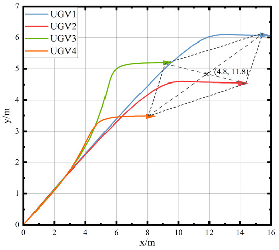
Figure 3.
Trajectory of the rendezvous diagram.
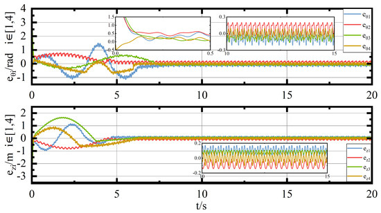
Figure 4.
Error of angle and velocity diagram.
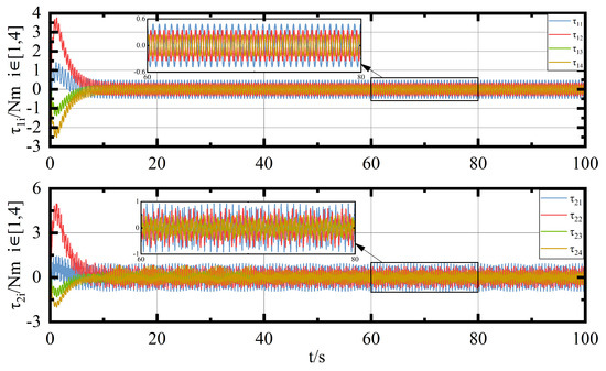
Figure 5.
Control torque diagram.
It can be seen in Figure 3 that the UGV cluster can form the desired formation, indicating that the UGV cluster reaches the consensus state in a short period, which proves that the ability to reach the consensus state is superior.
As shown in Figure 4, the speed and angle errors converges to about 0 by s, while the speed and angle errors of the UGV formation in [3] does not converge to 0 at s, which indicates that the second-order system of UGV constructed based on the virtual spring concept proposed in this paper not only enables the UGV clusters to reach a consistent state but also improves the control performance significantly.
From Figure 5, in order to maintain other UGVs and external environments within the camera’s FOV with limited observation angles, the value of the control torque will be adjusted as other UGVs get out of the FOV and basically converge to zero at s. In the reference, the control torque has not yet converged to zero at about s, This proves that the sliding mode surface designed by the FOV constraint potential function is reasonable and sufficient.
4.3. Rendezvous Control Performance and FOV Constraint Analysis
4.3.1. Parameters of the Controller and Desired Values
To validate the rendezvous performance of the UGV cluster with FOV constraint, the control parameters and desired values are shown in Table 2.
Table 2.
Parameters and desired values.
4.3.2. Simulation Results and Analysis
In this section, the simulation experiment outcomes will be shown. Figure 6 describes the trajectory of the rendezvous of UGVs while the initial positions are decentralized. Figure 7 describes the error of velocity and angle of UGVs. Figure 8 describes the control torque of the UGVs.
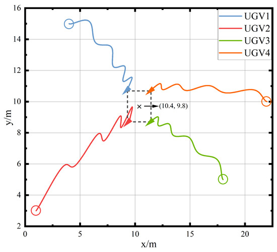
Figure 6.
Trajectory of the rendezvous diagram.
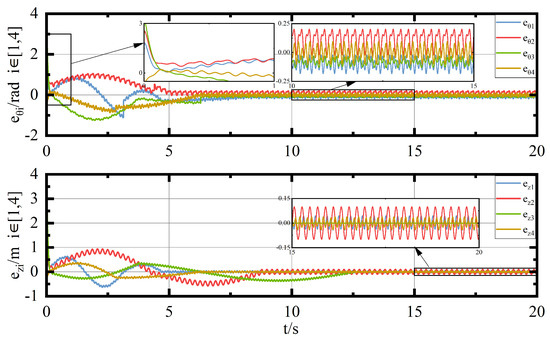
Figure 7.
Error of angle and velocity diagram.
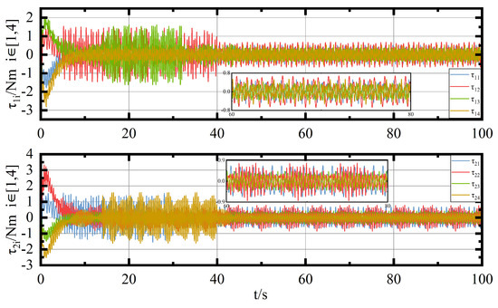
Figure 8.
Control torque diagram.
As can be seen in Figure 6, the UGVs are in their initial position; then, they rendezvous to form a desired position, whose center point is under the methodology introduced in this research paper, which indicates the effectiveness of the proposed method. Moreover, due to the influence of FOV constraints, the communication between the four UGVs is limited. The UGVs adjust output control torque to change the observation angle. Hence, the trajectory of the pre-rendezvous of UGVs is zigzag.
As can be seen in Figure 7, the fluctuation is very violent at the beginning, but it decreases gradually under the control of the proposed method. In addition, the error of angle converges to around 0 at s, while the error of velocity converges to around 0 at s. This shows that the control performance of the controller proposed in this paper is still better than the scheme in [3] under FOV constraints. Figure 8 illustrates that the control torque has strong vibration due to the influence of communication delay; after the time delay, the torque can react quickly to change the observation angle to deal with information efficiently under communication and time delay. Moreover, the control torque fluctuates within Nm at time s, indicating the UGV cluster complicates consensus and is in equilibrium. Therefore, the results prove that the proposed control scheme can maintain system dynamic equilibrium.
5. Conclusions
This paper solved the communication delay and the consensus problem of avoiding the blind area for the UGV cluster with the ultra-wide-angle camera. First, the modeling scheme of the second-order oscillator with a virtual spring could deal with the sensing delay caused by the detection and calculation of the camera, which improves the control accuracy and performance. Then, based on the modeling scheme, the FOV constraint potential function was adopted to optimize the design of the controller to avoid the control failure when the ultra-wide-angle camera is in the viewing angle blind area, thus avoiding the serious adverse consequences of collision between different UGVs. In addition, the Lyapunov method was applied to analyze the stability of a closed-loop control system. Finally, the simulation results showed that the proposed control scheme could effectively reach the consensus state and complete the rendezvous task, which could be widely adopted in practical engineering applications.
Author Contributions
Conceptualization, L.L. and Y.W.; methodology, L.L.; software, L.L. and Y.W.; validation, W.S. and C.X.; formal analysis, W.S. and L.L.; investigation and resources, L.L.; data curation, C.X.; writing—original draft preparation, Y.W.; writing—review and editing, Y.W.; visualization, W.S.; supervision, C.X.; project administration, W.S. All authors have read and agreed to the published version of the manuscript.
Funding
This research received no external funding.
Data Availability Statement
The data that support the findings of this study are available from the corresponding author upon reasonable request.
Conflicts of Interest
Chao Xiong and Wei Shang are employees of Ningbo Cixing Co., Ltd. The paper reflects the views of the scientist and not necessarily those of the company.
References
- Arafat, M.Y.; Moh, S. A survey on cluster-based routing protocols for unmanned aerial vehicle networks. IEEE Access 2018, 7, 498–516. [Google Scholar] [CrossRef]
- Li, J.; Zhao, M.; Ding, Y.; Liu, D.Y.; Wang, Y.; Liang, H. An aggregate authentication framework for unmanned aerial vehicle cluster network. In Proceedings of the 2020 IEEE nternational Conference on Parallel and Distributed Processing with Applications, Big Data and Cloud Computing, Sustainable Computing and Communications, Social Computing and Networking (ISPA/BDCloud/SocialCom/SustainCom), Exeter, UK, 17–19 December 2020; pp. 1249–1256. [Google Scholar]
- Nuno, E.; Loria, A.; Panteley, E.; Restrepo, E. Rendezvous of nonholonomic robots via output-feedback control under time-varying delays. IEEE Trans. Control. Syst. Technol. 2022, 30, 2707–2716. [Google Scholar] [CrossRef]
- Rucco, A.; Sujit, P.B.; Aguiar, A.P.; De Sousa, J.B.; Pereira, F.L. Optimal rendezvous trajectory for unmanned aerial-ground vehicles. IEEE Trans. Aerosp. Electron. Syst. 2017, 54, 834–847. [Google Scholar] [CrossRef]
- Lu, P.; Liu, X. Autonomous trajectory planning for rendezvous and proximity operations by conic optimization. J. Guid. Control. Dyn. 2013, 36, 375–389. [Google Scholar] [CrossRef]
- Chandra, R.S.; Breheny, S.H.; D’Andrea, R. Antenna array synthesis with clusters of unmanned aerial vehicles. Automatica 2008, 44, 1976–1984. [Google Scholar] [CrossRef]
- Dong, S.; Chen, G.; Liu, M.; Wu, Z.-G. Intermittent Cluster Consensus Control of Multiagent Systems From a Static/Dynamic Output Approach. IEEE Trans. Syst. Man Cybern. Syst. 2022, 52, 7727–7736. [Google Scholar] [CrossRef]
- Orqueda, O.A.A.; Zhang, X.T.; Fierro, R. An output feedback nonlinear decentralized controller for unmanned vehicle co-ordination. Int. J. Robust Nonlinear Control. IFAC-Affil. J. 2007, 17, 1106–1128. [Google Scholar] [CrossRef]
- Hua, C.; Cui, R.; Ning, P.; Luo, X. Event-Based Output Feedback Consensus Control for Multiagent Systems with Unknown Non-Identical Control Directions. IEEE Trans. Circuits Syst. I Regul. Pap. 2023, 70, 1747–1757. [Google Scholar] [CrossRef]
- Liu, T.; Jiang, Z.-P. Distributed Output-Feedback Control of Nonlinear Multi-Agent Systems. IEEE Trans. Autom. Control. 2013, 58, 2912–2917. [Google Scholar] [CrossRef]
- Liu, Y.; Jia, Y.; Du, J.; Yuan, S. Dynamic output feedback control for consensus of multi-agent systems: An H∞ approach. In Proceedings of the 2009 American Control Conference, St. Louis, MO, USA, 10–12 June 2009; pp. 4470–4475. [Google Scholar]
- Su, Y.; Xue, H.; Liang, H.; Chen, D. Singularity avoidance adaptive output-feedback fixed-time consensus control for multiple autonomous underwater vehicles subject to nonlinearities. Int. J. Robust Nonlinear Control. 2022, 32, 4401–4421. [Google Scholar] [CrossRef]
- Fan, M.C.; Zhang, H.T.; Lin, Z. Distributed semiglobal consensus with relative output feedback and input saturation under directed switching networks. IEEE Trans. Circuits Syst. II Express Briefs 2015, 62, 796–800. [Google Scholar] [CrossRef]
- Li, X.; Tan, Y.; Tang, J.; Chen, X. Task-Driven Formation of Nonholonomic Vehicles with Communication Constraints. IEEE Trans. Control. Syst. Technol. 2022, 31, 442–450. [Google Scholar] [CrossRef]
- Salehi, I.; Rotithor, G.; Saltus, R.; Dani, A.P. Constrained image-based visual servoing using potential functions. In Proceedings of the 2021 IEEE International Conference on Robotics and Automation (ICRA), Xi’an, China, 30 May–5 June 2021; pp. 14254–14260. [Google Scholar]
- Zhang, D.; Ma, P.; Du, Y.; Chao, T. Integral barrier Lyapunov function-based three-dimensional low-order integrated guidance and control design with seeker’s field-of-view constraint. Aerosp. Sci. Technol. 2021, 116, 106886. [Google Scholar] [CrossRef]
- Nuno, E. Consensus of Euler–Lagrange systems using only position measurements. IEEE Trans. Control. Netw. Syst. 2016, 5, 489–498. [Google Scholar] [CrossRef]
- Lee, J.; Yoo, C.; Park, Y.S.; Park, B.; Lee, S.J.; Gweon, D.G.; Chang, P.H. An experimental study on time delay control of actuation system of tilt rotor unmanned aerial vehicle. Mechatronics 2012, 22, 184–194. [Google Scholar] [CrossRef]
- Armah, S.K.; Yi, S. Analysis of Time Delays in Quadrotor Systems and Design of Control. In Time Delay Systems. Advances in Delays and Dynamics; Insperger, T., Ersal, T., Orosz, G., Eds.; Springer: Cham, Switzerland, 2017; Volume 7. [Google Scholar] [CrossRef]
- Abdessameud, A.; Tayebi, A. Formation control of VTOL unmanned aerial vehicles with communication delays. Automatica 2011, 47, 2383–2394. [Google Scholar] [CrossRef]
- Zhang, X.; Zhou, D.; Zhang, J.; Pan, Q.; Zhang, K. Based on backstepping control with time-delay estimation and nonlinear damping adaptive PID control for unmanned aerial vehicle. In Proceedings of the 2015 IEEE International Conference on Information and Automation, Lijiang, China, 8–10 August 2015; pp. 1310–1315. [Google Scholar] [CrossRef]
- Roelofsen, S.; Martinoli, A.; Gillet, D. Distributed deconfliction algorithm for unmanned aerial vehicles with limited range and field of view sensors. In Proceedings of the 2015 American Control Conference (ACC), Chicago, IL, USA, 1–3 July 2015; pp. 4356–4361. [Google Scholar]
- Roelofsen, S.; Martinoli, A.; Gillet, D. 3D collision avoidance algorithm for unmanned aerial vehicles with limited field of view constraints. In Proceedings of the 2016 IEEE 55th Conference on Decision and Control (CDC), Las Vegas, NV, USA, 12–14 December 2016; pp. 2555–2560. [Google Scholar]
- Ren, W.; Beard, R.W. Distributed Consensus in Multi-Vehicle Cooperative Control; Springer: London, UK, 2008. [Google Scholar]
Disclaimer/Publisher’s Note: The statements, opinions and data contained in all publications are solely those of the individual author(s) and contributor(s) and not of MDPI and/or the editor(s). MDPI and/or the editor(s) disclaim responsibility for any injury to people or property resulting from any ideas, methods, instructions or products referred to in the content. |
© 2024 by the authors. Licensee MDPI, Basel, Switzerland. This article is an open access article distributed under the terms and conditions of the Creative Commons Attribution (CC BY) license (https://creativecommons.org/licenses/by/4.0/).