Energy-Aware 3D Path Planning by Autonomous Ground Vehicle in Wireless Sensor Networks

Abstract

Wireless sensor networks are used to monitor the environment, to detect anomalies or any other problems and risks in the system. If used in the transportation network, they can monitor traffic and detect traffic risks. In wireless sensor networks, energy constraints must be handled to enable continuous environmental monitoring and surveillance data gathering and communication. Energy-aware path planning of autonomous ground vehicle charging for sensor nodes can solve energy and battery replacement problems. This paper uses the Nearest Neighbour algorithm for the energy-aware path planning problem with an autonomous ground vehicle. Path planning simulations show that the Nearest Neighbour algorithm converges faster and produces a better solution than the genetic algorithm. We offer robust and energy-efficient path planning algorithms to swiftly collect sensor data with less energy, allowing the monitoring system to respond faster to anomalies. Positioning communicating sensors closer minimizes their energy usage and improves the network lifetime. This study also considers the scenario in which it is recommended to avoid taking direct travelling pathways between particular node pairs for a variety of different reasons. To address this more challenging scenario, we provide an Obstacle-Avoided Nearest Neighbour-based approach that has been adapted from the Nearest Neighbour approach. Within the context of this technique, the direct paths that connect the nodes are restricted. Even in this case, the Obstacle-Avoided Nearest Neighbour-based approach achieves almost the same performance as the the Neighbour-based approach.

1. Introduction

Wireless sensor networks (WSNs) are crucial for data collecting, resource exploration, and navigation due to their rapid development [1]. Contrary to conventional networks, a Wireless Sensor Network (WSN) possesses a distinctive architecture and constraints on the resources it can access. Resource limits include a limited communication range, a finite energy supply from a battery, restricted bandwidth, and a confined CPU and storage capacity that cannot handle complex control algorithms. Optimising communication in Wireless Sensor Networks (WSNs) is critical for minimising energy utilization due to the short battery life of sensor nodes and the high energy consumption of data transmission [2]. In WSNs, a key goal is to provide efficient and reliable wireless connectivity to maximize the network’s longevity [3].

There exist several research studies on gathering data with a static sink to reduce total energy consumption in a WSN [4,5,6]. On the other hand, gathering data with a mobile sink reduces energy consumption more in WSNs; therefore, path planning of a mobile sink is an important problem in WSNs. The proposed metaheuristic-based path planning strategy for a WSN expedites sensor data collection while conserving energy, enabling a faster monitoring system reaction to accident hazards. Positioning communicating sensors closer minimizes their energy consumption. This increases the lifespan of a WSN, which monitors the environment to detect anomalies and prevent accidents.

Several studies have tackled 3D path planning problems in underwater wireless sensor networks (UWSNs) similar to the 3D path planning problem tackled in this paper. Firstly, WSNs need massive amounts of energy for data transmission. Sensory data are compressed and optimized for reducing energy consumption and transmission [7]. Second, clever node placement and routing can boost UWSN energy efficiency. Through the optimization of deployment and routing operations, it is possible to decrease the amount of energy that is consumed and to increase network lifetime. This is due to variation in the distance between data sensor nodes as well as the amount of energy that is expended between them [8].

Even with these approaches, changing the battery when it dies is required. Underwater sensors can be charged using energy transfer technologies for long-term monitoring and transmitting data without the need for battery replacement [9]. The work [10] developed a rechargeable lithium-ion battery module for underwater use, addressing high water pressure and short circuits. Due to energy transfer distance limitations, autonomous underwater vehicles need help charging and require route planning.

An Autonomous Underwater Vehicle (AUV) is a self-propelled submarine capable of moderate activities without human intervention [11]. AUVs are widely used in undersea study, environmental monitoring, and marine safety because of their affordability and security in seabed inquiry, search, identification, and rescue [12]. The AUV’s limited power-carrying capacity and charging area make data loss from its consecutive nodes problematic. This makes it difficult to guarantee the AUV’s usefulness for broader detecting regions, especially in marine conditions.

Magnetically charged cars for wireless rechargeable sensor networks (WRSNs) were proposed in [13]. In ground-based wireless rechargeable sensor networks, WSNs have a three-dimensional structure and improve transmission power with distance.

In this paper, we focus on the path planning problem in both cases without an obstacle and with an obstacle, which is where the difficulty of our problem comes from. On the other hand, we assume perfect accuracy to hit the sensor nodes.

The most significant contributions are summarized in the following, which is a shortened version:

• This paper consider the energy-aware path planning problem with an automated guided vehicle (AGV) in a 3D environment different from most of the related literature.
• This research gives a comparative study of three commonly used approaches for three-dimensional path planning by an AGV. The discussion focuses on the challenges that arise while collecting data in wireless sensor networks.
• We propose the Nearest Neighbour (NN)-based approach as a method that can be utilized in the real world to solve the three-dimensional path planning problem. This method considers the computing limitations that emerge during the process.
• A modified version of the Nearest Neighbour algorithm, the Obstacle-Avoided Nearest Neighbour (OANN)-based approach, is proposed as a solution for avoiding obstacles to the three-dimensional path planning problem. The travelling constraints occurring between particular sensor pairs are considered whenever this strategy is utilized.

The rest of the paper will follow this format. Section 2 briefly describes related studies in the literature. In Section 3, the problem is defined and its system model is given. In Section 4, various methods for solving the 3D path planning problem are presented. In Section 5, we present a novel approach by considering the problem with some limitations between some of the sensor pairs. We evaluate the proposed approaches’ performance in Section 6. Section 7 concludes the paper and gives the future work.

2. Related Work

This section considers the related literature to effectively tackle path planning in a WSN.

The limitations of batteries necessitate the development of alternatives to communication methods that conserve energy. Lee et al. studied network topology-based energy-efficient WSN MAC techniques [14]. In [15], energy-efficient and reliable WSN MAC and routing algorithms are examined. Ref. [16] introduces a packet-sending method to improve channel quality and decrease redundancy. Su et al. [17] have created a hybrid-coding-aware routing solution that is applicable to the realm of underwater acoustic sensor networks (UASNs). This strategy reduces the amount of transmission overhead while also enhancing dependability.

Clustering improves lifespan, resource management, data aggregation, and energy efficiency in wireless sensor networks [18]. The network is divided into clusters, each with a cluster head (CH) relaying information to reduce redundant transfers [19]. Energy and bandwidth savings exist in challenging fields with limited communication resources [20].

In the work [21], a clustering-based communication protocol lowered sensor node energy usage. Jin et al.’s topology management solution improves coverage and longevity, ensuring reliable connectivity [22]. Ref. [23] presented a virtual force-based distributed node deployment strategy to improve WSN network coverage. A network topology control model in [24] optimizes data transmission and extends network lifespan for features such as robustness, energy consumption balance, and topology.

AGVs charge, collecting data as the UAV gathers data. Sensor-equipped AGVs can collect geology, water quality, and marine life data. In [25], AGV-assisted communication was tested, with the AGV gathering energy-saving data as a mobile node. In [26], AGVs were proposed for data collecting and K-means pathway planning [27]. AGVs are used for data collection and multi-hop detection [28].

AGVs or central stations can receive data from mobile or stationary sensors. We can coordinate the activities live. Kan et al.’s [29] field-deployable three-phase wireless charging system charges AGVs quickly and easily. According to the work in [30], using dynamic system theory for AGV navigation in 0–100 m depths led to faster battery life.

Building autonomous-docking, battery-charging AGVs allows long-term operation without human intervention. The dock charges sensor nodes and AGV batteries. Their efficiency and independence increase without retrieval and recharge.

Efficiency is improved via AGV path design. Cheng et al. apply kinematic and dynamical models to plan AGV routes, avoid obstacles, and assess energy usage for energy savings and network longevity [31]. Kumar and colleagues [32] propose a hybrid underwater AGV exploration technique that considerably restricts their range. In [33], the exploring region is separated into smaller parts with data collecting points. Prepared pathways conserve AGV energy when gathering data. A rechargeable method [34] extends network life.

A path planning and energy-saving technique for using AUVs can handle the network energy limits and battery replacement issues ([35]). While many AUVs charge sensor network nodes, a genetic algorithm selects the optimal path to maximize network size and transmission reliability. The simulation demonstrates that while energy balancing node density and network size, the AUV path planning method converges more quickly than the conventional approaches and lengthens the lifetime of WSNs. In high-density networks, our path planning saves 15% of the energy used by exploratory AUVs.

Autonomous ground vehicles have attracted a lot of attention as workable solutions for a variety of military and civilian applications. However, in challenging circumstances (e.g., border enforcement and planetary exploration) where they must operate autonomously with limited onboard power, energy consumption plays a crucial role in autonomous ground vehicle navigation. It is expected that under these circumstances, autonomous ground vehicles will be able to perform more tasks more efficiently while using less electricity. While most studies have created an effective methodology for designing dynamically feasible and energy-efficient trajectories for skid steering or differential steering vehicles, there are few studies known on path planning for Ackermann steering autonomous ground vehicles. The paper [36] presents a completeness-guaranteed, energy-efficient path planning technique for autonomous ground vehicles with Ackermann steering, based on the $A^{*}$ search algorithm. The energy cost model of the autonomous ground vehicle is initially built using its kinematic constraints. Next, given the start and target states, the energy cost model is utilized to build the energy-aware motion primitives offline and calculate the cost of each primary trajectory. Lastly, a completeness property analysis is presented along with a proposal for an energy-efficient path planner. The effectiveness of the proposed energy-efficient journey planner is validated by means of simulation on over 150 randomly generated maps and real car testing. The results show that a small departure from the distance-optimal path can save energy expenses by around 26.9% in simulation and 21.09% in an actual test scenario for autonomous ground vehicles with Ackermann steering.

In the paper [37], the Nearest Neighbour algorithm is used to solve the energy-aware path planning problem associated with an Autonomous Underwater Vehicle (AUV). The simulations indicate that the Nearest Neighbour approach achieves faster convergence and produces superior solutions in comparison to the Genetic Algorithm and Grey Wolf Optimizer algorithm. They facilitate rapid gathering of sensor data while minimising energy usage.

The paper [38] employs the closest neighbour technique to solve the energy-aware path planning problem of an autonomous underwater vehicle. Path planning simulations indicate that the Nearest Neighbour technique achieves faster convergence and produces superior results when compared to the genetic algorithm. They successfully collect sensor data while minimising energy usage. This allows the monitoring system to quickly discover and respond to anomalies. This study also considers scenarios in which it is recommended to avoid selecting direct travel routes between certain pairs of nodes for various reasons. A modified Nearest Neighbour-based approach is proposed to address this challenging scenario. The direct connections between these nodes are restricted in situations where the modified version of the Nearest Neighbour-based technique shows significant effectiveness.

Most papers dealing the energy-aware path planning problem with an AGV consider the problem in a 2D environment. On the other hand, the vehicles can face mounds or even small hills, which can even cause altitude difference. Therefore, we consider the energy-aware path planning problem with an AGV in a 3D environment.

3. System Model and Problem Definition

Our study addresses the energy-aware path planning problem for an AGV’s sensor visit. We provide a motivating scenario and define this problem accordingly. First, we examine the UWSN system model. The path planning problem is then defined more clearly.

3.1. System Model

Refer to Figure 1 for the network model. Every sensor node sends data to the cluster head node via a wireless network. Magnetic resonance coupling AGVs charge each sensor node before returning to a charge station (CS) to rest and for data collection.

The energy consumption balance of sensors is an important problem for WSNs. In various research studies [39,40,41], AGVs collect data to handle the problem of unequal energy use. The AGV visits each sensor node according to a strategy to balance energy usage.

3.2. Problem Definition

The problem of energy-aware path planning through the use of an AGV is classified as the travelling salesman problem (TSP) [39,40,41]. Classical search algorithms and evolutionary algorithms are two primary approaches that are usually utilized in the process of resolving the TSP. The artificial potential field approach, greedy algorithm, and quick progress algorithm are all examples of algorithms that fall within the previously mentioned category. Methods such as biological algorithms like the Genetic Algorithm, Grey Wolf Optimizer algorithm and Nearest Neighbour algorithm are included in the latter category.

The most prominent NP-hard optimization problem is the TSP [40,41]. The TSP algorithm generates an optimized itinerary for a salesman, starting from their house, visiting multiple places, and returning with the minimum travel time, ensuring that each city is visited only once [42].

In a TSP problem with m sensor nodes, let $c_{ij}$ be the node distance from node i to node j. Indicate by $x_{ij}$ a binary variable that assumes the value of 1 if node j is visited right after node i. If neither of them exist, it uses 0. In this case, the energy-aware path planning problem can be seen as an NP-hard TSP in the way that follows [43]:

Problem 1.

Minimizing the following cost function:

$${\displaystyle \underset{x_{ij}}{min}\sum _{j=1}^m\sum _{i=1}^m{c}_{ij}{x}_{ij}}$$

(1)

where

$$\begin{array}{ccc}\hfill \sum _{i=1}^m{x}_{ij}& =& 1,j=1,\dots ,m\hfill \\ \hfill \sum _{j=1}^m{x}_{ij}& =& 1,i=1,\dots ,m\hfill \\ \hfill \sum _{i\in K}\sum _{j\in K}{x}_{ij}& \le & \left|K\right|-1,\forall K\subset \{1,\dots ,m\}\hfill \end{array}$$

4. Proposed Energy-Aware Path Planning (EAPP) Approaches

This section deals with the energy-aware path planning problem of an automated guided vehicle (AGV). The distance between every two sensor node pairs is the issue at hand. The most famous NP-hard optimization problem is thought to be the TSP [40,41]. With multiple visits to each city, the TSP can create a route for a salesman that starts at his house, visits several locations, and then returns to the starting point with the least amount of travel time [42].

In the energy-aware path planning problem, most of the studies use the metaheuristic or approximation algorithms. Therefore, we use these commonly used algorithms for the comparative study in this section. Some other works propose different algorithms for different scenarios; however, they are not applicable for the TSP-type path planning problem investigated in this paper.

The genetic algorithm is known as an efficient metaheuristic for the TSP problem so it is applied to the TSP problem at hand. On the other hand, as a recently proposed technique in 2014, the Grey Wolf algorithm is also considered for the TSP problem at hand. Finally, as an approximation algorithm, the Nearest Neighbour algorithm is applied to this problem because it is much faster and more robust than the metaheuristic techniques. Therefore, we consider the problem with an obstacle avoidance issue by using the Nearest Neighbour algorithm, which shows the best performance among all the three algorithms.

By tackling the EAPP problem as a TSP problem, we present a Nearest Neighbour (NN)-based approach, Grey Wolf Optimizer (GWO)-based approach, and Genetic Algorithm (GA)-based approach.

4.1. Nearest Neighbour (NN)-Based Approach

At the same time that we present a solution that is based on the Nearest Neighbour algorithm [44], we address the EAPP problem as a TSP.

4.2. Grey Wolf Optimizer (GWO)-Based Approach

Our methodology entails tackling the EAPP problem as a TSP and implementing a solution for 3D path planning that is based on the Grey Wolf Optimizer algorithm [45]. To do this, we have developed a solution.

4.3. Genetic Algorithm (GA)-Based Approach

In order to address the EAPP problem, which we address as a TSP, we present a solution that is based on the genetic algorithm and is a three-dimensional path planning solution [46,47]. The primary concept behind genetic algorithms is to attempt to solve tough optimization problems by modelling their behaviour after that of biological evolution. This is carried out in an effort to solve optimal problems. In order to address TSP difficulties, the process of using a genetic algorithm begins with the identification of the people that comprise the TSP solution and the initialization of the population. These are the beginning steps of the process. In the process of selecting individuals for various genetic processes like selection, crossover, and mutation in the population, each individual can be evaluated based on a fitness function. Individuals who are thought to be the most fit are selected. The maximum number of iterations that have been selected is the final criterion that will help determine whether or not the GA will be terminated. Regarding this study, the individual fitness is defined by the total route size or the total energy consumption of the AGV. Both of these factors are taken into consideration.

4.4. Computational Complexity

This section investigates the computational complexity of the NN-based approach, GA-based approach and GWO-based approach.

4.4.1. Computational Complexity of NN-Based Approach

Given a fixed dimension, a semi-definite positive norm (which includes every $L^p$ norm), and n points in this space, the Nearest Neighbour of each point may be found in $O\left(nlogn\right)$ time. In $O\left(mnlogn\right)$ time, the m Nearest Neighbours of each point may be located, where n is the number of nodes to be visited in our problem.

4.4.2. Computational Complexity of GA-Based Approach

The computational complexity of the GA-based approach is $O\left(n^2\right)$ since it uses nested loops for calculating the fitness value of each individual in the population, where n is the number of nodes to be visited in our problem.

4.4.3. Computational Complexity of GWO-Based Approach

The computational complexity of the GWO-based approach is $O\left(n^2\right)$ of $O(N\times m)$ time, where N represents the population size and m represents the dimension of the problem. Given a maximum number of iterations, the total time complexity of the DGWO and GWO is $O(N\times m\times MaxIter)$, where $MaxIter$ indicates the maximum number of iterations.

5. Obstacle-Avoided Nearest Neighbour (OANN)-Based Approach

The problem of energy-aware path planning is tackled in this section, which also takes into account the constraints that are imposed by some sensor pairs because of their proximity to one another. When there are obstacles situated between sensors, there is a possibility that they will hinder the direct movement of data from one sensor to the other. The autonomous ground vehicle (AGV) does not wish to travel directly from one sensor to the second sensor for a variety of reasons. Each of these reasons is discussed in more detail below. They include potentially hazardous objects, routes that are limited or muddy between the two sensors, and temperatures that are constantly changing. Within the context of this particular situation, the AGV will make its way to a sensor or sensors that are situated in the middle of the two sensors.

A modified version of the Nearest Neighbour algorithm, which we refer to as the Obstacle-Avoided Nearest Neighbour (OANN)-based approach, is what we propose as a solution to the problem of three-dimensional path planning. This strategy aims to address minuscule obstructions that frequently develop in the space between some sensor pairs.

$$D=\left[\begin{array}{ccccc}{d}_{11}& d_{12}& \dots & d_{1n}& d_{1n}\\ d_{21}& d_{22}& \dots & d_{1n}& d_{1n}\\ ⋮& ⋮& \ddots & ⋮& ⋮\\ d_{(n-1)1}& d_{(n-1)2}& \dots & d_{(n-1)(n-1)}& d_{(n-1)n}\\ d_{n1}& d_{n2}& \dots & d_{n(n-1)}& d_{nn}\end{array}\right].$$

(2)

If travelling from node $(n-1)$ to node n is impossible due to obstacles or some other blockage, then $d_{(n-1)n}=M$, where M is a very large number.

By giving a large number M such that $d_{(n-1)n}=d_{n(n-1)}=M$, the modified distance cost matrix $D_{mod}^{OA}$ obtained before using the Nearest Neighbour approach for n nodes is

$$D_{mod}^{OA}=\left[\begin{array}{ccccc}{d}_{11}& M& \dots & d_{1n}& d_{1n}\\ M& d_{22}& \dots & d_{1n}& d_{1n}\\ ⋮& ⋮& \ddots & ⋮& ⋮\\ d_{(n-1)1}& d_{(n-1)2}& \dots & d_{(n-1)(n-1)}& M\\ d_{n1}& d_{n2}& \dots & M& d_{nn}\end{array}\right].$$

(3)

By considering this modified distance cost matrix $D_{mod}^{prac}$, we use a 3D Nearest Neighbour algorithm. Hence, we proposed the Obstacle-Avoided Nearest Neighbour (OANN)-based approach, which has the same computational complexity as the Nearest Neighbour-based approach.

6. Numerical Results

This section compares the effectiveness of algorithms used for the 3D energy-aware path planning problem of an autonomous ground vehicle (AGV). The factor that is taken into consideration is the distance that exists between every pair of sensor nodes. Through the process of randomly placing sensor nodes, we were able to establish a region that was 500 m by 500 m by 500 m so that we could carry out the simulations. Similar works chose a range of dimension lengths and distances that were equivalent to the strategy that we used.

In the energy-aware path planning problem, most of the studies use the metaheuristic or approximation algorithms. Therefore, we use these commonly used algorithms for the comparative study in this section. There are some other works which propose different algorithms for different scenarios which are not applicable in our scenarios.

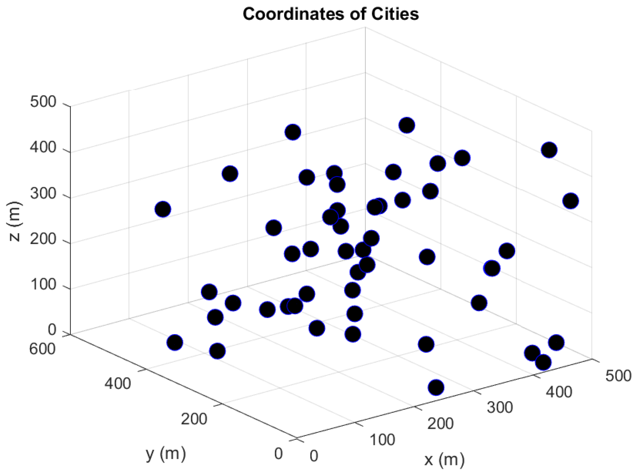
6.1. 50-Node Scenario

This subsection evaluates the proposed algorithms numerically for a scenario with a single AGV and 50 nodes. Figure 2 illustrates 50 nodes located in a 500 m × 500 m × 500 m space.

In Figure 2, we generate the locations of 50 nodes by considering uniform random distribution for them. The locations of the 50 nodes are given as {(441, 21, 473), (501, 58, 326), (284, 290, 66), (293, 310, 107), (56, 148, 389), (453, 21, 46), (237, 382, 179), (424, 10, 17), (158, 462, 37), (76, 29, 451), (142, 73, 154), (291, 355, 347), (3, 214, 112), (147, 178, 126), (157, 208, 284), (448, 262, 361), (107, 140, 229), (449, 483, 171), (427, 111, 222), (488, 280, 22), (258, 241, 185), (324, 161, 226), (140, 21, 385), (295, 107, 401), (413, 354, 410), (438, 61, 13), (240, 6, 28), (257, 271, 220), (318, 389, 243), (208, 298, 389), (168, 155, 442), (149, 464, 95), (186, 104, 279), (271, 446, 27), (347, 262, 304), (388, 233, 381), (398, 415, 212), (30, 369, 62), (151, 119, 370), (206, 66, 490), (117, 351, 125), (224, 360, 459), (459, 202, 138), (14, 99, 243), (339, 187, 19), (59, 446, 315), (429, 153, 167), (213, 157, 282), (209, 331, 94), (101, 334, 421)}.

With different subsets of these parameters, we evaluate performance of the Nearest Neighbour (NN)-, Grey Wolf Optimizer (GWO)-, and Genetic Algorithm (GA)-based approaches.

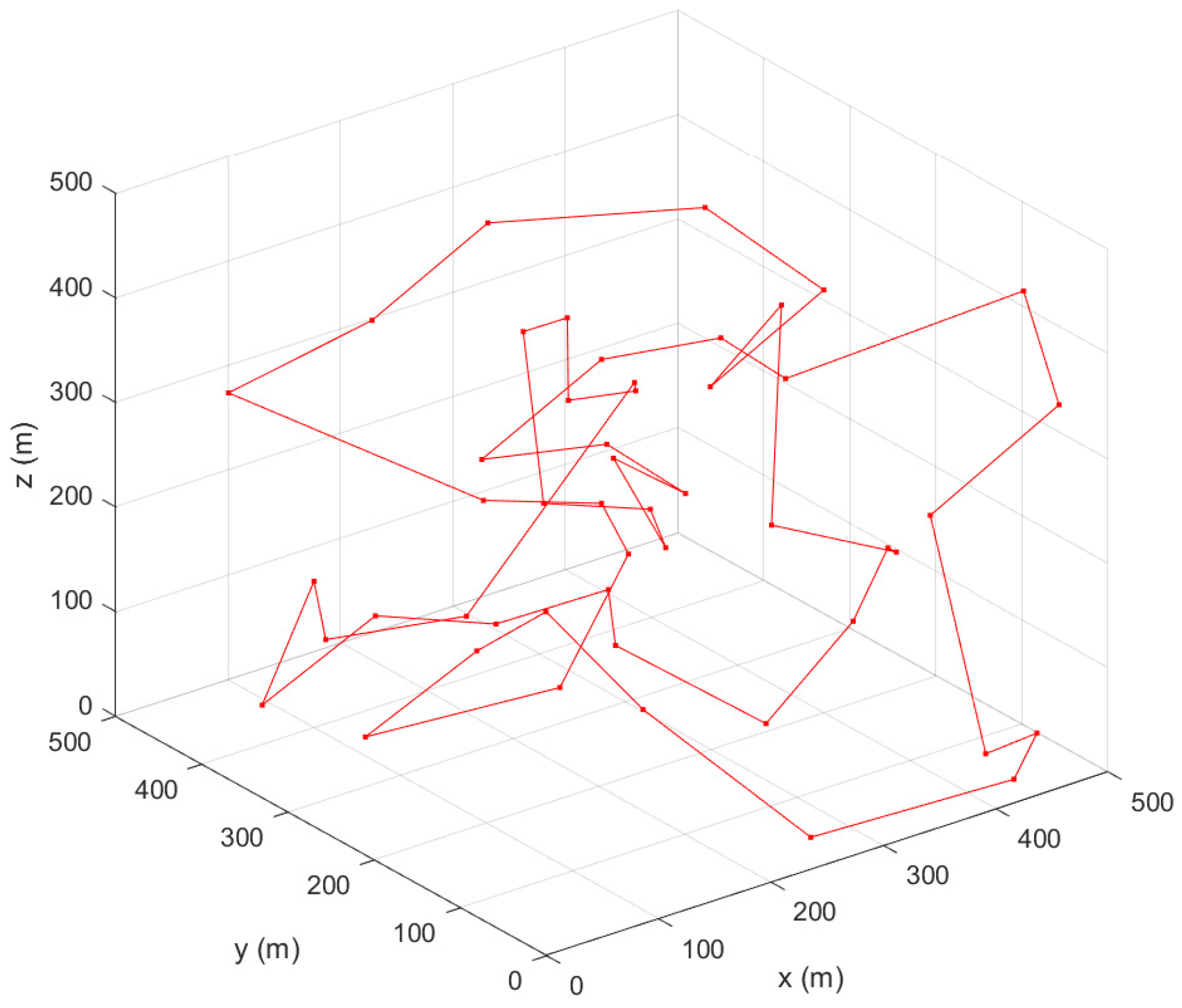
6.1.1. NN-Based Approach

This subsection evaluates the performance of an NN-based solution. Figure 3 demonstrates the NN’s achieved path planning solution in the scenario in Figure 2.

In Figure 3, the NN-based approach achieves a path length of 6358 m (please note that as an approximation algorithm, it is not an iterative algorithm).

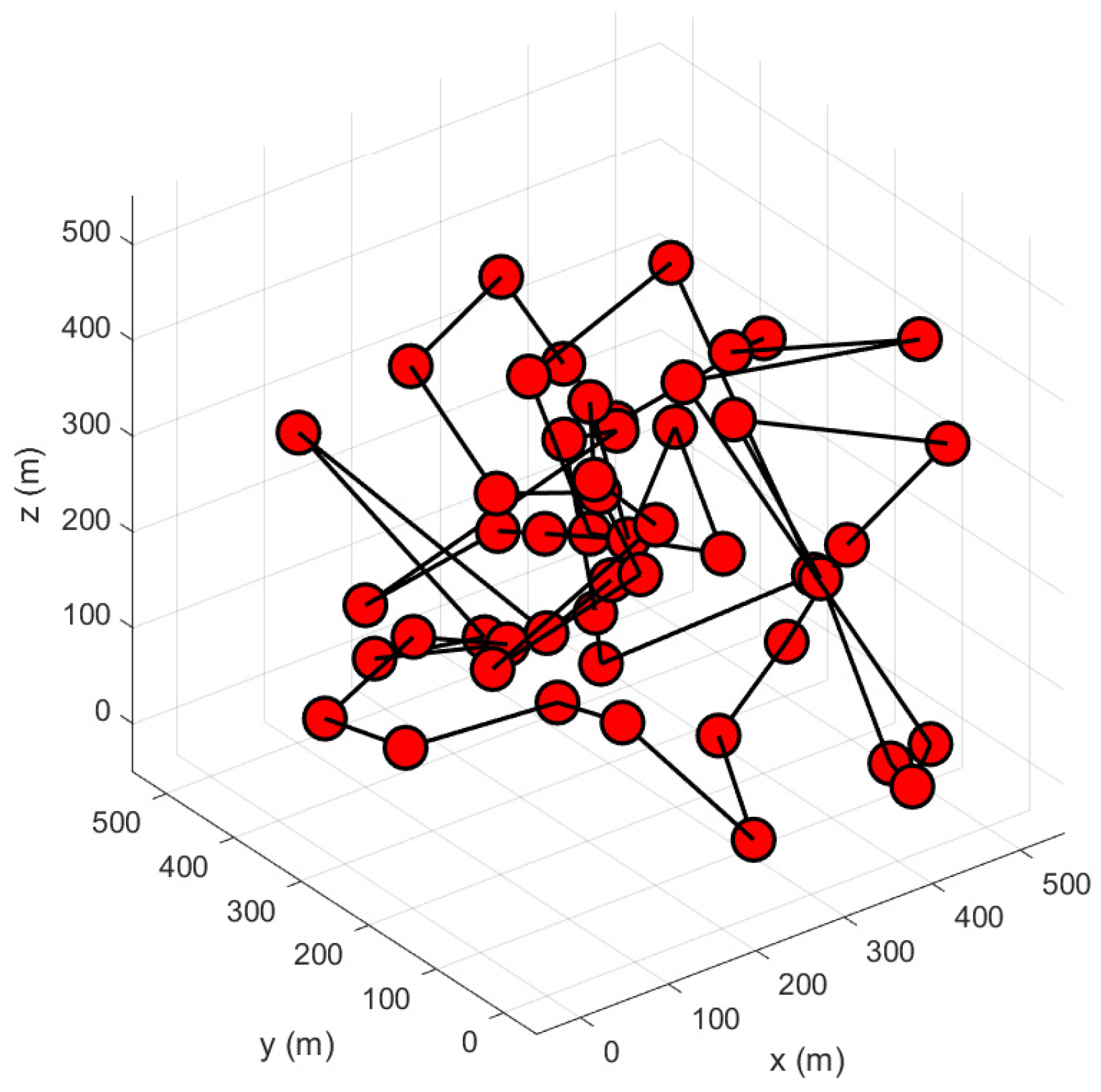
6.1.2. GA-Based Approach

This subsection evaluates performance of a GA-based solution. Figure 4 demonstrates the GA’s achieved path planning solution in 1000 iterations in the scenario in Figure 2.

In Figure 4, the GA-based approach achieves a path length of 6227 m in 1000 iterations as a metaheuristic which approaches the solution iteratively.

6.1.3. GWO-Based Approach

This subsection evaluates performance of a GWO-based solution. Figure 5 demonstrates the GWO’s achieved path planning solution in 1000 iterations in the scenario in Figure 2.

In Figure 5, the GWO-based approach achieves a path length of 8837 m in 1000 iterations as a metaheuristic which approaches the solution iteratively.

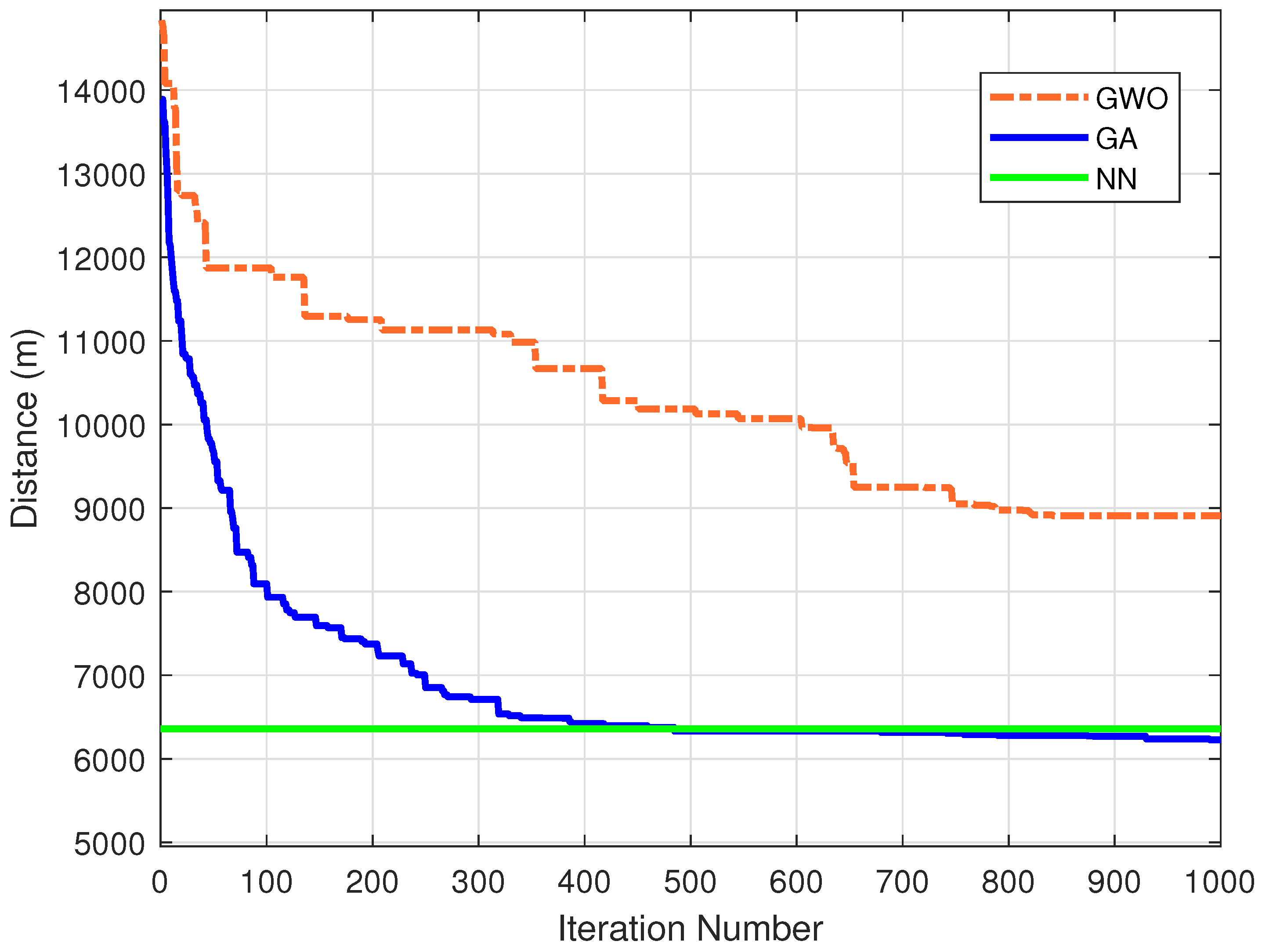
6.1.4. Comparison and Discussion

In general, the NN-based approach achieves a better performance than the GA-based approach.

Figure 6 shows the total distance travelled by the AGV with different algorithms (NN-based approach, GWO-based approach, and GA-based approach) to visit the 50 sensor nodes given in Figure 2.

From Figure 6, the following observations can be made for the performance of the algorithms for the 50-node scenario. Considering the general trend, the NN-based approach and the GA-based approach perform better than the GWO-based approach. Not only does the NN-based approach give better results than the GA-based approach until the 500th iteration, but the NN-based approach also solves in a much shorter time (0.098977 s) compared to the GA-based approach’s time to reach the solution (3.689545 s). The NN-based approach performs 37.4 times faster than the GA-based approach.

From

Table 1. Total path length (in terms of meters) to visit 50 nodes with NN-, GWO-, and GA-based approaches with respect to iteration number.

Iter.	100	200	300	400	500	600	700	800	900	1000
GWO	11,874	11,254	11,130	10,669	10,186	9996	9251	8977	8837	8837
GA	8094	7374	6712	6420	6330	6330	6314	6279	6271	6227
NN	6358	6358	6358	6358	6358	6358	6358	6358	6358	6358

, we can make the following observations. In the first iteration, the GA-based approach and GWO-based approach started with high values of path lengths (14,000–15,000 m), while the NN-based approach achieved a solution of around 6360 m very quickly. At the 100th iteration, the GA-based approach achieves significantly better results than the GWO-based approach (3000 m, i.e., 32% shorter path than that achieved by the GWO-based approach). At the 300th iteration, the NN-based approach achieves better results than the GWO- and GA-based approaches. At the 600th iteration, the GA-based approach achieves better results than the NN-based approach. At iteration 1000, the GA-based approach significantly outperforms the GWO-based approach (2610 m, i.e., 29.5% less than the GWO-based approach), while achieving a shorter path than the NN-based approach; the NN-based approach provides a much faster and practical solution.

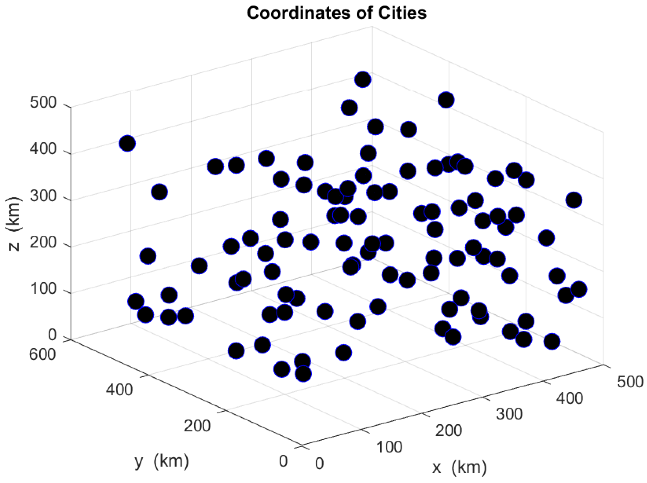
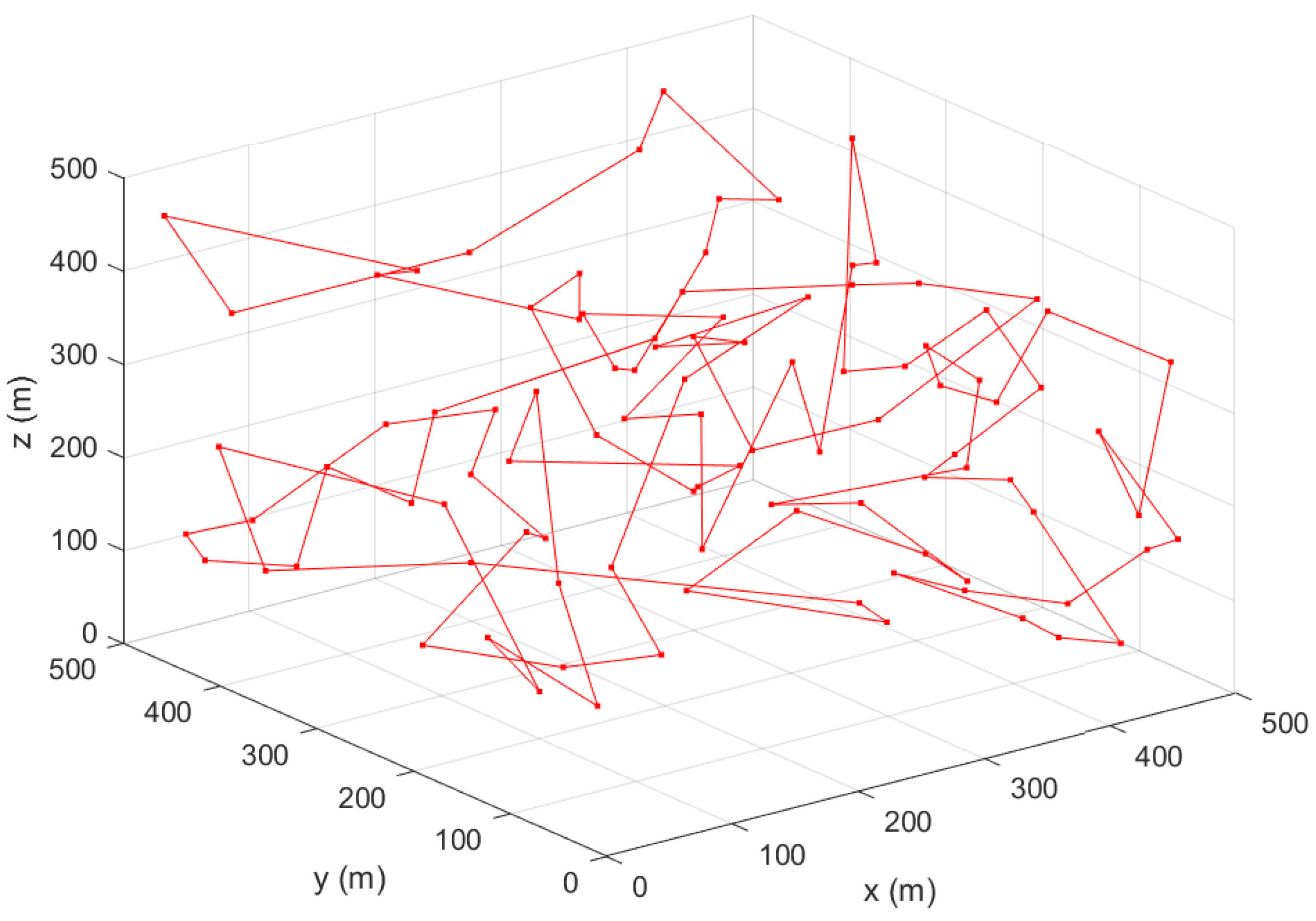
6.2. A 100-Node Scenario

This subsection considers the numerical evaluation of the proposed algorithms for a scenario with a single AGV and 100 nodes. Figure 7 illustrates 100 nodes located in a 500 m × 500 m × 500 m space.

In Figure 7, we generate the locations of 100 nodes by considering uniform random distribution for them. The locations of the 100 nodes are given as {(409, 83, 324), (454, 399, 191), (65, 157, 407), (458, 266, 268), (318, 84, 177), (50, 302, 471), (141, 133, 439), (275, 329, 277), (480, 346, 313), (484, 376, 295), (80, 227, 105), (487, 43, 152), (480, 116, 237), (244, 458, 117), (402, 78, 424), (72, 414, 99), (212, 271, 114), (459, 500, 87), (398, 41, 115), (481, 223, 219), (329, 55, 157), (19, 482, 463), (426, 4, 217), (468, 389, 94), (341, 410, 454), (380, 436, 491), (373, 44, 221), (198, 201, 57), (329, 131, 131), (87, 402, 206), (355, 217, 299), (17, 457, 133), (140, 92, 303), (25, 133, 357), (50, 74, 112), (413, 70, 60), (349, 436, 150), (160, 291, 161), (477, 276, 214), (19, 74, 255), (221, 428, 44), (192, 313, 133), (384, 177, 402), (399, 258, 16), (95, 202, 466), (246, 39, 367), (224, 121, 246), (325, 63, 292), (356, 93, 120), (379, 121, 231), (140, 210, 483), (341, 26, 277), (329, 453, 262), (83, 474, 118), (61, 247, 246), (251, 246, 314), (481 170, 341), (172, 452, 199), (294, 186, 185), (113, 57, 495), (377, 392, 20), (129, 196, 444), (254, 122, 458), (351, 203, 400), (447, 50, 51), (481, 67, 132), (275, 473, 169), (71, 480, 341), (76, 289, 70), (130, 31, 362), (422, 119, 55), (129, 178, 328), (409, 412, 249), (123, 9, 391), (466, 23, 359), (176, 86, 453), (100, 326, 447), (127, 367, 169), (310, 325, 351), (238, 227, 100), (177, 275, 17), (417, 150, 374), (294, 374, 252), (276, 96, 241), (460, 345, 454), (144, 93, 306), (380, 186, 310), (378, 314, 431), (192, 392, 404), (285, 42, 290), (39, 466, 93), (28, 389, 121), (267, 245, 445), (391, 219, 16), (469, 225, 246), (66, 155, 85), (286, 256, 491), (236, 257, 358), (7, 410, 252), (170, 399, 237)}.

By considering different subsets of these parameters, we compare the performances of the NN-, GWO-, and GA-based approaches.

6.2.1. NN-Based Approach

This subsection evaluates the performance of an NN-based solution. Figure 8 shows the NN’s achieved path planning solution in 1000 iterations in the scenario in Figure 7.

In Figure 8, the NN-based approach achieves a path length of 9045 m (please note that as an approximation algorithm, it is not an iterative algorithm).

6.2.2. GA-Based Approach

This subsection evaluates performance of a GA-based solution. Figure 9 demonstrates the GA’s achieved path planning solution in 1000 iterations in the scenario in Figure 7.

In Figure 9, the GA-based approach achieves a path length of 10,803 m in 1000 iterations as a metaheuristic which approaches the solution iteratively.

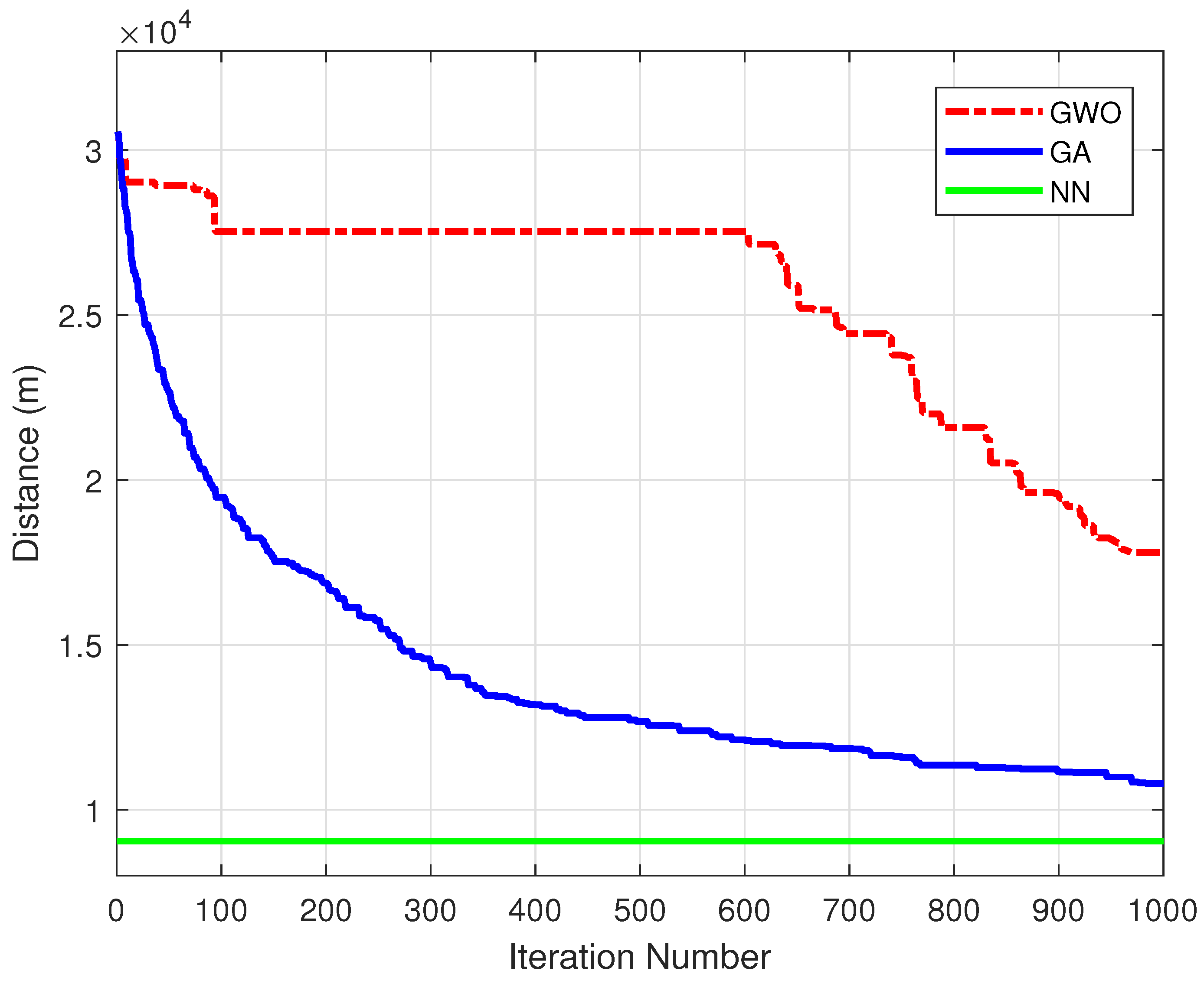
6.2.3. GWO-Based Approach

This subsection evaluates performance of a GWO-based solution. Figure 9 demonstrates the GWO’s achieved path planning solution in 1000 iterations in the scenario in Figure 7.

In Figure 10, the GWO-based approach achieves a path length of 17,794 m in 1000 iterations as a metaheuristic which approaches the solution iteratively.

6.2.4. Comparison and Discussion

Considering the general trend, the NN-based approach shows better performance than the GA-based and GWO-based approaches.

Figure 11 shows the total distance travelled by the OSA with different algorithms (NN-based approach, GWO-based approach, and GA-based approach) to visit the 100 sensor nodes given in Figure 7.

From Figure 11, we can make the following observations for the performance of the algorithms for 100-sensor scenarios. Considering the general trend, the NN-based approach performs better than the GWO-based and GA-based approaches. The NN-based approach not only gives better results than the GWO-based approach and the GA-based approach but also the NN-based approach solves in a much shorter time (0.168395 s) than the GA-based approach’s time to reach the solution (6.294668 s). The NN-based approach performs 37.4 times faster than GA-based approach. Considering all these results, increasing the number of sensor nodes from 50 nodes to 100 nodes leads to a significant difference between the NN-based approach and GA-based approach.

From

Table 2. Total path length (in terms of meters) to visit 100 nodes with NN-, GWO-, and GA-based approaches with respect to iteration number.

Iter.	100	200	300	400	500	600	700	800	900	1000
GWO	27,525	27,525	27,525	27,525	27,525	27,525	24,432	21,589	19,529	17,794
GA	19,471	16,861	14,455	13,182	12,676	12,120	11,848	11,351	11,159	10,803
NN	9045	9045	9045	9045	9045	9045	9045	9045	9045	9045

, we can make the following observations. In the first iteration, the GA-based approach and GWO-based approach started with high values of path lengths (28,000–30,000 m), while the NN-based approach achieved an efficient solution very quickly, at around 9.05 km. At the 100th iteration, the GA-based approach achieves significantly better results than GWO-based approach (8,054 m, i.e., 29% less than the GWO-based approach). At the 300th iteration, the NN-based approach achieves better results than the GWO- and GA-based approaches. At the 600th iteration, the GA-based approach achieves better results than NN-based approach. At 1000 iterations, the GA-based approach significantly outperforms the GWO-based approach (6991 m, i.e., 39.3% less than the GWO-based approach), while the NN-based approach is much faster in obtaining a shorter path than the GWO- and GA-based approaches, suggesting a practical and robust solution.

6.3. Obstacle Avoidance in 50-Node Scenario and 100-Node Scenario

This subsection evaluates performance of Obstacle-Avoided Nearest Neighbour (OANN)-based solution for the 3D TSP problem under the limitation where visiting node i just after node $i-1$ has an extreme distance cost, so it is impossible to visit.

6.3.1. Obstacle-Avoided Nearest Neighbour (OANN)-Based Approach

This subsubsection observes an Obstacle-Avoided Nearest Neighbour (OANN)-based solution for the 3D TSP problem. Figure 12 exhibits the OANN’s achieved path planning solution for visiting 50 nodes in Figure 2.

In Figure 12, the OANN-based approach achieves a path length of 6492 m (please note that as an approximation algorithm, it is not an iterative algorithm).

Figure 13 exhibits the OANN’s achieved path planning solution for visiting 100 nodes in Figure 7.

In Figure 13, the OANN-based approach achieves a path length of 9055 m.

6.3.2. Comparison and Discussion

Considering the general trend, the NN-based approach shows better performance than the OANN-based approach.

Table 3. Total distance (in terms of meters) with NN-based approach and OANN-based approach under 50-node and 100-node scenarios.

Iteration	Achieved Length
NN with 50 nodes	6358
OANN with 50 nodes	6492
NN with 100 nodes	9045
OANN with 100 nodes	9055

shows the total travelled distance by the AUV with the NN-based approach and OANN-based approach under the 50-node scenario in Figure 2 and the 100-node scenario in Figure 7.

From Table 3, we can make the following observations. Under the 50-node scenario, the NN-based approach and OANN-based approach achieve almost the same performance with just a slight difference. (the difference between their achieved path lengths is 138 m, that is, 2.13% less than the OANN-based approach). Similarly, under the 100-node scenario, the NN-based approach and OANN-based approach achieve almost the same performance with just a slight difference (the difference between their achieved path lengths is 10 m, that is, 0.11% less than the OANN-based approach). We expect the difference in the 100-node scenario to be much less than the difference in the 50-node scenario because increasing the number of nodes increases the alternative destination for a node much more. In this case, the probability of preferring a node with the next ID can decrease considerably.

7. Conclusions

Because environmental monitoring is becoming more and more important, research is currently focused on longer ranges and broader exploratory ranges. Here, we present an efficient path planning technique that charges the wireless sensor network (WSN) using an autonomous ground vehicle with a limited battery pack, and we theoretically analyse the total energy consumption of the network. We tackle the problem from the perspective of charging because the WSN has a finite amount of energy. Using a large number of AGVs is an efficient method of charging the WSN to extend the exploration network. Furthermore, the exploration range and charging efficiency can be significantly increased by selecting suitable diving locations and designing a path that takes the node’s location and data flow into consideration.

Automated ground vehicles (AGVs) can have their data collection problems resolved using the Nearest Neighbour-based approach, the Grey Wolf Optimizer-based approach, and the Genetic Algorithm-based approach. Simulations demonstrate that the AGV route planning system finds a better solution and converges more quickly than previous algorithms by utilising a Nearest Neighbour-based technique.

The Obstacle-Avoided Nearest Neighbour (OANN)-based solution for the 3D TSP problem is under a physical limitation or obstacle where visiting node i just after node $i-1$ has an extreme distance cost, so it is impossible to visit. Even in this case, Obstacle-Avoided Nearest Neighbour (OANN)-based approach achieves almost the same performance (just a 2.13% longer path for the 50-node scenario and 0.11% longer path for the 100-node scenario) as the performance of Nearest Neighbour (OANN)-based approach in a no-limitation case.

In the future, we can tackle the energy-aware path planning problem by considering different models for the limitations occurring between some sensor pairs. As a future work, we may tackle the energy-aware path planning problem by considering imperfect accuracy to hit the sensor nodes.

References

1. Felemban, E.; Shaikh, F.K. Underwater sensor network applications: A comprehensive survey. Int. J. Distrib. Sens. Netw. 2015, 11, 896832–896845. [Google Scholar] [CrossRef]
2. Raghunathan, V.; Schurgers, C.; Park, S.; Srivastava, M.B. Energy-aware wireless microsensor networks. IEEE Signal Process. Mag. 2002, 19, 40–50. [Google Scholar] [CrossRef]
3. Alcaina, J.; Cuenca, Á.; Salt, J.; Zheng, M.; Tomizuka, M. Energy-Efficient Control for an Unmanned Ground Vehicle in a Wireless Sensor Network. J. Sens. 2019, 2019, 7085915. [Google Scholar] [CrossRef]
4. Eris, C.; Gul, O.M.; Boluk, P.S. An Energy-Harvesting Aware Cluster Head Selection Policy in Underwater Acoustic Sensor Networks. In Proceedings of the 2023 International Balkan Conference on Communications and Networking, İstanbul, Turkiye, 5–8 June 2023; pp. 1–5. [Google Scholar]
5. Eris, C.; Gul, O.M.; Boluk, P.S. A Novel Medium Access Policy based on Reinforcement Learning in Energy-Harvesting Underwater Sensor Networks. Sensors 2024, 24, 1–21. [Google Scholar]
6. Eris, C.; Gul, O.M.; Boluk, P.S. A novel reinforcement learning based routing algorithm for energy management in networks. J. Ind. Manag. Optim. 2024, 20, 3678–3696. [Google Scholar] [CrossRef]
7. Li, Q.; Du, X. Energy-efficient data compression for underwater wireless sensor networks. IEEE Access 2020, 8, 73395–73406. [Google Scholar]
8. Cheng, F.; Wang, J. Energy-efficient routing protocols in underwater wireless sensor networks: A survey. IEEE Commun. Surv. Tutor. 2014, 16, 277–294. [Google Scholar]
9. Khan, A.U.; Somasundaraswaran, K. Wireless charging technologies for underwater sensor networks: A comprehensive review. IEEE Commun. Surv. Tutor. 2018, 20, 674–709. [Google Scholar]
10. Pendergast, D.R.; DeMauro, E.P. A rechargeable lithium-ion battery module for underwater use. J. Power Sources 2011, 196, 793–800. [Google Scholar] [CrossRef]
11. Blidberg, D.R. The development of autonomous underwater vehicles (AGV); a brief summary. In Proceedings of the IEEE ICRA, Seoul, Republic of Korea, 21–26 May 2001; Volume 4, pp. 122–129. [Google Scholar]
12. Ghafoor, H.; Noh, Y. An overview of next-generation underwater target detection and tracking: An integrated underwater architecture. IEEE Access 2019, 7, 98841–98853. [Google Scholar] [CrossRef]
13. Xie, L.; Shi, Y. Rechargeable sensor networks with magnetic resonant coupling. Recharg. Sens. Netw. Technol. Theory Appl. Introd. Energy Harvest. Sens. Netw. 2014, 9, 31–68. [Google Scholar]
14. Lee, J.; Yun, N. A focus on comparative analysis: Key findings of MAC protocols for underwater acoustic communication according to network topology. In Proceedings of the Multimedia, Computer Graphics and Broadcasting: International Conference, Jeju Island, Republic of Korea, 8–10 December 2011. [Google Scholar]
15. Zenia, N.Z.; Aseeri, M. Energy-efficiency and reliability in MAC and routing protocols for underwater wireless sensor network: A survey. J. Netw. Comput. Appl. 2016, 71, 72–85. [Google Scholar] [CrossRef]
16. Khan, M.T.R.; Ahmed, S.H. An energy-efficient data collection protocol with AGV path planning in the internet of underwater things. J. Netw. Comput. Appl. 2019, 135, 20–31. [Google Scholar] [CrossRef]
17. Su, Y.; Xu, Y. HCAR: A Hybrid-Coding-Aware Routing Protocol for Underwater Acoustic Sensor Networks. IEEE Internet Things J. 2023, 10, 10790–10801. [Google Scholar] [CrossRef]
18. Kumar, V.; Sandeep, D. Multi-hop communication based optimal clustering in hexagon and voronoi cell structured WSNs. AEU-Int. J. Electron. Commun. 2018, 93, 305–316. [Google Scholar] [CrossRef]
19. Xie, R.; Jia, X. Transmission-efficient clustering method for wireless sensor networks using compressive sensing. IEEE Trans. Parallel Distrib. Syst. 2013, 25, 806–815. [Google Scholar]
20. Yadav, S.; Kumar, V. Hybrid compressive sensing enabled energy efficient transmission of multi-hop clustered UWSNs. AEU-Int. J. Electron. Commun. 2019, 110, 152836–152851. [Google Scholar] [CrossRef]
21. Sun, Y.; Zheng, M.; Han, X.; Li, S.; Yin, J. Adaptive clustering routing protocol for underwater sensor networks. Ad Hoc Netw. 2022, 136, 102953–102965. [Google Scholar] [CrossRef]
22. Fan, R.; Jin, Z. A time-varying acoustic channel-aware topology control mechanism for cooperative underwater sonar detection network. Ad Hoc Netw. 2023, 149, 103228. [Google Scholar] [CrossRef]
23. Liu, C.F.; Zhao, Z. A distributed node deployment algorithm for underwater wireless sensor networks based on virtual forces. J. Syst. Archit. 2019, 97, 9–19. [Google Scholar] [CrossRef]
24. Wei, L.; Han, J. Topology Control Algorithm of Underwater Sensor Network Based on Potential-Game and Optimal Rigid Sub-Graph. IEEE Access 2020, 8, 177481–177494. [Google Scholar] [CrossRef]
25. Zhu, R.; Boukerche, A. A trust management-based secure routing protocol with AGV-aided path repairing for Underwater Acoustic Sensor Networks. Ad Hoc Netw. 2023, 149, 103212–103225. [Google Scholar] [CrossRef]
26. Yan, Z.; Li, Y. Data collection optimization of ocean observation network based on AGV path planning and communication. Ocean Eng. 2023, 282, 114912–114927. [Google Scholar] [CrossRef]
27. Shen, G.; Zhu, X. Research on phase combination and signal timing based on improved K-medoids algorithm for intersection signal control. Wirel. Commun. Mob. Comput. 2020, 2020, 3240675. [Google Scholar] [CrossRef]
28. Yan, J.; Yang, X. Energy-efficient data collection over AUV-assisted underwater acoustic sensor network. IEEE Syst. J. 2018, 12, 3519–3530. [Google Scholar] [CrossRef]
29. Kan, T.; Mai, R. Design and analysis of a Three-Phase wireless charging system for lightweight autonomous underwater vehicles. IEEE Trans. Power Electron. 2018, 33, 6622–6632. [Google Scholar] [CrossRef]
30. Ramos, A.G.; García-Garrido, V.J. Lagrangian coherent structure assisted path planning for transoceanic autonomous underwater vehicle missions. Sci. Rep. 2018, 8, 4575. [Google Scholar] [CrossRef]
31. Cheng, C.; Sha, Q. Path planning and obstacle avoidance for AGV: A review. Ocean Eng. 2021, 235, 109355–109368. [Google Scholar] [CrossRef]
32. Kumar, S.V.; Jayaparvathy, R. Efficient path planning of AGVs for container ship oil spill detection in coastal areas. Ocean Eng. 2020, 217, 107932–107945. [Google Scholar] [CrossRef]
33. Golen, E.; Mishra, F. An underwater sensor allocation scheme for a range dependent environment. Comput. Netw. 2010, 54, 404–415. [Google Scholar] [CrossRef]
34. Yi, Y.; Yang, G.S. Energy balancing and path plan strategy for rechargeable underwater sensor network. In Proceedings of the 2022-4th International Conference on Advances in Computer Technology, Suzhou, China, 22–24 April 2022. [Google Scholar]
35. Cui, Y.; Zhu, P.; Lei, G.; Chen, P.; Yang, G. Energy-Efficient Multiple Autonomous Underwater Vehicle Path Planning Scheme in Underwater Sensor Networks. Electronics 2023, 12, 3321. [Google Scholar] [CrossRef]
36. Zhang, H.; Zhang, Y.; Liu, C.; Zhang, Z. Energy efficient path planning for autonomous ground vehicles with ackermann steering. Robot. Auton. Syst. 2023, 162, 104366. [Google Scholar] [CrossRef]
37. Gul, O.M.; Acarer, T. Robust and Energy-Aware Path Planning by Autonomous Underwater Vehicle in Underwater Wireless Sensor Networks for Monitoring Maritime Transportation. EMO Sci. J. 2024, 14, 71–85. [Google Scholar]
38. Gul, O.M. A Novel Energy-Aware Path Planning by Autonomous Underwater Vehicle in Underwater Wireless Sensor Networks. Turk. J. Marit. Mar. Sci. 2024, 10, 1–14. [Google Scholar]
39. Pop, P.C.; Cosma, O.; Sabo, C.; Sitar, C.P. A comprehensive survey on the generalized traveling salesman problem. Eur. J. Oper. Res. 2024, 314, 819–835. [Google Scholar] [CrossRef]
40. Davendra, D. Travelling Salesman Problem, Theory and Applications; InTech: Houston TX, USA, 2010. [Google Scholar]
41. Johnson, D.S.; McGeoch, L.A. The Traveling Salesman Problem: A Case Study, Local Search in Combinatorial Optimization; John Wiley & Sons: Hoboken, NJ, USA, 1997; pp. 215–310. [Google Scholar]
42. Gutin, G.; Punnen, A. (Eds.) The Traveling Salesman Problem and Its Variations; Combinatorial Optimization; Kluwer: Dordrecht, The Netherlands, 2002; Volume 12. [Google Scholar]
43. Hoffman, K.L.; Padberg, M. Traveling salesman problem. In Encyclopedia of Operations Research and Management Science; Gass, S.I., Harris, C.M., Eds.; Springer: New York, NY, USA, 2001. [Google Scholar]
44. Gutin, G.; Yeo, A.; Zverovitch, A. Exponential Neighborhoods and Domination Analysis for the TSP. In The Traveling Salesman Problem and Its Variations; Gutin, G., Punnen, A.P., Eds.; Springer: Berlin/Heidelberg, Germany, 2007. [Google Scholar]
45. Mirjalili, S.; Mirjalili, S.M.; Lewis, A. grey wolf optimizer. Adv. Eng. Softw. 2014, 69, 46–61. [Google Scholar] [CrossRef]
46. Goldberg, D.E. Genetic Algorithms in Search, Optimization and Machine Learning; Addison-Wesley Longman Publishing Co., Inc.: Upper Saddle River, NJ, USA, 1989. [Google Scholar]
47. Bonabeau, E.; Dorigo, M.; Theraulaz, G. Swarm Intelligence: From Natural to Artificial Systems (No. 1); Oxford University Press: Oxford, UK, 1999. [Google Scholar]
Figure 1. In this wireless sensor network (WSN), an automated guided vehicle (AGV) is utilized to collect data from all fifteen sensors (S1, S2,…, S15) that are monitoring the environment with the purpose of identifying anomalies and dangers in order to decrease the likelihood of accidents occurring. Following the completion of the compilation of all of the data, they should be transmitted to the data sink, which is the entity that is accountable for collecting all of the data and evaluating them.
Wevj 15 00383 g001
Figure 2. Locations of sensors.
Wevj 15 00383 g002
Figure 3. Achieved path planning solution by Nearest Neighbour.
Wevj 15 00383 g003
Figure 4. Achieved path planning solution with GA in 1000 iterations.
Wevj 15 00383 g004
Figure 5. Achieved path planning solution with GWO in 1000 iterations.
Wevj 15 00383 g005
Figure 6. Achieved path lengths for visiting 100 nodes with NN-based approach, GWO-based approach, and GA-based approach in 1000 iterations.
Wevj 15 00383 g006
Figure 7. The coordinates of the 100 sensor nodes.
Wevj 15 00383 g007
Figure 8. Achieved path planning solution with NN-based approach.
Wevj 15 00383 g008
Figure 9. The achieved (10,803 m) path planning solution for visiting the 100 nodes with the GA in 1000 iterations.
Wevj 15 00383 g009
Figure 10. The achieved (17,794 m) path planning solution for visiting the 100 nodes with the GWO in 1000 iterations.
Wevj 15 00383 g010
Figure 11. The achieved path lengths for visiting the 100 nodes by all the algorithms (NN-based approach, GWO-based approach, and GA-based approach) in 1000 iterations.
Wevj 15 00383 g011
Figure 12. Achieved path planning solution for visiting the 50 nodes by AUV with OANN under limitations.
Wevj 15 00383 g012
Figure 13. Achieved path planning solution for visiting the 100 nodes by AUV with OANN under limitations.
Wevj 15 00383 g013