Abstract
To improve the tracking accuracy and robustness of the path-tracking control model for intelligent vehicles under longitudinal and lateral coupling constraints, this paper utilizes the Kalman filter algorithm to design a longitudinal and lateral coordinated control (LLCC) strategy optimized by adaptive sliding mode control (ASMC). First, a three-degree-of-freedom (3-DOF) vehicle dynamics model was established. Next, under the fuzzy adaptive Unscented Kalman filter (UKF) theory, the vehicle state parameter estimation and road adhesion coefficient (RAC) observer were designed to estimate vehicle speed (VS), yaw rate (YR), sideslip angle (SA), and RAC. Then, a layered control concept was adopted to design the path-tracking controller, with a target VS, YR, and SA as control objectives. An upper-level adaptive sliding mode controller was designed using RBF neural networks, while a lower-level tire force distribution controller was designed using distributed sequential quadratic programming (DSQP) to obtain an optimal tire driving force. Finally, the control strategy was validated using Carsim and Matlab/Simulink software under different road adhesion coefficients and speeds. The findings indicate that the optimized control strategy is capable of adaptively adjusting control parameters to accommodate various complex conditions, enhancing the tracking precision and robustness of vehicles even further.
1. Introduction
As intelligent transportation technology advances, there is growing focus on the driving safety of intelligent vehicles. To tackle the problems of reduced path-tracking precision and reduced robustness in vehicle stability control for intelligent vehicles, longitudinal and lateral coordinated control technology has gradually become a research hotspot. This technology enhances the tracking precision and stability of vehicles in complex environments by coordinating longitudinal and lateral control systems. Under complex conditions like a high VS and a low RAC, traditional control methods include proportional integral derivative control [1,2], linear quadratic regulators [3,4], SMC [5,6], and model predictive control [7,8]. Traditional control methods perform well in certain scenarios, but they often exhibit limitations in adaptability and robustness when confronted with varying environmental conditions. For instance, while PID control is simple to implement, it tends to result in overshoot and steady-state errors when dealing with nonlinear and highly dynamic scenarios. Although LQR and MPC improve path-tracking accuracy, their computational complexity becomes a constraint in scenarios with high real-time performance requirements. These methods often face challenges in terms of robustness and adaptability to dynamic road conditions. However, advanced coordinated control technologies combining vehicle dynamics models with advanced control algorithms have emerged as promising solutions. Techniques such as fuzzy logic control [9,10], adaptive control [11,12], and robust control [13,14] have been developed to address the limitations of the traditional methods. However, these approaches still have certain limitations. For instance, the design of rule sets in fuzzy control relies heavily on expert experience, and while adaptive control enhances the system’s responsiveness, it may still suffer from reduced control accuracy when dealing with external disturbances.
In recent years, machine learning and neural networks have been integrated into control strategies to further enhance the adaptability and robustness of vehicle control systems. For instance, Yang designed an MPC and fuzzy PID method to achieve coordinated optimization of longitudinal and lateral control, but the combination of algorithms in-creased the system complexity [15]. This study improves control accuracy and stability while reducing system complexity. Li designed a driving controller under LQR, but it was challenging to balance the control weights between the autonomous driving system and the driver’s intentions in practical driving scenarios [16]. These data-driven approaches are increasingly being used to optimize control performance, especially in scenarios involving high-speed and low-adhesion conditions. Other researchers have explored hybrid control strategies, combining traditional control algorithms with advanced techniques. Chu proposed a method using priority weights, combining the LQR path-tracking method with a fuzzy controller, but the dynamic adjustment of priority weights still needs to be considered in practical applications [17]. However, the DSQP algorithm proposed in this study further optimizes tire force distribution, enabling better vehicle stability in complex environments. Lhoussain designed a sliding mode controller that considers disturbance and uncertainty factors, but the controller relies heavily on model parameters and upper bounds of disturbances [18]. These hybrid approaches aim to strike a balance between control accuracy and system complexity. Yang designed a MPC strategy for longitudinal control, achieving precise control of vehicle dynamic behavior through multi-objective optimization. However, the convergence speed of multi-objective optimization algorithms can become a limitation when addressing complex and dynamically changing road environments [19]. Moreover, strategies incorporating predictive control methods have shown promise in handling dynamically changing environments. Zhou designed a bidirectional memory autoencoder to identify driving models, combined with a fuzzy controller, but the practical experiment requires substantial data support [20]. This study reduces dependency on model parameters by incorporating RBF neural networks, while also enhancing robustness against disturbances. Zhang proposed a control strategy using quintic polynomials as reference paths, combined with a multi-objective optimization model predictive control, but the complexity of path planning and dynamic environmental changes in real road conditions may lead to deviations between the planned and the actual paths [21]. Lai designed LLCC strategies for curved road conditions, proposing a comprehensive control strategy combining automatic emergency braking and lane-keeping assist systems, but in complex road environments the control system’s response may be delayed [22]. Qin proposed a multi-vehicle coordinated control scheme, optimizing inter-vehicle coordination using a hierarchical nonlinear model predictive control algorithm, but it requires processing a large amount of coordination control data, leading to high computational complexity [23].
These studies provide various strategies that effectively address path deviation and sideslip issues encountered in intelligent-vehicle path tracking and vehicle stability control during sharp turns [24]. However, to further enhance the control performance of intelligent vehicles under a high VS and a low RAS, including wet, slippery, or icy conditions, longitudinal and lateral coordinated control technology [25] has become the current challenge. Wang studied a trajectory-tracking control algorithm for electric vehicles under terminal SMC, RBF neural networks, and fuzzy logic algorithms, improving the accuracy of lateral control while reducing control system chattering [26]. Wang designed a multi-input-output three-step nonlinear control method for LLCC, rigorously proving the stability of the closed-loop system under the Lyapunov function. However, this method typically only finds local optimal solutions for non-convex optimization problems, potentially leading to chattering issues [27]. Feng proposed a model-free ASMC method by combining model-free adaptive control with SMC, which better enhances control effectiveness and disturbance rejection performance [28]. Guo designed a state feedback lateral control system, effectively handling uncertainties and external disturbances to generate the desired front wheel steering angle and external yaw moment, thereby enhancing the control system’s robustness to model uncertainties and external disturbances, improving vehicle stability and control accuracy [29].
Our research shares common goals with the aforementioned work, specifically in improving vehicle path-tracking accuracy and stability under complex road conditions, while minimizing system resource consumption. We also employ intelligent control algorithms, such as adaptive control and fuzzy control, to address the challenges of controlling vehicles in dynamic environments. While there are similarities with other studies, we have made several key improvements. By combining RBF neural networks with adaptive sliding mode control (ASMC), our control system not only enhances path-tracking accuracy but also significantly improves robustness against external disturbances. Additionally, the introduction of the DSQP algorithm for optimizing tire force distribution has led to a marked improvement in vehicle stability under complex road conditions.
Building on the foundation of the above studies, this article designs a LLCC-ASMC strategy to improve intelligent vehicle path tracking. This strategy designs a fuzzy adaptive unscented Kalman filter observer and an ASMC under RBF neural network. The integration of a fuzzy adaptive unscented Kalman filter enhances vehicle state and road adhesion estimation. The combination of RBF neural networks with sliding mode control improves system robustness and adaptability. The DSQP algorithm optimizes tire force distribution, significantly enhancing both path-tracking performance and vehicle stability under various conditions. The main content and objectives of this study are as follows:
- (1)
- Under the 3-DOF vehicle dynamics model, a fuzzy adaptive unscented Kalman filter observer is designed to estimate the VS, YR, SA, and RAC.
- (2)
- To address instability and external disturbance issues in vehicle tracking control, an ASMC under RBF neural networks is designed to calculate the total longitudinal force, the total lateral force, and the total yaw moment required by the vehicle.
- (3)
- The optimal tire driving force is obtained using a DSQP algorithm, significantly enhancing the path-tracking performance.
- (4)
- The state estimation algorithm and the path-tracking algorithm are validated using Carsim and Matlab/Simulink under different RACs and VSs, improving the vehicle’s tracking accuracy, stability, and robustness.
2. Vehicle Dynamics Modeling
2.1. Vehicle Dynamics Model
The vehicle dynamics model is an essential tool for describing and analyzing vehicle motion behavior. The 3-DOF vehicle dynamics model considers three primary motion freedoms of vehicles: longitudinal, lateral, and yaw around the center of mass. As shown in Figure 1, this model provides a comprehensive understanding of vehicle dynamic behavior and offers a solid theoretical foundation for designing and optimizing path-tracking control algorithms.
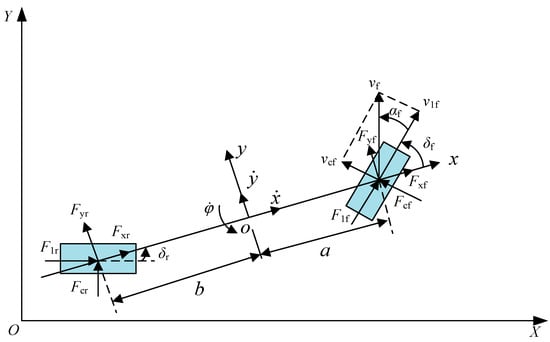
Figure 1.
Vehicle Dynamics Model.
The longitudinal dynamics equation describes the force balance in longitudinal direction, primarily considering driving force, air, rolling, and gradient resistance. The equation is formulated as follows:
where is the vehicle mass, is the vehicle’s longitudinal acceleration, is the total longitudinal driving force, is the air resistance, is the rolling resistance, and is the gradient resistance. These forces collectively determine the vehicle’s longitudinal acceleration . The driving force propels the vehicle forward, while the resistive forces , , and counteract this motion. The expressions for each force are as follows:
where is the air density, is the air resistance coefficient, is the vehicle’s frontal area, is the vehicle speed, is the rolling resistance coefficient, is the gravitational acceleration, and is the gradient angle.
The lateral dynamics equation describes the force balance in the lateral direction of the vehicle, mainly considering lateral tire forces. The lateral dynamics are critical in determining how the vehicle handles during maneuvers such as turning. The lateral force is affected by factors such as the tire grip, the vehicle speed, and the cornering radius. The equation is as follows:
where is the vehicle’s lateral acceleration and is the total lateral force.
The yaw dynamics equation describes the rotational motion around the vehicle, primarily influenced by the lateral forces of the front and rear tires and the vehicle’s inertial characteristics. The equation is as follows:
where is the yaw moment of inertia, is the yaw acceleration, and represent the distance from the center of mass to the front and rear axles, and and represent the lateral force of the front and rear tires.
The yaw dynamics play a crucial role in vehicle handling, particularly during steering maneuvers. The yaw moment of inertia and the forces at the front and rear wheels determine how quickly and accurately the vehicle can change its direction. This equation is fundamental for understanding vehicle stability and control during turning and lane-changing maneuvers.
2.2. Tire Model and Inverse Model under Dugoff Model
Slip ratio is an indicator describing the degree of slip of the tire relative to the ground. It is usually divided into longitudinal slip ratio and lateral slip ratio.
where is the vehicle speed, is the tire radius, is the tire’s angular velocity, is the lateral speed, and is the longitudinal speed.
The Dugoff model represents longitudinal and lateral forces as functions of the slip ratio, and it assumes that the tire’s friction force is jointly affected by the longitudinal and the lateral slip ratio. The Dugoff model provides a non-linear relationship between the slip ratio and the tire forces. This is critical for accurately modeling tire behavior under different driving conditions, such as cornering at high speeds or during emergency braking.
where is the longitudinal stiffness coefficient, is the road friction coefficient, is the vertical load, is the lateral stiffness coefficient, and is the slip angle.
The inverse model is used to calculate the slip ratio and slip angle for a given longitudinal and lateral force. The inverse solutions for and are as follows:
Through the inverse model calculation, the slip ratio and slip angle under given longitudinal and lateral forces can be obtained, further calculating the front wheel angle, significantly improving the vehicle’s control accuracy and stability.
3. State Observers under the KF Algorithm
3.1. Vehicle State Estimation
3.1.1. Establishment of Vehicle State Estimation System
In the vehicle dynamics model, considering complex dynamic behavior and control requirements of the vehicle, a nonlinear 3-DOF model for longitudinal, lateral, and yaw motion was established. The model includes the following equations:
where and are the longitudinal and lateral forces of each wheel, and is the rolling resistance coefficient.
To simplify control design and computation, the above nonlinear model is transformed into a state-space form. The process noise captures uncertainties in the system, such as modeling errors or environmental disturbances. Accurate state estimation is critical for vehicle control, as it provides real-time feedback on the vehicle’s behavior. This equation forms the basis for applying estimation techniques like the Kalman filter to improve control accuracy. The state-space equations can be represented as follows:
where is the system dynamic equation, is the measurement equation, and and are the process noise and the measurement noise, respectively. The specific forms are:
The state-space model can be used with the UKF algorithm for the estimation of vehicle states, providing reliable data support for vehicle path-tracking control strategies.
3.1.2. Adaptive Adjustment Strategy Based on Fuzzy Control
To improve the adaptability and robustness of the UKF algorithm, a fuzzy adaptive mechanism was introduced to dynamically adjust the filtering parameters. The adaptive adjustment of the measurement noise covariance matrix R was achieved through a fuzzy logic controller, which dynamically modified the value of based on the difference between the actual covariance of the measurement variables and the theoretical covariance predicted by the Unscented Kalman filter (UKF). Specifically, the fuzzy logic controller took the error e as its input. The controller then adjusted the value of proportionally by introducing a correction factor that is determined by fuzzy inference rules. These rules are designed to increase or decrease depending on the magnitude of the error e, thereby allowing the system to adapt to changing sensor performance and measurement conditions in real time. This mechanism ensures that the UKF remains responsive and accurate even in the presence of varying measurement noise. The measurement noise covariance matrix is usually set to a fixed value. However, in practical applications, due to the influence of sensor performance, the measurement accuracy varies under different conditions, causing the measurement noise covariance matrix to change accordingly. Therefore, this article proposes an adaptive adjustment strategy under fuzzy control to improve state estimation accuracy by adjusting in real time.
The calculation formula for the actual and theoretical covariance of the measurement variables is as follows:
where is the actual measurement value, is the measurement matrix, is the predicted state vector, is the state estimation error covariance matrix, and is the measurement noise covariance matrix.
The difference between the actual covariance and the theoretical covariance is as follows:
Adaptive adjustment strategy: Set measurement noise covariance matrix at time as , and , where is the adjustment variable for the covariance matrix .
3.1.3. Simulation Analysis of Vehicle State Estimation
To verify the effectiveness of the state estimation algorithm, it was validated by Carsim 2019 and Matlab/Simulink 2022 simulation software.
- (1)
- Scenario 1: 60 km/h Double Lane Change (DLC)
In Carsim, the initial VS was prescribed at 60 km/h, with a RAC of 0.85. The simulation scenario was DLC. The SA and YR were set to 0. To realistically simulate the noise characteristics detected by sensors, random noise was added to the lateral acceleration during the simulation. The simulation results are in Figure 2.
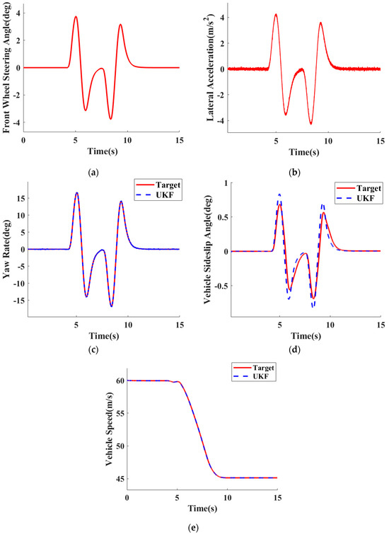
Figure 2.
60 km/h DLC: (a) Front wheel steering angle; (b) lateral acceleration; (c) YR; (d) SA and (e) longitudinal speed.
The simulation results from Figure 2a–e collectively demonstrate the performance of the proposed control system during a 60 km/h double lane change maneuver. The front wheel steering angle showed controlled and symmetrical steering inputs with peaks of ±4°, indicating the effective management of the dynamic steering demands. The lateral acceleration peaked at ±4 m/s2, further validating the system’s ability to handle the lateral forces while maintaining vehicle stability. The yaw rate closely followed the target values, with the UKF accurately estimating the vehicle’s dynamic behavior, essential for precise trajectory tracking. Similarly, the sideslip angle remained within a small range of ±0.5°, demonstrating the control system’s capability to prevent excessive lateral slip and maintain stability during the maneuver. Lastly, the longitudinal speed confirmed that the vehicle speed is accurately tracked by the UKF, showing a close match with the target speed, thus maintaining longitudinal control. Altogether, these results validate the effectiveness of the proposed control system in managing both the lateral and the longitudinal dynamics of the vehicle during high-speed lane change maneuvers.
- (2)
- Scenario 2: 100 km/h DLC
In Carsim, the initial VS was prescribed at 100 km/h, with a RAC of 0.85. The simulation scenario was DLC. The SA and YR were set to 0. The simulation results are shown in Figure 3.

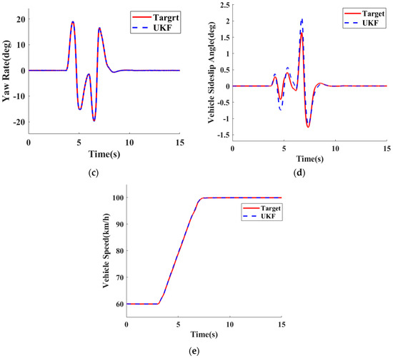
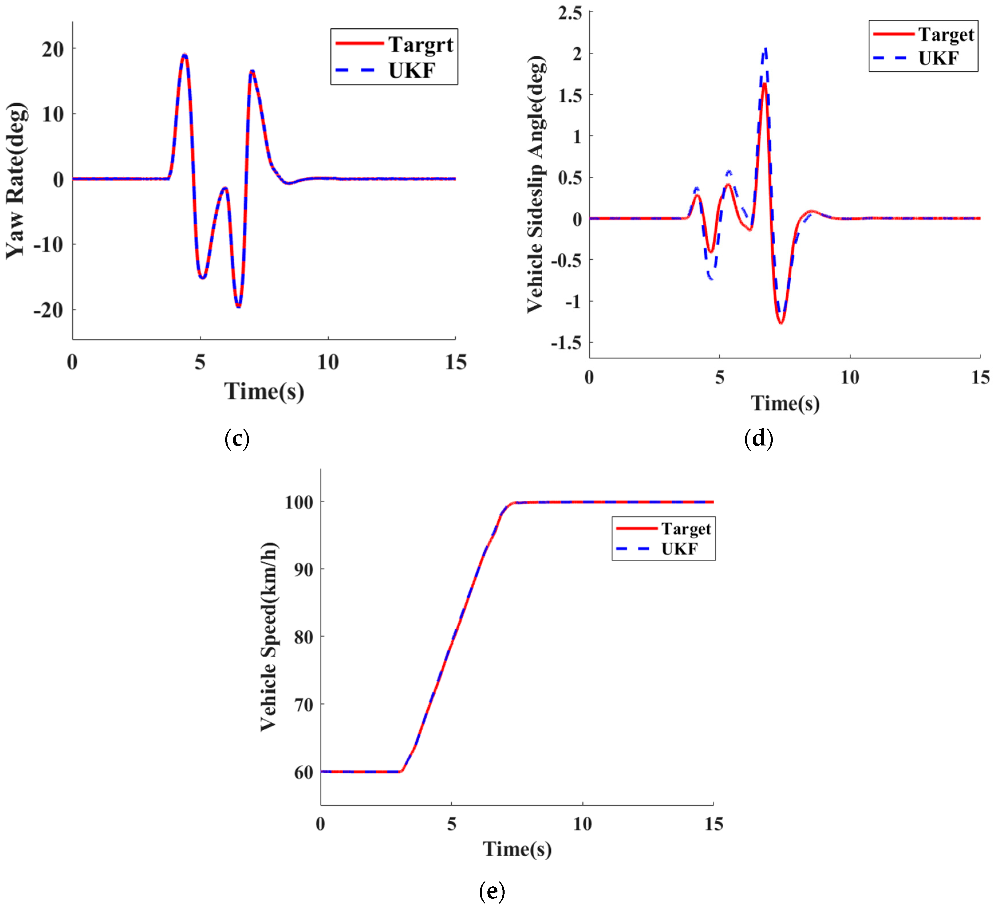
Figure 3.
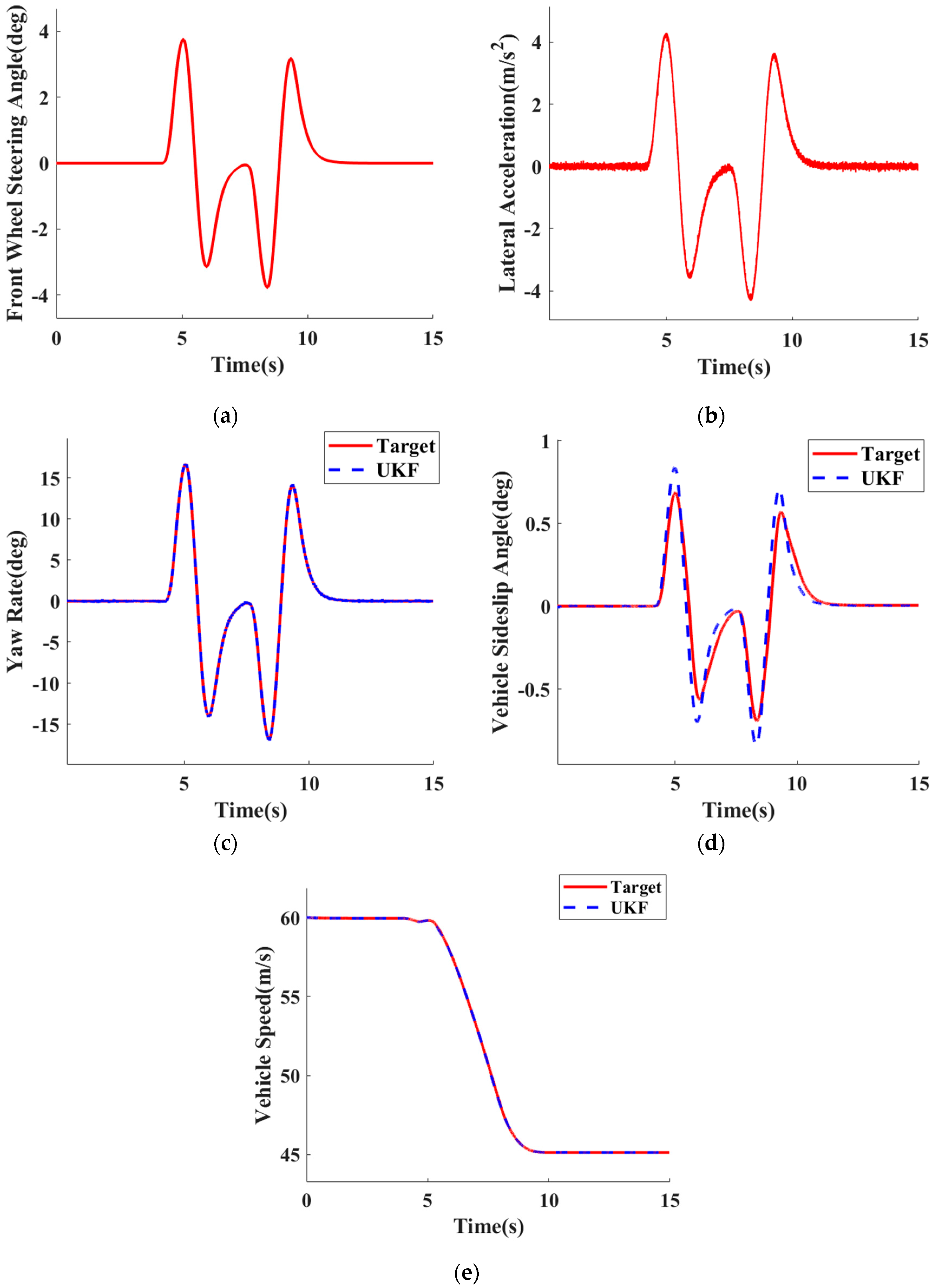
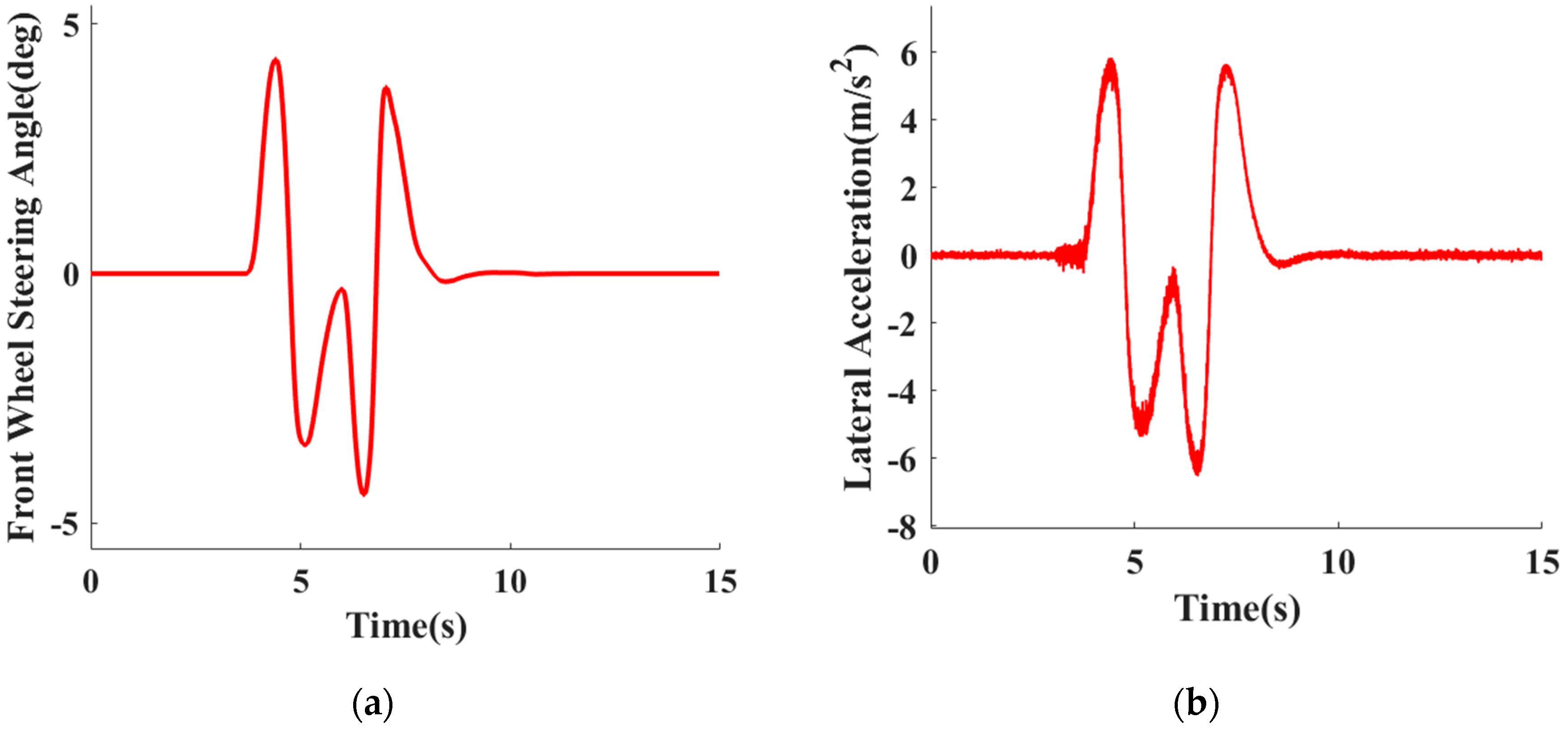
100 km/h DLC: (a) front wheel steering angle; (b) lateral acceleration; (c) YR; (d) SA and (e) longitudinal speed.
The simulation results for the 100 km/h double lane change scenario demonstrate the robust performance of the proposed control system under high-speed conditions. The front wheel steering angle reached peak values of ±5°, reflecting the increased steering input required at higher speeds, while the system quickly stabilized the vehicle after each maneuver. The lateral acceleration peaked at 6 m/s2 and −7 m/s2, indicating significant lateral forces, yet the control system effectively managed these forces, maintaining vehicle stability throughout the maneuver. The fuzzy adaptive UKF algorithm can adaptively adjust the observation noise, achieving dynamic adjustment of the covariance matrix R, effectively reducing observation errors caused by noise interference. The yaw rate, with peaks of ±20°/s, was closely tracked by the UKF, ensuring precise path following and confirming the control system’s ability to handle quick rotational dynamics at high speeds. Despite the increased speed, the sideslip angle remained within a controllable range, peaking at 1.5°, which prevents excessive lateral slip and contributes to overall vehicle stability. Additionally, the vehicle speed was accurately maintained, with the UKF providing precise speed estimations that closely matched the target values, ensuring stable longitudinal control. These results collectively validate the effectiveness of the proposed control strategy in managing both lateral and longitudinal dynamics during high-speed maneuvers, confirming its applicability in complex driving scenarios.
3.2. Road Adhesion Coefficient Estimation under UKF
3.2.1. Establishment of RAC Estimation System
The RAC is an important parameter that affects vehicle dynamic behavior. An accurate estimation of the RAC is crucial for stability control, active safety systems, and path planning for autonomous vehicles. UKF uses unscented transformation to approximate the distribution of the state of nonlinear systems. Due to its superiority in handling nonlinear systems, it has become an effective tool for estimating the road adhesion coefficient. The main steps include:
Generating a set of sigma points based on the current state mean and covariance :
Predicting state for each sigma point:
Calculating the predicted mean and covariance:
Converting the predicted state sigma points through the observation equation and calculating the predicted observation mean:
Calculating the predicted observation covariance and cross-covariance:
Calculating the Kalman gain and updating the state estimation:
Through the above UKF algorithm steps, real-time estimation of the vehicle road adhesion coefficient can be achieved. Because of its excellence in managing nonlinear systems, UKF can effectively improve estimation accuracy, providing reliable parameter support for vehicle stability control.
3.2.2. Simulation Analysis of RAC Estimation
The RAC is a crucial parameter that affects both vehicle dynamic characteristics and driving safety. In vehicle dynamic control systems, accurately estimating the RAC is essential for improving driving safety. This study conducted simulation analysis of the RAC estimation algorithm under open-road and joint-road conditions in Carsim.
- (1)
- Scenario 1: Open Road
In Carsim, the VS was maintained at 100 km/h with a sinusoidal steering input. The RACs were set at 0.8 and 0.3 for the open road. The initial values of the RAC for the four wheels were all set to 0. The simulation results are shown in Figure 4. In the initial stage, the adhesion coefficients of FL1 and RL3 rapidly rose to approximately 0.8, then stabilized around 0.8 after 0.5 s. The adhesion coefficients of FR2 and RR4 quickly approached 0.3, demonstrating the UKF algorithm’s better tracking accuracy and convergence performance for estimating road adhesion coefficients.
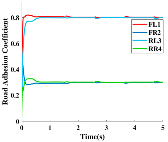
Figure 4.
100 km/h open road: RAC for each wheel.
- (2)
- Scenario 2: Joint Road
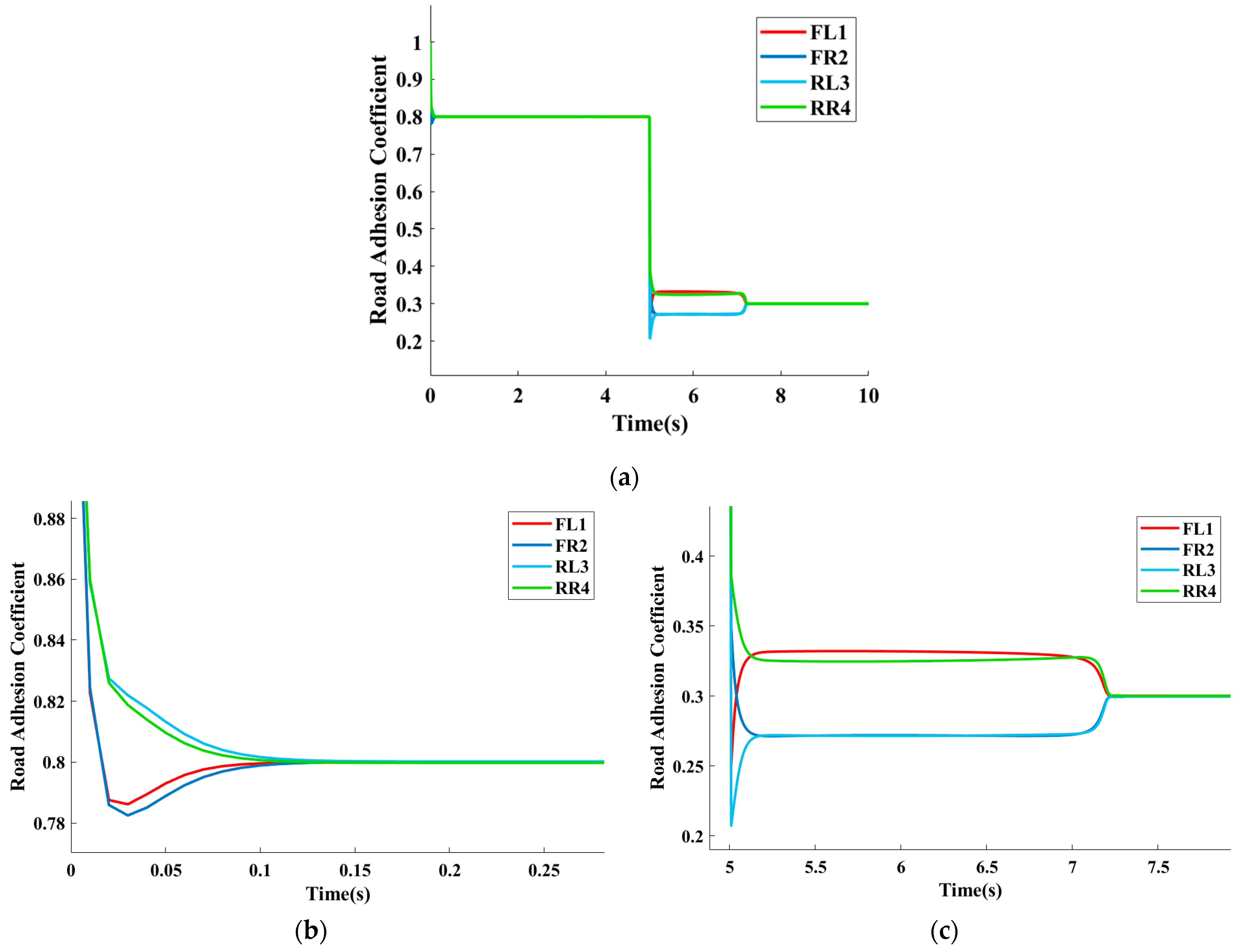
To verify the algorithm’s estimation accuracy under sudden changes in the road adhesion coefficients, in Carsim, the VS was maintained at 100 km/h, with the RACs set to 0.8 and 0.3 for the joint road. The steering angle was set to the sinusoidal input, similar to the open road scenario. The simulation results are shown in Figure 5. The adhesion coefficients of four wheels quickly converged to 0.8. Around 5 s, the vehicle transitioned from a high RAC to a low RAC. Each wheel showed a brief fluctuation and then quickly stabilized and converged to 0.3, indicating the UKF algorithm’s good response performance to sudden changes in the road conditions.
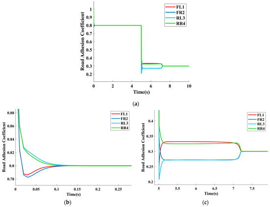
Figure 5.
100 km/h jointed road: (a) RAC for each wheel; (b) 0.8 RAC and (c) 0.3 RAC.
4. Path-Tracking Control Strategy Based on LLCC
4.1. Overall Path-Tracking Control Strategy Design
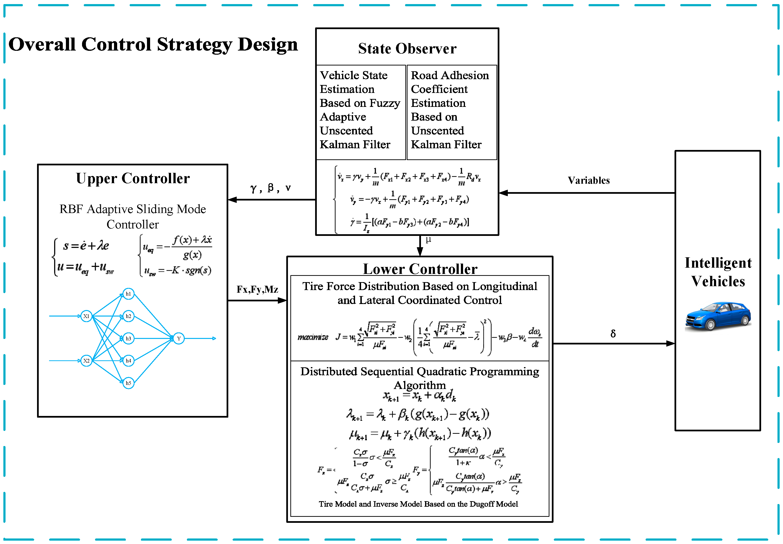
This study adopted a layered control structure to design the path-tracking controller. The upper-level controller uses an adaptive sliding mode controller based on RBF neural networks, with the desired vehicle speed, yaw rate, and sideslip angle as control objectives. The sliding mode controller was employed to calculate the desired longitudinal force, the lateral force, and the yaw moment of the vehicle, achieving the decoupling of these forces and moments. The lower-level controller targets the distribution of the tire longitudinal and lateral forces and considers the coupling between tire forces and load transfer. The UKF road adhesion coefficient observer was used to calculate the road adhesion coefficient for each tire in real time. To improve vehicle stability under complex conditions, the optimization objective was set to minimize the utilization of tire-adhesion coefficients. The desired vehicle longitudinal force, lateral force, and yaw moment were used as equality constraints. The DSQP algorithm calculated the longitudinal forces for all four wheels and the lateral forces for the front axle, achieving path-tracking control under complex conditions. The overall control framework is shown in Figure 6.
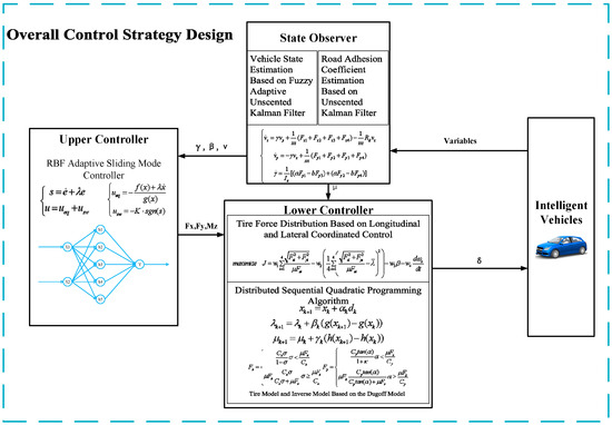
Figure 6.
Overall control strategy.
4.2. Design and Optimization of Path-Tracking Controller under RBF Neural Networks
In the path-tracking control of intelligent vehicles, considering the adaptability and the robustness of SMC and the approximation capability of RBF neural networks, this paper designs an ASMC under RBF neural networks. This controller aims to solve the decoupling control problem of vehicle longitudinal, lateral, and yaw motions, enhancing adaptability to uncertainties and external disturbances.
The SMC controls the system’s state variables by designing a sliding surface, ensuring the system’s robustness as it moves along the sliding surface. It is as follows:
where is the error between system state variables and reference values, and is the control parameter. Control law is defined as follows:
The equivalent control term is used to track the sliding surface, while the switching control term is used to keep the system state on the sliding surface. The specific equivalent control term is determined by the following equation:
where is the nonlinear dynamic part, and is the input matrix. The equivalent control term ensures that, under ideal conditions, the system state can slide along the sliding surface.
The switching control term is designed as follows:
where is the control gain, and the function ensures that the system state switches on the sliding surface. However, since sign function can cause chattering, a hyperbolic tangent function is usually adopted in practical applications to reduce chattering:
where is the boundary layer thickness parameter, adjusting width to reduce chattering.
The adaptive sliding mode controller uses the approximation capability of RBF neural networks to compensate for system uncertainties and external disturbances, thus improving the control system’s adaptability.
An RBF neural network consists of an input layer, a hidden layer, and an output layer. The activation function of the hidden layer is a Gaussian function, and the network output is defined as follows:
where are the network weights, are the Gaussian activation functions, and is the number of hidden layer nodes. The Gaussian function is expressed as follows:
where is the center of the node, and is its width parameter.
To ensure that the RBF neural network can approximate system uncertainties in real time, an adaptive algorithm is used to adjust the network weights. The specific adaptive law is as follows:
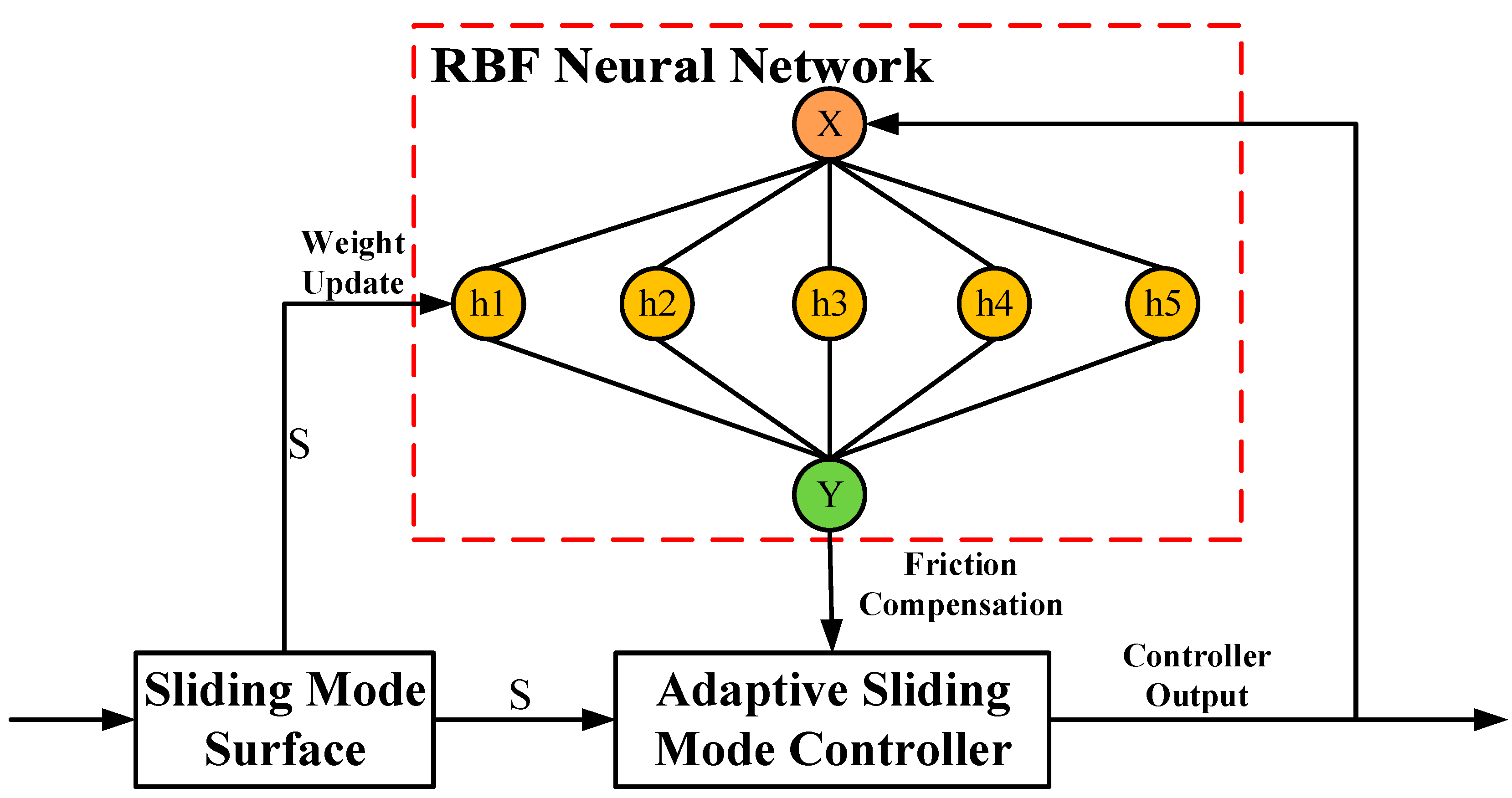
where is the learning rate, ensuring that the network weights can be quickly adjusted near the sliding surface. Through adaptive adjustment, the RBF neural network can approximate the unknown parts of the system in real time, improving the controller’s adaptability and robustness. The structural design of the controller is shown in Figure 7.
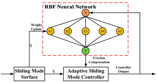
Figure 7.
RBF Neural Network-Based ASMC.
4.3. Tire Force Distribution under the Longitudinal and Lateral Coordinated Control
4.3.1. Selection of Optimization Objectives
In the optimization of tire force distribution under longitudinal and lateral coordinated control, the optimization objectives should encompass maximizing the utilization rate of adhesion coefficients for all four tires, ensuring balanced tire utilization, and improving vehicle stability and handling performance. Specifically, the optimization objectives include maximizing the utilization rate of adhesion coefficients, minimizing the variance of adhesion coefficient utilization rates, enhancing the stability of the yaw rate response, and reducing the vehicle’s sideslip angle. These objectives can be integrated into a multi-objective optimization function, balancing the influence of each objective through a weighted summation.
The multi-objective optimization function is as follows:
where is the average utilization rate of the RAC of four tires, is the vehicle’s sideslip angle, and , , , are weight coefficients that adjust the weights of each objective based on actual requirements. The variables and constraints in this optimization function relate to real-world performance metrics such as tire-adhesion utilization, side-slip angle, and yaw rate. The choice of weight coefficients in the optimization reflects the importance of each objective under different driving conditions, ensuring that the vehicle performs optimally across various scenarios.
During the optimization process, it is necessary to consider dynamic constraints to ensure that the longitudinal and lateral forces remain within the tire-adhesion limits, while also satisfying the vehicle dynamics balance conditions and restricting tire forces from exceeding their maximum values. Ultimately, this optimization method can achieve the optimal utilization rate of tire-adhesion coefficients under different working conditions, thereby enhancing vehicle’s stability.
4.3.2. Establishment of Constraints
In vehicle dynamics control, the upper-level controller usually calculates target longitudinal force, the lateral force, and the yaw moment to achieve the vehicle’s desired motion state. These target forces are the expected values of the vehicle’s actual operation and need to be achieved through the reasonable distribution of tire forces. The tracking constraints of the target forces ensure that the optimization of the tire force distribution can achieve the dynamic targets set by the upper-level controller.
Specifically, the target longitudinal force represents the vehicle’s acceleration or deceleration requirement in longitudinal direction. The target lateral force reflects the vehicle’s lateral stability requirement during steering. The target yaw moment is used to control the vehicle’s yaw rate, ensuring that the vehicle can follow the desired trajectory. The tracking constraints of these target forces can be expressed as follows:
where and are longitudinal, lateral distances from tire to the vehicle’s center of mass, respectively. These constraints ensure that the calculated tire forces during tire force distribution optimization can achieve the vehicle’s desired motion state.
The tire force constraints are based on the maximum adhesion force limit of tires, ensuring that the tire forces in the longitudinal and lateral directions do not exceed their physical limits. The combined force of the tire’s longitudinal force and lateral force should not exceed the tire’s maximum adhesion force . This constraint can be expressed as follows:
This constraint considers the nonlinear adhesion characteristics of the tires, ensuring that the tires maintain a stable grip under extreme conditions. This prevents the tires from losing adhesion under excessive longitudinal or lateral forces, which could lead to vehicle instability. Additionally, the tire force constraints need to satisfy the following physical limits:
Vehicle dynamics constraints mainly include the longitudinal force balance, the lateral force balance, and the yaw moment balance, reflecting the vehicle’s dynamic behavior in various directions. These constraints can be expressed as follows:
By comprehensively considering the above dynamics constraints, the optimization of tire force distribution not only achieves the tracking of target forces but also ensures vehicle stability and safety under various dynamic conditions.
4.3.3. Optimal Tire Force Calculation Based on Distributed Sequential Quadratic Programming Algorithm
DSQP is a method used to solve large-scale nonlinear optimization problems. By decomposing the original problem into a series of smaller sub-problems for iterative solving, DSQP is mainly applied to optimization problems with complex structures, such as multi-objective optimization and constrained optimization.
The DSQP algorithm is applied to optimize tire force distribution in real time, ensuring that the vehicle maintains stability while minimizing tire wear and maximizing traction. The constraints in this optimization problem are directly related to the vehicle’s physical limitations and operational conditions. Consider the general form of a nonlinear optimization problem:
where is the decision variable, is the objective function, is the equality constraint, and is the inequality constraint. Here, the equality constraints and inequality constraints are represented as follows:
DSQP decomposes the large-scale problem into multiple sub-problems to be solved in parallel, with each sub-problem corresponding to a sub-domain:
Here, is the decision variable of the sub-problem, is the corresponding sub-objective function, and and are the corresponding sub-constraints.
In each iteration step, the quadratic programming sub-problems for each sub-problem are solved:
The above sub-problems are solved by linearization and quadratic approximation. The step direction for each sub-problem is adjusted through the second-order derivative of the local Lagrange function.
At the end of each iteration, the global variables and Lagrange multipliers are updated through a coordination mechanism, and these updates are passed to each sub-problem:
where , , are step size parameters. These parameters control the update step sizes, ensuring the convergence of the algorithm. In particular, the update of global variables x needs to comprehensively consider the step directions of all sub-problems.
5. Simulation Analysis of Path-Tracking Control System
5.1. Simulation Analysis of Controller Optimization Strategy
In the field of intelligent vehicle control, SMC and ASMC are widely used for path tracking. This study conducted simulation analysis to compare the performance of SMC and ASMC under different conditions, exploring their optimization strategies.
In Carsim, the VS was maintained at 54 km/h, and the RAC was 0.85. The simulation scenario selected was the typical double lane change scenario to evaluate the dynamic response performance of vehicles under complex conditions. Under the initial conditions, the vehicle’s SA and YR were both set to 0 to ensure stability and consistency of the simulation. The simulation results can be seen in Figure 8.
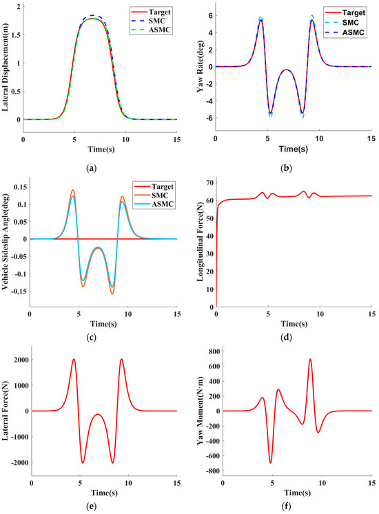
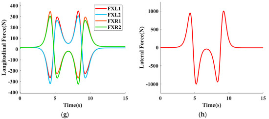
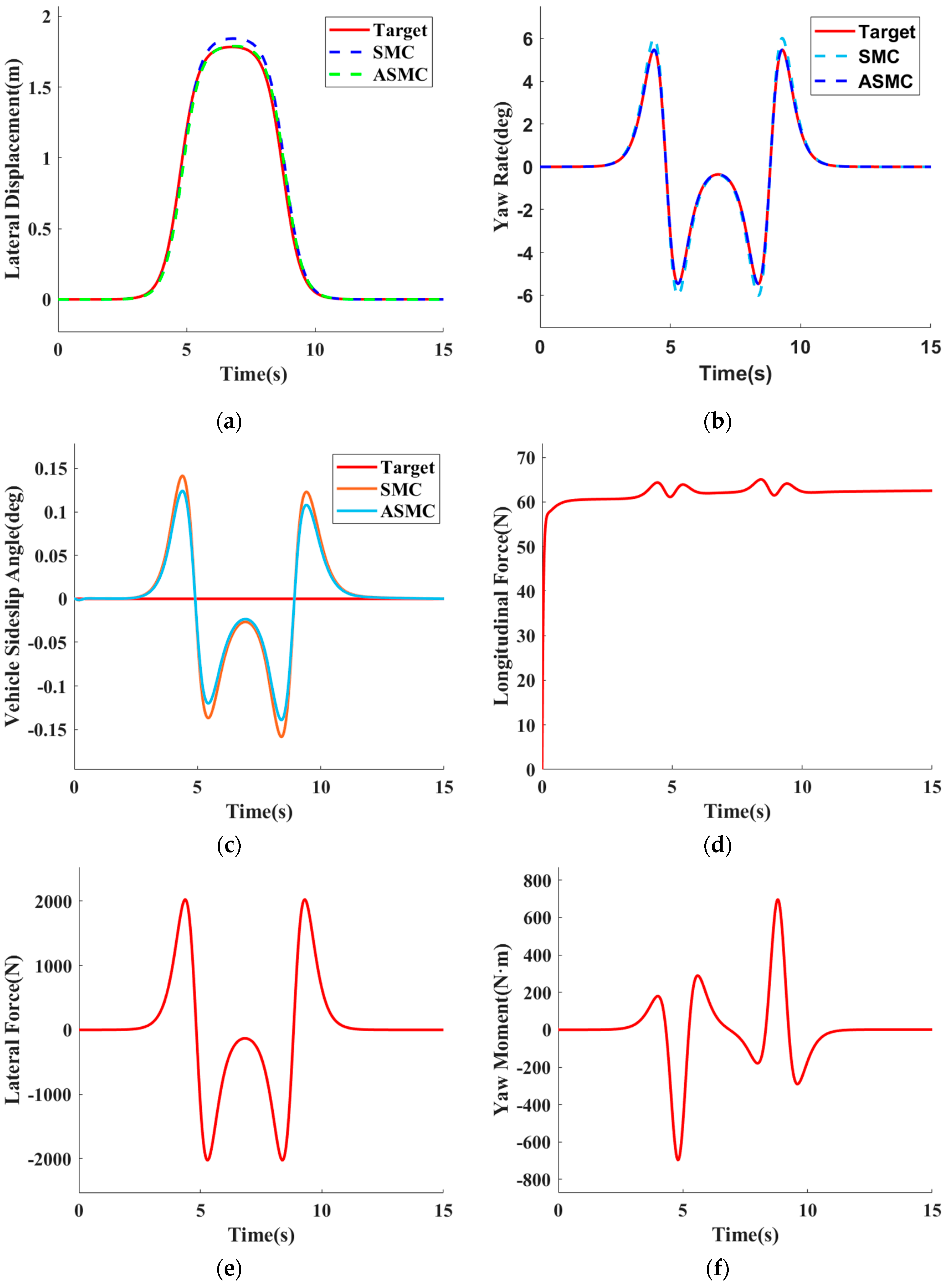
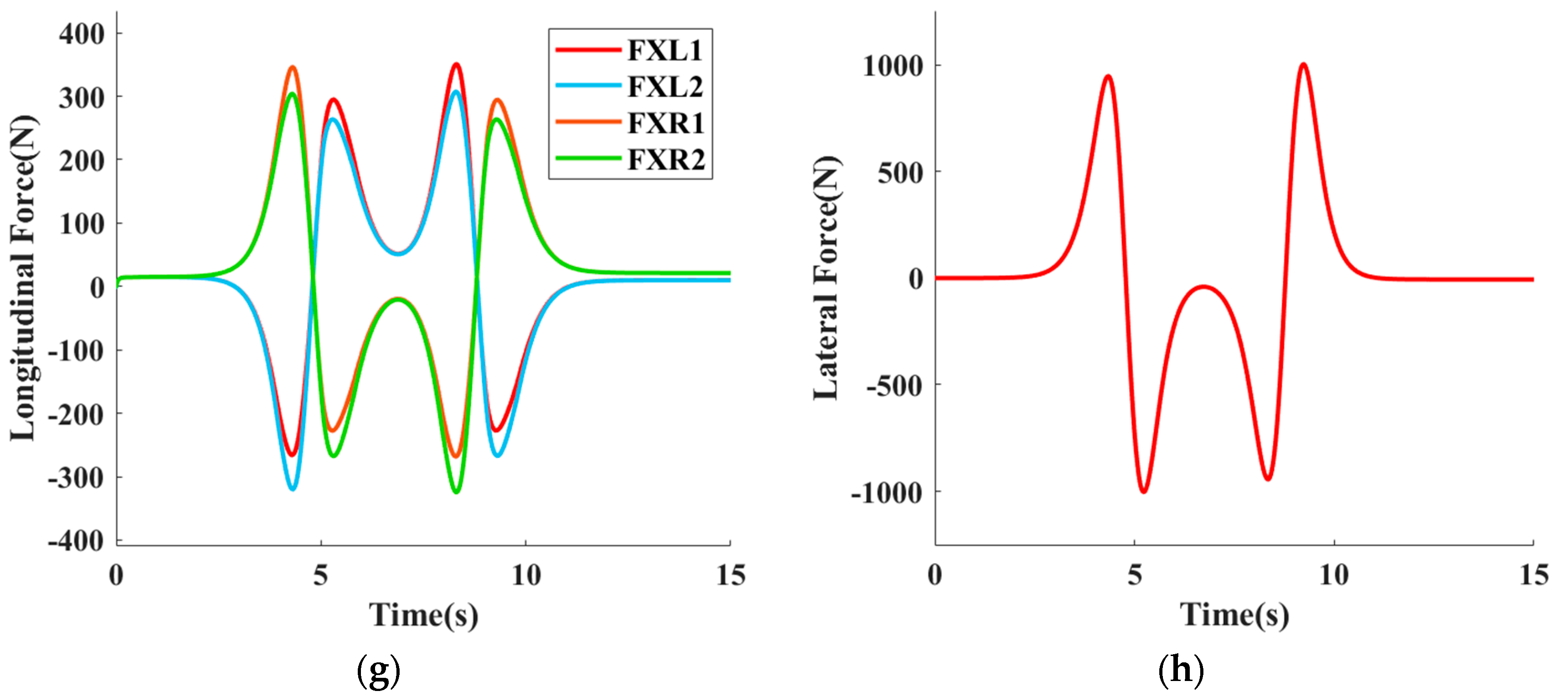
Figure 8.
Comparison of simulation results between SMC and ASMC: (a) comparison of tracking trajectories; (b) YR; (c) SA; (d) longitudinal force (LF); (e) lateral force (LAF); (f) yaw moment (YM); (g) longitudinal tire force (LTF) and (h) front axle lateral force (FALF).
The simulation comparison between SMC and ASMC shows that ASMC outperforms traditional SMC in terms of control accuracy, system stability, and chattering suppression. The tracking trajectory comparison (Figure 8a) indicates that ASMC provides higher tracking accuracy in path tracking, especially during the peak displacement period between 5 and 10 s. ASMC offers more accurate tracking, significantly reducing tracking errors while effectively minimizing the chattering phenomenon in ASMC, resulting in smoother control inputs. The yaw rate (Figure 8b) shows that ASMC provides better response speed and stability during the peak yaw rate periods at 5 and 10 s. In the sideslip angle (Figure 8c), both control strategies keep the sideslip angle within an acceptable range, but ASMC performs better in minimizing deviation from the target angle. The LF (Figure 8d) demonstrates consistent and stable longitudinal force throughout the simulation, with minimal fluctuation around 60 N. The LAF (Figure 8e), YM (Figure 8f), LTF (Figure 8g), and FALF (Figure 8h) show that ASMC has fewer peak yaw moments and more balanced force distribution among the wheels, allowing for quick and stable output and better adaptability to dynamic vehicle control. The results indicate that ASMC outperforms traditional SMC in terms of tracking accuracy, stability, and robustness.
In Table 1, a significant difference is shown in tracking errors between SMC and ASMC. The data in the table show that the maximum error of ASMC is 0.0677, which is significantly lower than the maximum error of SMC, which is 0.0912. This indicates that ASMC has better control accuracy than SMC. Additionally, the average error of ASMC is only 0.0014, which is also significantly lower than the average error of SMC, which is 0.0155. These data suggest that ASMC not only effectively reduces the maximum error in practical applications but also significantly lowers the average error, improving overall tracking performance of the system.

Table 1.
Comparison of errors between SMC and ASMC.
5.2. Simulation Analysis of LLCC Strategy
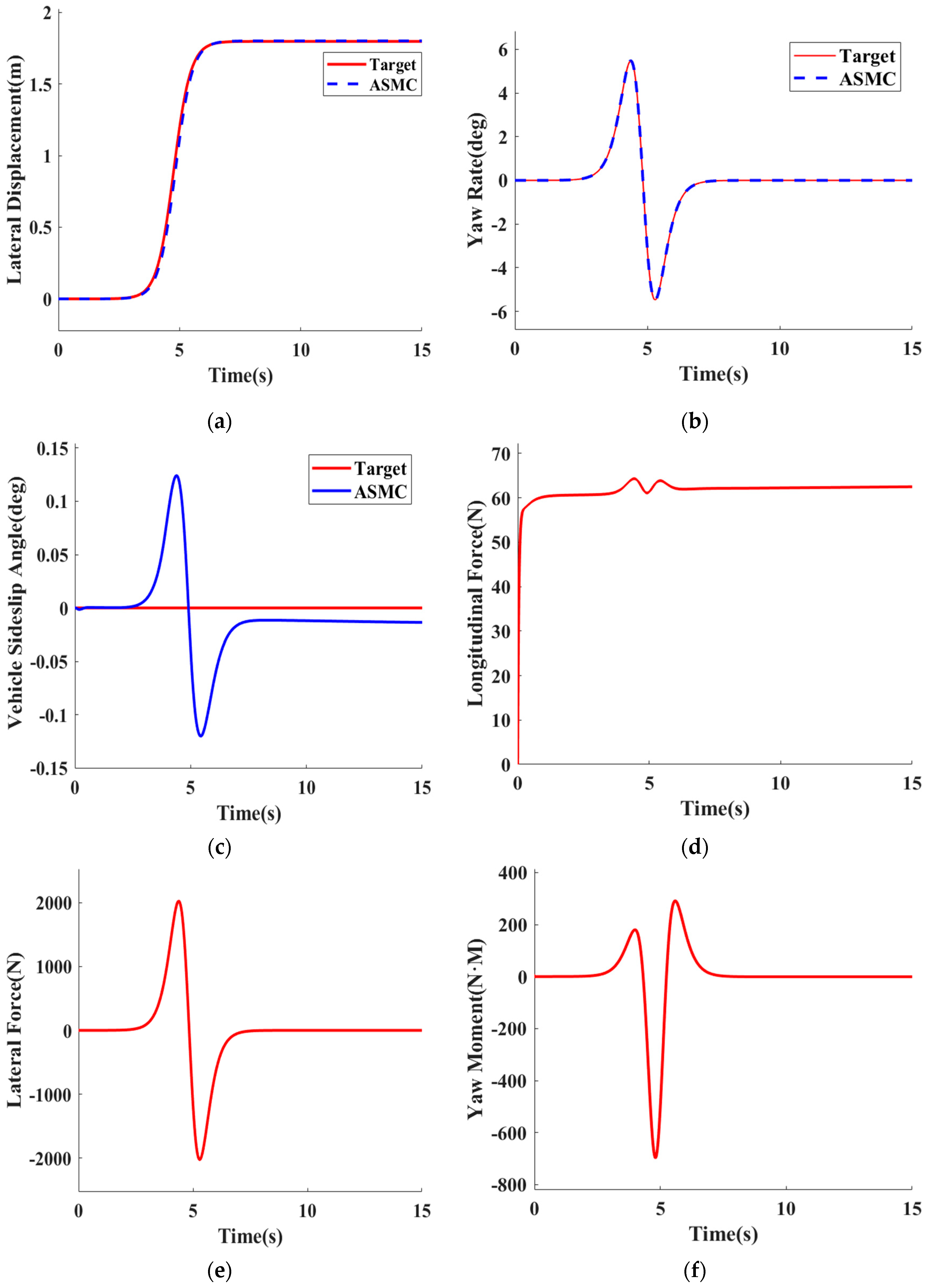
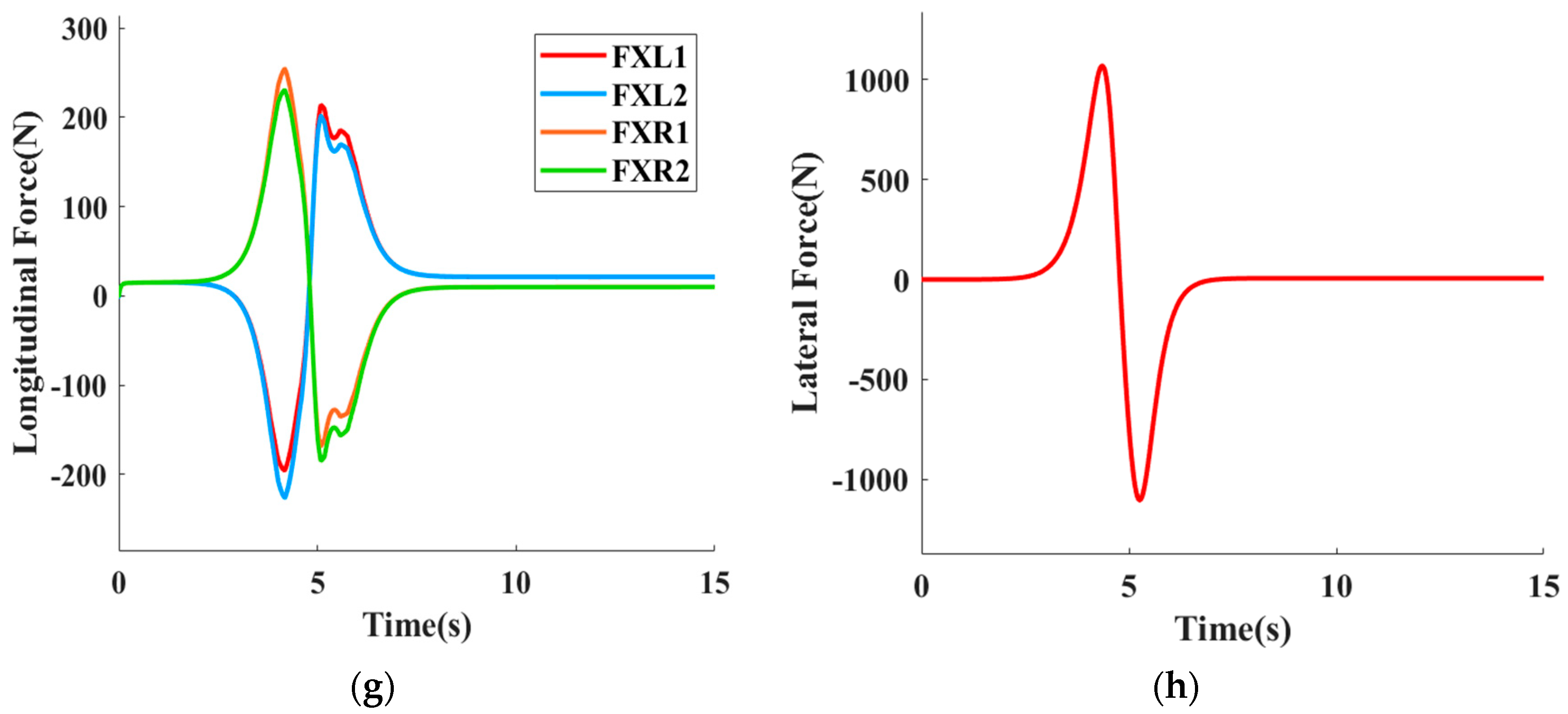
5.2.1. DLC on Low RAC
To verify the control performance of ASMC under complex conditions, VS was adjusted to 54 km/h and the RAC was configured to 0.3 in Carsim. Low-adhesion road surfaces caused tires to enter the nonlinear region more easily, leading to vehicle instability. The simulation results are shown in Figure 9.
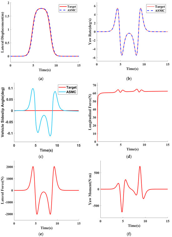
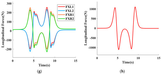
Figure 9.
DLC on low adhesion surface (a) comparison of tracking trajectories; (b) YR; (c) SA; (d) LF; (e) LAF; (f) YM; (g) LTF and (h) FALF.
Based on the simulation results of ASMC under DLC low RAC, conclusions can be drawn. Figure 9a shows that ASMC closely follows the reference trajectory during the peak displacement period between 5 and 10 s, significantly reducing tracking errors and providing smoother control inputs. Figure 9b indicates that ASMC has better response speed and stability during the peak yaw rate periods at 5 and 10 s, with the yaw rate closely aligned with the target value. In Figure 9c, ASMC performs better in minimizing deviation from the target angle, thereby improving the lateral stability and the handling performance. Figure 9d demonstrates that ASMC maintains stable and consistent longitudinal force output throughout the simulation, with minimal fluctuation around 60 N, which helps to maintain the vehicle speed and trajectory accuracy. Figure 9e shows that ASMC maintains stable and consistent lateral control forces, adapting to road surface changes and maintaining vehicle stability. Figure 9f indicates that ASMC has fewer peak yaw moments, resulting in smoother and more stable yaw motion, enhancing overall vehicle stability. Figure 9g illustrates that ASMC’s coordinated output of longitudinal tire forces shows balanced force distribution, which is crucial for maintaining tire traction and stability under low-adhesion conditions. Figure 9h demonstrates that ASMC effectively controls the front axle lateral force output, quickly responding to changes and maintaining stability, ensuring maneuverability and vehicle dynamics performance during lane changes.
5.2.2. Lane Change on High RAC
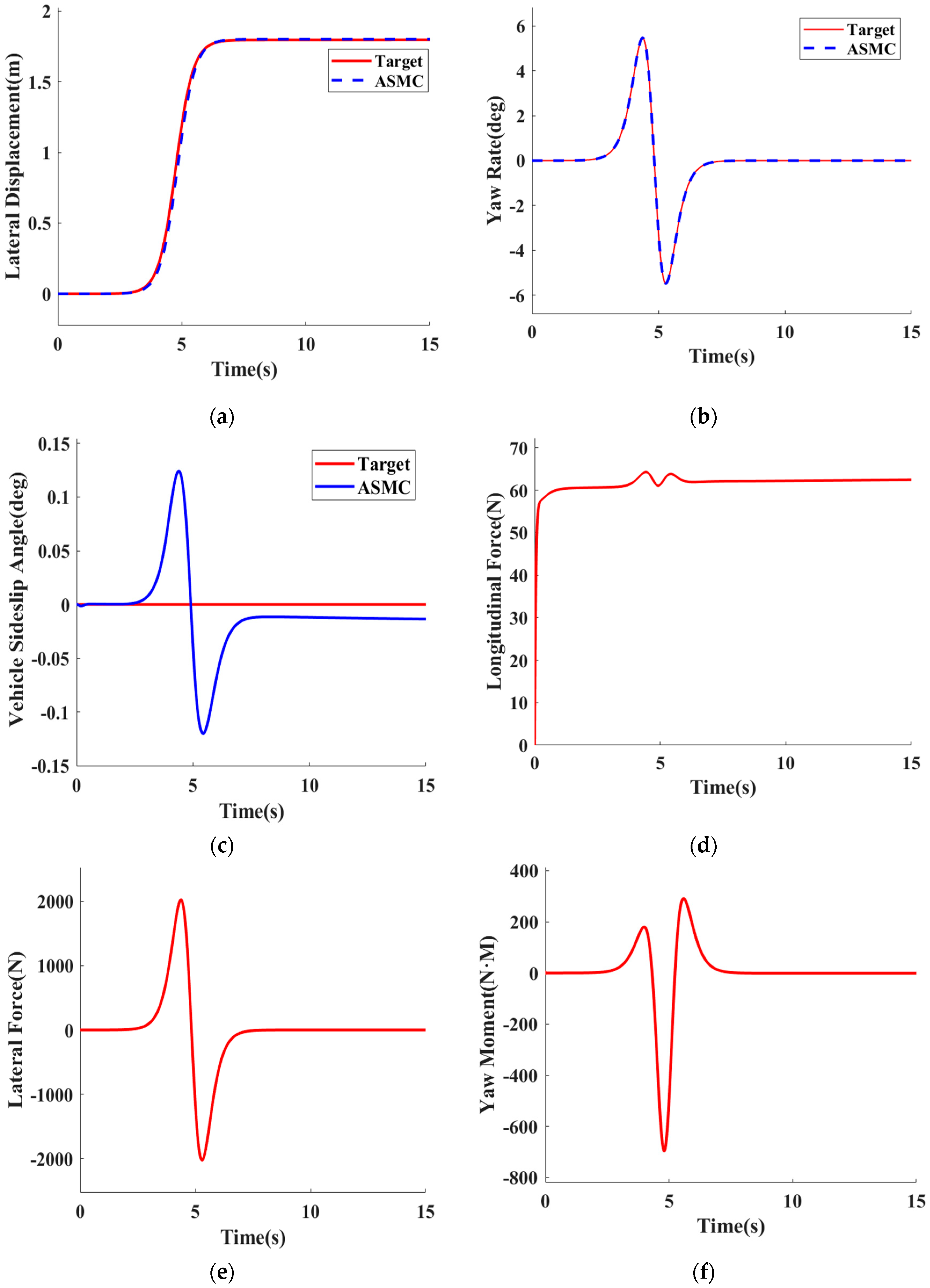
High-adhesion road surfaces provide a relatively uniform high-adhesion surface, making vehicle movement more stable and predictable. The path-tracking controller’s performance needs to be rigorously tested to ensure it can provide efficient and reliable control under various real driving conditions. In the Carsim simulation environment, the VS was maintained at 54 km/h, and the RAC was 0.85 to simulate typical road conditions in real driving environments. The simulation results are shown in Figure 10.
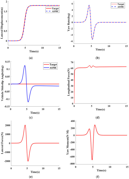

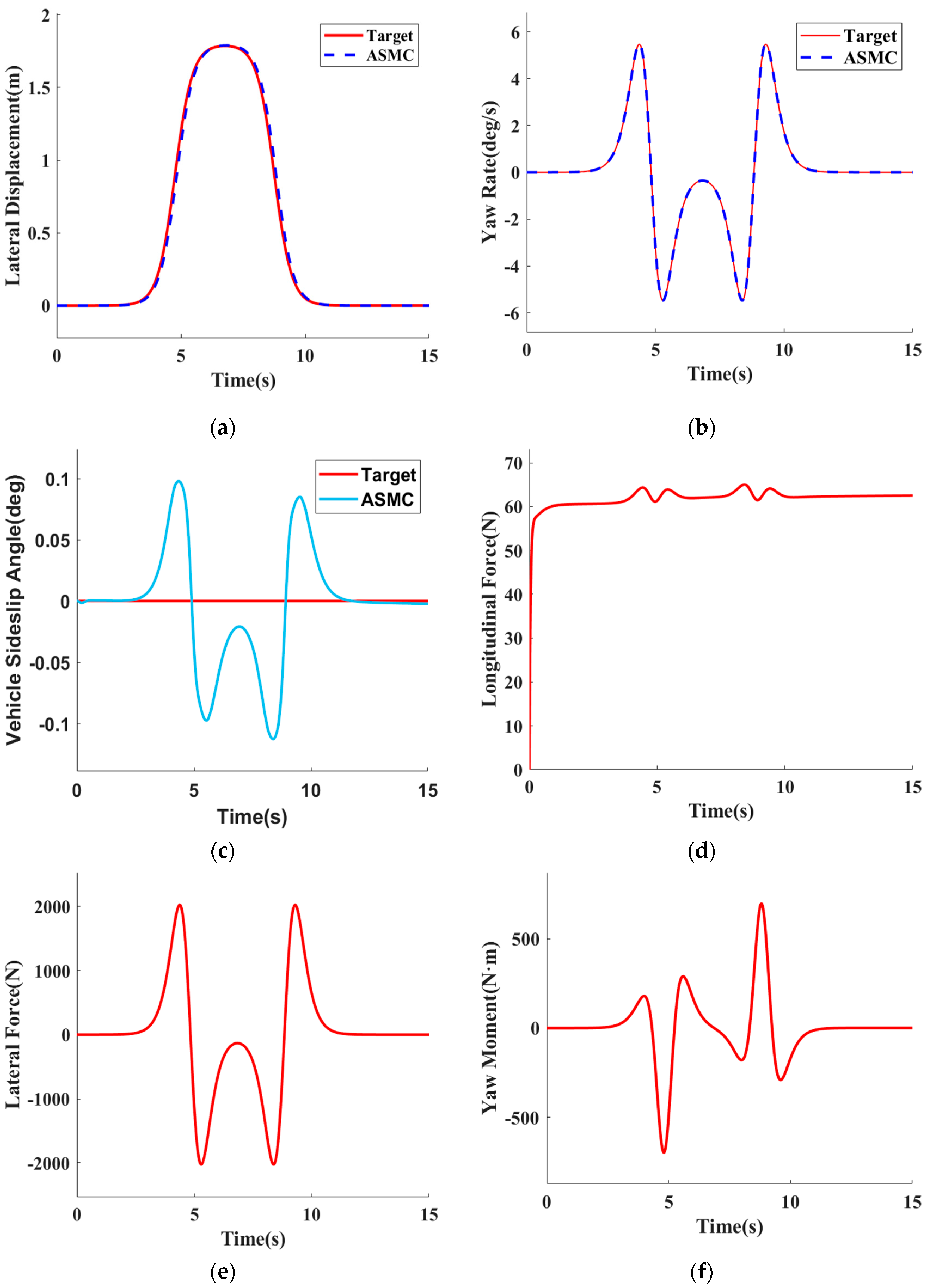
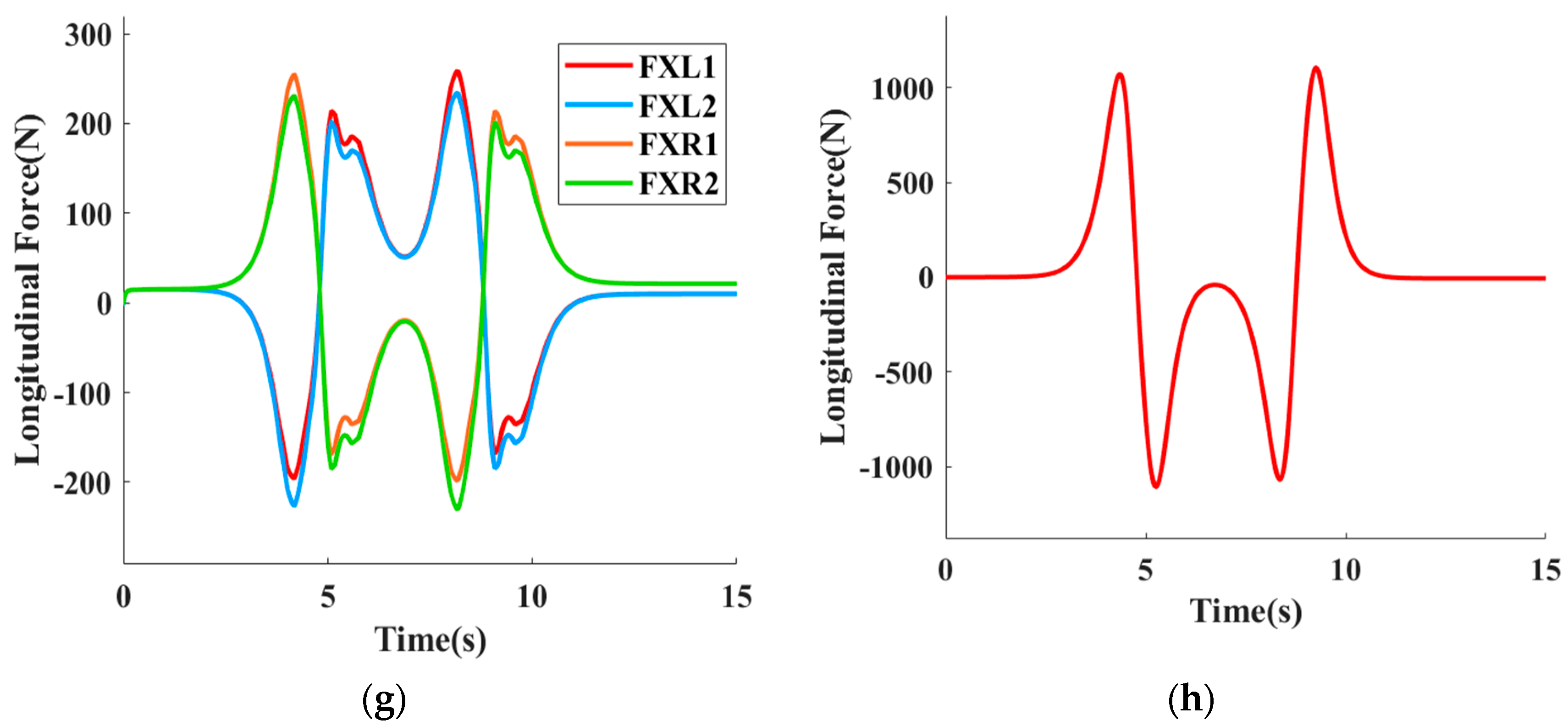
Figure 10.
Lane change on high RAC (a) comparison of tracking trajectories; (b) YR; (c) SA; (d) LF; (e) LAF; (f) YM; (g) LTF and (h) FALF.
Based on the results of ASMC during a lane change with a high RAC, conclusions can be drawn. Figure 10a shows that ASMC can precisely track the target lateral displacement, ensuring the vehicle reaches the 2-m target position within approximately 5 s. The yaw rate response in Figure 10b exhibits good regulation, with minor oscillations during the lane change process that are quickly suppressed. Figure 10c reflects the lateral stability of the vehicle under ASMC control, with transient oscillations rapidly decaying and maintaining the target sideslip angle close to zero. In Figure 10d, the longitudinal force peaks during the critical phase of the lane change and quickly returns to balance, demonstrating ASMC’s effective management of dynamic adjustments. The lateral force responses in Figure 10e,h show significant transient peaks at around 5 s, indicating that ASMC can effectively respond to sudden changes in lateral dynamics. The yaw moment response in Figure 10f also shows significant peaks during the lane change, followed by rapid stabilization, ensuring directional stability of the vehicle. Figure 10g displays the distribution of longitudinal forces across the wheels, where ASMC ensures balanced force distribution, contributing to traction and stability during the lane change.
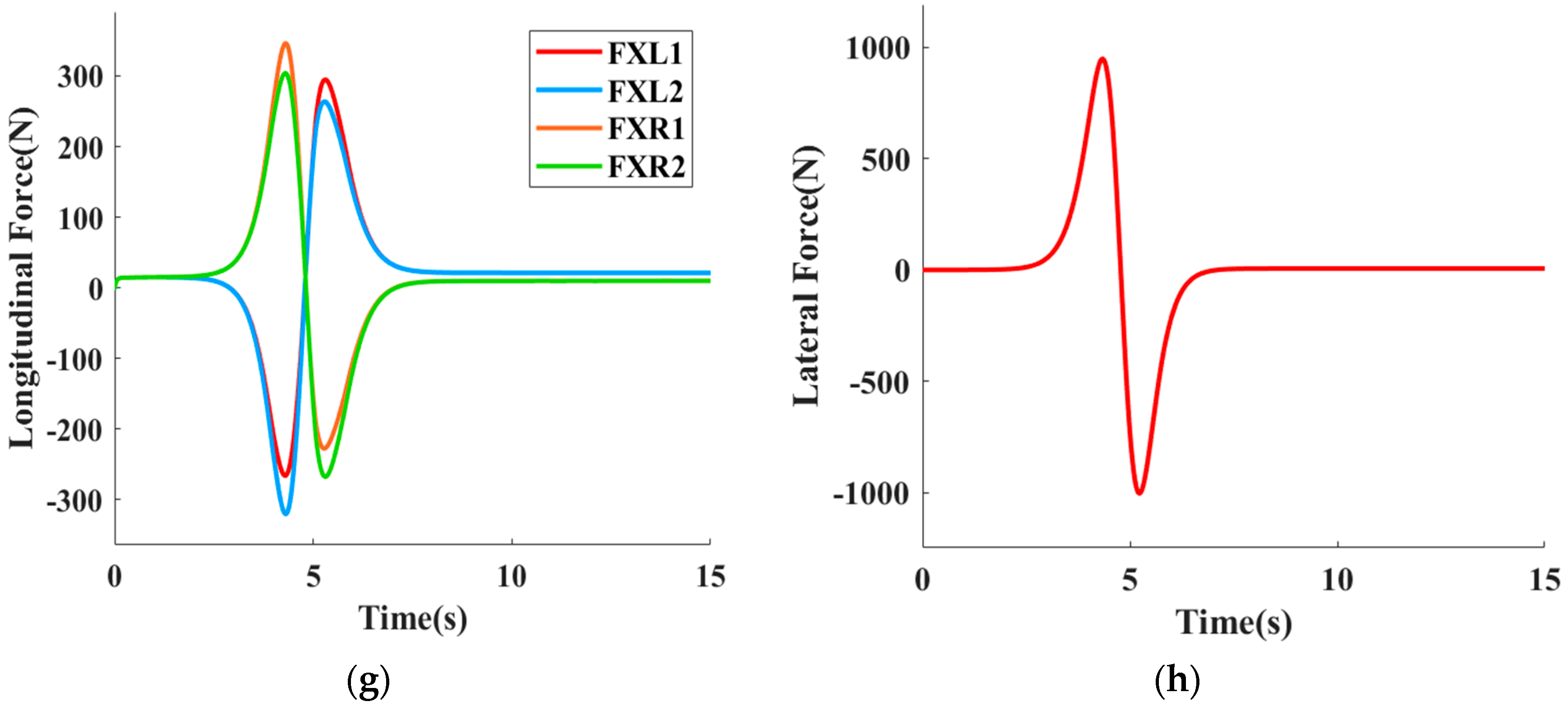
5.2.3. Lane Change on Low RAC
To verify control performance of ASMC under complex conditions, the VS was maintained at 54 km/h, and the RAC was 0.85 in Carsim. Low-adhesion road surfaces, as a type of complex condition, cause tires to enter the nonlinear region more easily, leading to vehicle instability. The simulation results are shown in Figure 11.
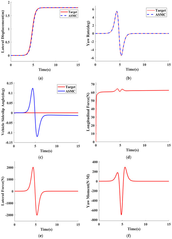
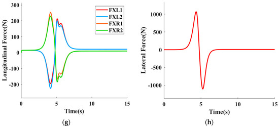
Figure 11.
Lane change on low RAC (a) comparison of tracking trajectories; (b) YR; (c) SA; (d) LF; (e) LAF; (f) YM; (g) LTF and (h) FALF.
Based on the results of ASMC during a lane change with a low RAC, conclusions can be drawn. Figure 11a shows that ASMC can effectively track the target lateral displacement, reaching the target 2-m lateral displacement within approximately 5 s, despite the vehicle’s instability on low-adhesion surfaces. The yaw rate response in Figure 11b exhibits significant transient oscillations, peaking at around 5 s during the lane change, then quickly decaying to zero, indicating that ASMC effectively regulates the yaw rate to return to stability. Figure 11c demonstrates that on low-adhesion surfaces, the vehicle’s sideslip angle experiences large transient fluctuations, peaking at around 5 s. However, ASMC can quickly bring the sideslip angle back to near zero, maintaining the vehicle’s lateral stability. The longitudinal force in Figure 11d shows minor fluctuations during the lane change, peaking at around 5 s and then gradually returning to balance. This indicates that ASMC effectively adjusts the longitudinal force to maintain stable driving. The lateral force response in Figure 11e shows significant transient peaks, reaching a maximum at around 5 s and then quickly returning to zero. The yaw moment in Figure 11f also exhibits significant transient peaks during the lane change, peaking at around 5 s and then rapidly decaying to zero. Figure 11g illustrates that all of the wheels’ longitudinal forces experience noticeable fluctuations during the lane change, especially peaking at around 5 s before returning to balance. The front axle wheels’ lateral force in Figure 11h shows significant transient peaks, reaching a maximum at around 5 s and then quickly returning to zero. These results demonstrate that ASMC exhibits excellent control performance and stability under low-adhesion lane change conditions. Despite the increased instability on low-adhesion surfaces, ASMC can effectively adjust vehicle dynamics parameters, ensuring safety and reliability under complex conditions.
6. Conclusions
To address the issues of tracking accuracy degradation and vehicle instability caused by longitudinal and lateral coupling constraints and model uncertainties in intelligent vehicle path-tracking control, a LLCC strategy optimized based on ASMC was proposed. First, to improve the path-tracking accuracy and stability of intelligent vehicles under complex conditions, a fuzzy adaptive unscented Kalman filter state observer was designed to estimate VS, YR, and SA in real time. Additionally, a RAC observer based on the UKF was designed to estimate the RAC in real time. Next, the upper-level controller was designed with an ASMC based on RBF neural networks. By combining SMC and neural network technology, the controller can effectively handle system disturbances and uncertainties, enhancing the adaptability and robustness of the controller. The lower-level controller decouples the longitudinal and lateral forces of the vehicle and optimizes tire force distribution to improve path-tracking performance under complex conditions. Finally, the effectiveness of the proposed optimized control strategy was validated using Carsim and Matlab/Simulink software. The results show that the designed control strategy optimized with ASMC can adaptively adjust control parameters to accommodate various driving conditions, ensuring tracking accuracy and stability of the vehicle under different adhesion coefficients and driving conditions.
Author Contributions
Y.W.: Writing—review and editing. Z.W.: Writing—original draft, methodology and Visualization. D.S.: Writing—review and editing, Supervision, Project administration. F.C.: Conceptualization, Visualization. J.G.: Writing—review and editing. J.W.: Writing—review and editing, Supervision. All authors have read and agreed to the published version of the manuscript.
Funding
This research was supported by the special task project fund of Project for Humanities and Social Sciences in Universities of Hubei Province (2024JDB07), the Hubei Provincial Department of Education (23Q177), the 2024 “Xiangjiang Policy Discussion” Key Project of the Xiangyang Federation of Social Sciences and the Xiangyang Cultural Xiangyang Research Association (WHXYZDKT202401), and the Hubei Key Laboratory of Power System Design and Test for Electrical Vehicle (ZDSYS202412).
Data Availability Statement
The raw data supporting the conclusions of this article will be made available by the authors on request.
Conflicts of Interest
The authors declare no competing interests.
References
- Miao, H.; Diao, P.; Xu, G.; Yao, W.; Song, Z.; Wang, W. Research on decoupling control for the longitudinal and lateral dynamics of a tractor considering steering delay. Sci. Rep. 2022, 12, 13997. [Google Scholar] [CrossRef] [PubMed]
- Li, Y.; Hao, G. Energy-optimal adaptive control based on model predictive control. Sensors 2023, 23, 4568. [Google Scholar] [CrossRef] [PubMed]
- Feng, X.; Liu, S.; Yuan, Q.; Xiao, J.; Zhao, D. Research on wheel-legged robot based on LQR and ADRC. Sci. Rep. 2023, 13, 15122. [Google Scholar] [CrossRef] [PubMed]
- Wu, L.; Zhou, R.; Bao, J.; Yang, G.; Sun, F.; Xu, F.; Jin, J.; Zhang, Q.; Jiang, W.; Zhang, X. Vehicle stability analysis under extreme operating conditions based on LQR control. Sensors 2022, 22, 9791. [Google Scholar] [CrossRef]
- Ji, X.; Ding, S.; Wei, X.; Mei, K.; Cui, B.; Sun, J. Path Tracking Control of Unmanned Agricultural Tractors via Modified Supertwisting Sliding Mode and Disturbance Observer. IEEE/ASME Trans. Mechatron. 2024. [Google Scholar] [CrossRef]
- Oh, K.; Seo, J. Development of a sliding-mode-control-based path-tracking algorithm with model-free adaptive feedback action for autonomous vehicles. Sensors 2022, 23, 405. [Google Scholar] [CrossRef] [PubMed]
- Rickenbach, R.; Köhler, J.; Scampicchio, A.; Zeilinger, M.N.; Carron, A. Active learning-based model predictive coverage control. IEEE Trans. Autom. Control 2024. [Google Scholar] [CrossRef]
- Xu, S.; Peng, H. Design, analysis, and experiments of preview path tracking control for autonomous vehicles. IEEE Trans. Intell. Transp. Syst. 2019, 21, 48–58. [Google Scholar] [CrossRef]
- Ma, Y.; Duan, P.; Sun, Y.; Chen, H. Equalization of lithium-ion battery pack based on fuzzy logic control in electric vehicle. IEEE Trans. Ind. Electron. 2018, 65, 6762–6771. [Google Scholar] [CrossRef]
- Yao, M.; Deng, H.; Feng, X.; Li, P.; Li, Y.; Liu, H. Improved dynamic windows approach based on energy consumption management and fuzzy logic control for local path planning of mobile robots. Comput. Ind. Eng. 2024, 187, 109767. [Google Scholar] [CrossRef]
- He, Y.; Liu, Y.; Yang, L.; Qu, X. Deep adaptive control: Deep reinforcement learning-based adaptive vehicle trajectory control algorithms for different risk levels. IEEE Trans. Intell. Veh. 2023, 9, 1654–1666. [Google Scholar] [CrossRef]
- Jiang, Y.; Meng, H.; Chen, G.; Yang, C.; Xu, X.; Zhang, L.; Xu, H. Differential-steering based path tracking control and energy-saving torque distribution strategy of 6WID unmanned ground vehicle. Energy 2022, 254, 124209. [Google Scholar] [CrossRef]
- Kim, H.; Wan, W.; Hovakimyan, N.; Sha, L.; Voulgaris, P. Robust vehicle lane keeping control with networked proactive adaptation. Artif. Intell. 2023, 325, 104020. [Google Scholar] [CrossRef]
- Li, H.; Huang, J.; Yang, Z.; Hu, Z.; Yang, D.; Zhong, Z. Adaptive robust path tracking control for autonomous vehicles with measurement noise. Int. J. Robust Nonlinear Control 2022, 32, 7319–7335. [Google Scholar] [CrossRef]
- Yang, C.; Liu, J. Trajectory tracking control of intelligent driving vehicles based on MPC and Fuzzy PID. Math. Probl. Eng. 2023, 2023, 2464254. [Google Scholar] [CrossRef]
- Li, G.; Shang, P.; Zheng, C.; Sun, D. A Lateral Control Method of Intelligent Vehicles Based on Shared Control. Symmetry 2022, 14, 2447. [Google Scholar] [CrossRef]
- Chu, X.; Liu, Z.; Mao, L.; Jin, X.; Peng, Z.; Wen, G. Robust event triggered control for lateral dynamics of intelligent vehicle with designable inter-event times. IEEE Trans. Circuits Syst. II Express Briefs 2022, 69, 4349–4353. [Google Scholar] [CrossRef]
- El Hajjami, L.; Mellouli, E.M.; Žuraulis, V.; Berrada, M.; Boumhidi, I. A robust intelligent controller for autonomous ground vehicle longitudinal dynamics. Appl. Sci. 2022, 13, 501. [Google Scholar] [CrossRef]
- Yang, D.; Liu, T.; Song, D.; Zhang, X.; Zeng, X. A real time multi-objective optimization Guided-MPC strategy for power-split hybrid electric bus based on velocity prediction. Energy 2023, 276, 127583. [Google Scholar] [CrossRef]
- Zhou, Y.; Pan, M.; Guan, W.; Cao, X.; Chen, H.; Yuan, L. A Novel Longitudinal Control Method Integrating Driving Style and Slope Prediction for High-Efficiency HD Vehicles. Appl. Sci. 2023, 13, 11968. [Google Scholar] [CrossRef]
- Zhang, S.; Liu, X.; Deng, G.; Ou, J.; Yang, E.; Yang, S.; Li, T. Longitudinal and lateral control strategies for automatic lane change to avoid collision in vehicle high-speed driving. Sensors 2023, 23, 5301. [Google Scholar] [CrossRef] [PubMed]
- Lai, F.; Yang, H. Integrated Longitudinal and Lateral Control of Emergency Collision Avoidance for Intelligent Vehicles under Curved Road Conditions. Appl. Sci. 2023, 13, 11352. [Google Scholar] [CrossRef]
- Qin, P.; Tan, H.; Li, H.; Wen, X. Deep Reinforcement Learning Car-Following Model Considering Longitudinal and Lateral Control. Sustainability 2022, 14, 16705. [Google Scholar] [CrossRef]
- Wang, Z.; Qu, X.; Cai, Q.; Chu, F.; Wang, J.; Shi, D. Efficiency Analysis of Electric Vehicles with AMT and Dual-Motor Systems. World Electr. Veh. J. 2024, 15, 182. [Google Scholar] [CrossRef]
- Cai, Q.; Qu, X.; Wang, Y.; Shi, D.; Chu, F.; Wang, J. Research on Optimization of Intelligent Driving Vehicle Path Tracking Control Strategy Based on Backpropagation Neural Network. World Electr. Veh. J. 2024, 15, 185. [Google Scholar] [CrossRef]
- Wang, B.; Lei, Y.; Fu, Y.; Geng, X. Autonomous vehicle trajectory tracking lateral control based on the terminal sliding mode control with radial basis function neural network and fuzzy logic algorithm. Mech. Sci. 2022, 13, 713–724. [Google Scholar] [CrossRef]
- Wang, Y.; Shao, Q.; Zhou, J.; Zheng, H.; Chen, H. Longitudinal and lateral control of autonomous vehicles in multi-vehicle driving environments. IET Intell. Transp. Syst. 2020, 14, 924–935. [Google Scholar] [CrossRef]
- Feng, Z.; Jiang, H.; Wei, Q.; Hing, Y.; Ojo, A.O. Model-free adaptive sliding mode control for intelligent vehicle longitudinal dynamics. Adv. Mech. Eng. 2022, 14, 16878132221110131. [Google Scholar]
- Guo, J.; Wang, J.; Luo, Y.; Li, K. Robust lateral control of autonomous four-wheel independent drive electric vehicles considering the roll effects and actuator faults. Mech. Syst. Signal Process. 2020, 143, 106773. [Google Scholar] [CrossRef]


Disclaimer/Publisher’s Note: The statements, opinions and data contained in all publications are solely those of the individual author(s) and contributor(s) and not of MDPI and/or the editor(s). MDPI and/or the editor(s) disclaim responsibility for any injury to people or property resulting from any ideas, methods, instructions or products referred to in the content. |
© 2024 by the authors. Published by MDPI on behalf of the World Electric Vehicle Association. Licensee MDPI, Basel, Switzerland. This article is an open access article distributed under the terms and conditions of the Creative Commons Attribution (CC BY) license (https://creativecommons.org/licenses/by/4.0/).