Digital Reconstruction Method for Low-Illumination Road Traffic Accident Scenes Using UAV and Auxiliary Equipment

Abstract

In low-illumination environments, traditional traffic accident survey methods struggle to obtain high-quality data. This paper proposes a traffic accident reconstruction method utilizing an unmanned aerial vehicle (UAV) and auxiliary equipment. Firstly, a methodological framework for investigating traffic accidents under low-illumination conditions is developed. Accidents are classified based on the presence of obstructions, and corresponding investigation strategies are formulated. As for the unobstructed scene, a UAV-mounted LiDAR scans the accident site to generate a comprehensive point cloud model. In the partially obstructed scene, a ground-based mobile laser scanner complements the areas that are obscured or inaccessible to the UAV-mounted LiDAR. Subsequently, the collected point cloud data are processed with a multiscale voxel iteration method for down-sampling to determine optimal parameters. Then, the improved normal distributions transform (NDT) algorithm and different filtering algorithms are adopted to register the ground and air point clouds, and the optimal combination of algorithms is selected, thus, to reconstruct a high-precision 3D point cloud model of the accident scene. Finally, two nighttime traffic accident scenarios are conducted. DJI Zenmuse L1 UAV LiDAR system and EinScan Pro 2X mobile scanner are selected for survey reconstruction. In both experiments, the proposed method achieved RMSE values of 0.0427 m and 0.0451 m, outperforming traditional aerial photogrammetry-based modeling with RMSE values of 0.0466 m and 0.0581 m. The results demonstrate that this method can efficiently and accurately investigate low-illumination traffic accident scenes without being affected by obstructions, providing valuable technical support for refined traffic management and accident analysis. Moreover, the challenges and future research directions are discussed.

1. Introduction

Traffic accidents threaten human lives and property while also reducing the traffic efficiency of urban roadways. Accidents often lead to lane closures and cause drivers to slow down or stop to observe the scene, thereby directly diminishing road capacity [1]. Each minute added to the traffic accident site investigation increases the average vehicle delay time on the affected road segment by 4 to 5 min. Rapid site investigation is crucial for mitigating traffic congestion and the risk of secondary collisions caused by accident scene blockages. The conclusions derived from investigations are essential for analyzing accident causes, determining liability, and processing insurance claims. Therefore, high standards of accuracy and reliability are required for the investigation results.

During traffic accident investigations, it is essential to acquire the key information, including the vehicle’s stopping position, brake marks, and scattered debris [2]. Traditional investigation methods rely on measuring tapes and cameras for evidence collection. This method is cost-effective and does not require specialized training for survey personnel. However, it suffers from long survey durations, low accuracy, and significant subjectivity [3]. Total station enables the rapid acquisition of spatial coordinate data through angle and distance measurements, facilitating accurate scene documentation and the creation of precise 3D accident models [4]. This method is particularly effective for reconstructing large-scale accident scenes. However, the total station requires the processing of multiple target points, leading to lengthy post-processing time and high equipment cost, which limits its widespread use. Terrestrial laser scanning (TLS) offers a more flexible, efficient, and accurate approach for a three-dimensional recording of accident events [5]. TLS is unaffected by lighting conditions and captures point cloud data from a ground-level perspective, generating high-precision 3D models [6]. However, TLS exhibits lower accuracy when scanning distant targets and encounters difficulties in areas with dense vegetation or highly repetitive terrain [7].

In the past decades, UAVs have gained extensive applications in agriculture [8], shipping [9], geological exploration [10], traffic monitoring [11], and other fields. Silva et al. [12] used airborne LiDAR to model the volcanic craters and conducted structural analysis of the morphology of active craters. Neuville et al. [13] employed machine learning to estimate forest structure from point cloud models using airborne LiDAR. Zhang et al. [14] used the LiDAR-equipped UAVs for road safety management, which provided an efficient and highly accurate measurement method for road safety assessment. Cherif et al. [15] integrated UAV and LiDAR to achieve precise and real-time traffic object detection and tracking from the aerial views. With the equipped cameras, the UAV can capture overlapping images of accident scenes from low-altitude perspectives. Wang et al. [16] proposed an improved R-SSD algorithm to resolve the problems of low-resolution targets and variable-scale features in aerial photographs and then developed a road traffic accident scene detection and mapping system. Chen et al. [17] used the feature points of aerial photographs to create a comprehensive visual representation of the accident scene. Chen et al. [18] employed a deep-learning-based 3D Gaussian splatting reconstruction method to create a 3D digital representation of a traffic accident scene, which used a UAV-based image dataset collected from a traffic simulation environment. Mohamad et al. [19] demonstrated that UAV-based aerial photography around the accident site provided more accurate models than those generated using single or double flight paths, with the arrangement of ground control points having minimal impact on model accuracy. Zulkifli et al. [20] examined the influence of UAV flight altitude and path on modeling accuracy, determining the optimal flight parameters. Amin et al. [21] found that UAV-based aerial photography of accident scenes from multiple flight paths is more efficient than using a single flight path. Pádua et al. [22] utilized UAVs to model various accident scenarios and analyzed the effects of lighting and occlusion on model accuracy. Pérez et al. [23] compared the advantages and limitations of different traffic accident investigation methods, including measuring tapes, total stations, and photogrammetry, then suggested a set of processes and tools suitable for different traffic accident scenarios.

The use of UAVs in traffic accident investigations offers several significant advantages. The UAVs reduce the risk of investigators being directly exposed to accident scenes, thereby ensuring personnel safety. UAV platforms exhibit high adaptability, allowing for integrating various sensors and optimizing configurations based on specific site conditions and investigative requirements. Their high-altitude operational capabilities and flexible flight path planning facilitate extensive, precise, and efficient data collection. Moreover, UAVs enable the rapid conversion of collected data into 2D or 3D models of the accident site, with the results archived for future reference, providing accurate information for subsequent investigations.

Given these benefits, UAVs are particularly effective in certain traffic accident investigation scenarios. In remote areas, where law enforcement personnel may struggle to reach the site promptly, UAVs can quickly cover large areas and conduct investigations. In addition, traditional manual methods are often impractical in situations involving vehicles that have fallen from cliffs, into rivers, or other complex terrains. UAVs can perform comprehensive measurements from the air, offering critical data in such cases. Furthermore, in accidents involving hazardous materials, where there are significant safety concerns, UAVs can conduct rapid assessments from a safe distance, ensuring personnel safety. Finally, in areas with heavy traffic congestion, the UAV can quickly arrive at the scene to complete the investigation, while taking photos and videos of the accident scene in real time to help the traffic police understand the accident situation and implement effective diversion strategy.

However, the limitations and challenges must be considered when applying UAVs. The relevant authorities regulate the use of UAVs. Local guidelines and regulations must be observed. The comprehensive flight plan must be submitted and approved before the investigation, and the survey process should be conducted by trained personnel to ensure the integrity and impartiality of the results. Additionally, complex weather conditions and traffic environments may impact the safety of UAV flights and the accuracy of data collection. The data processing, analysis, and interpretation rely on specialized software and algorithms. Therefore, UAVs show great potential in traffic accident investigation, but the limitations must be fully considered to ensure the professionalism and effectiveness of the investigation.

The previous research on UAV application in traffic accident investigations has primarily concentrated on the ideal environments, ensuring adequate and uniform brightness for capturing high-quality aerial images. However, road accidents typically occur under unpredictable conditions and are more likely to happen in low-light environments, such as dawn, dusk, or nighttime [24]. Furthermore, camera imaging is highly sensitive to lighting environments, especially when objects reflect weak light signals, resulting in image blurring. In contrast, LiDAR can operate efficiently in different lighting conditions, and provide accurate measurements over long distances with modeling accuracy. Some scholars have achieved precise modeling and detection by integrating LiDAR with cameras [25,26]. However, multi-sensor fusion presents challenges such as data synchronization, computational complexity, and sensor calibration [27]. Therefore, this study employs a UAV equipped with LiDAR for accident scene investigation and modeling.

In real-world accident investigations, occlusions caused by trees, buildings, and traffic lights introduce operational challenges and safety risks for UAV operations. These obstacles prevent LiDAR from directly scanning obstructed areas, leading to missing point cloud data and reducing the accuracy and completeness of the model. As a result, it is impractical to only use UAVs for accident scene surveys. To address this limitation, a handheld mobile scanner can be utilized to capture data from obstructed areas, supplementing the missing point cloud data from the airborne LiDAR scans and ultimately facilitating the reconstruction of a comprehensive 3D model of the accident scene.

In summary, the existing research on accident investigations primarily focuses on ideal lighting conditions, and the UAV-assisted method will encounter limitations in low-illumination and occluded environments. The main contributions of this study are outlined as follows:

1.

A combined approach utilizing UAV-mounted LiDAR and mobile laser scanning is proposed and validated for reconstructing traffic accident scenes under low illumination, and the impact of occlusion on modeling accuracy is analyzed.

2.

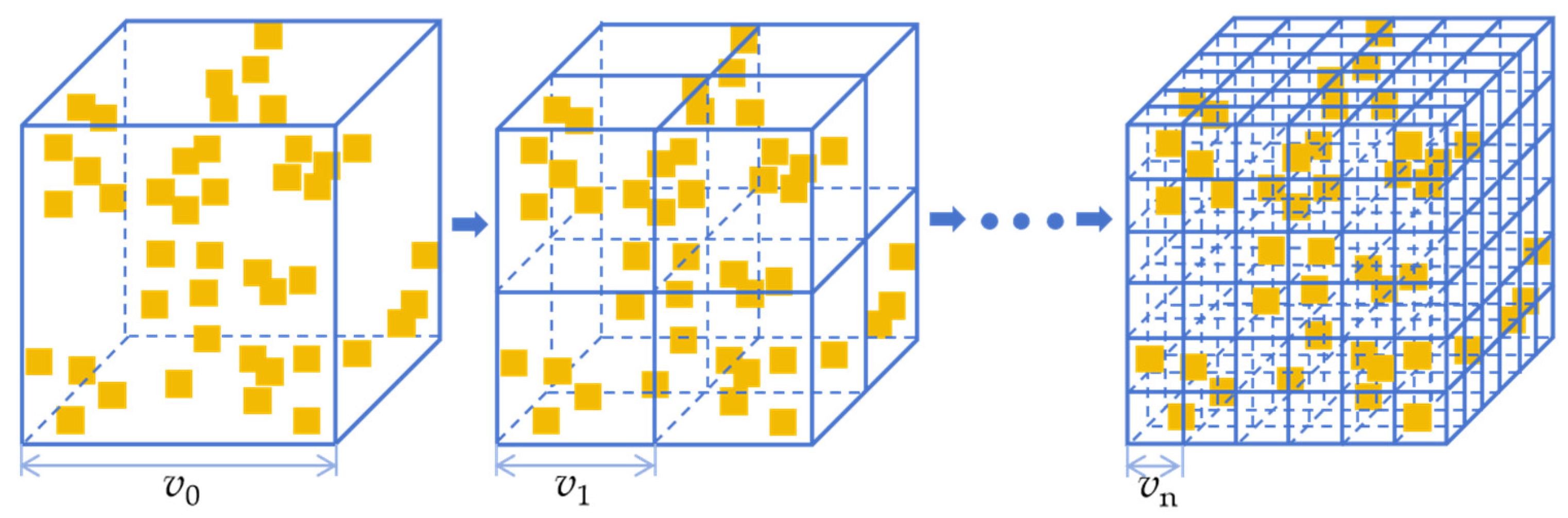
A multiscale voxel iteration method is implemented for point cloud downsampling. An optimized NDT algorithm is integrated with various filtering algorithms to register point clouds from both sources, and the effectiveness of different registration approaches is evaluated.

The rest of the paper is structured as follows. Section 2 introduces the framework for low-illumination accident scene reconstruction methods. In Section 3, the selection of investigative equipment is discussed. The method for point cloud processing is presented in Section 4. Section 5 demonstrates the feasibility of the registration method through preliminary experiments. Section 6 describes experiments under unobstructed and partially obstructed conditions, followed by an analysis of the results. Finally, Section 7 provides a summary of findings and future research directions.

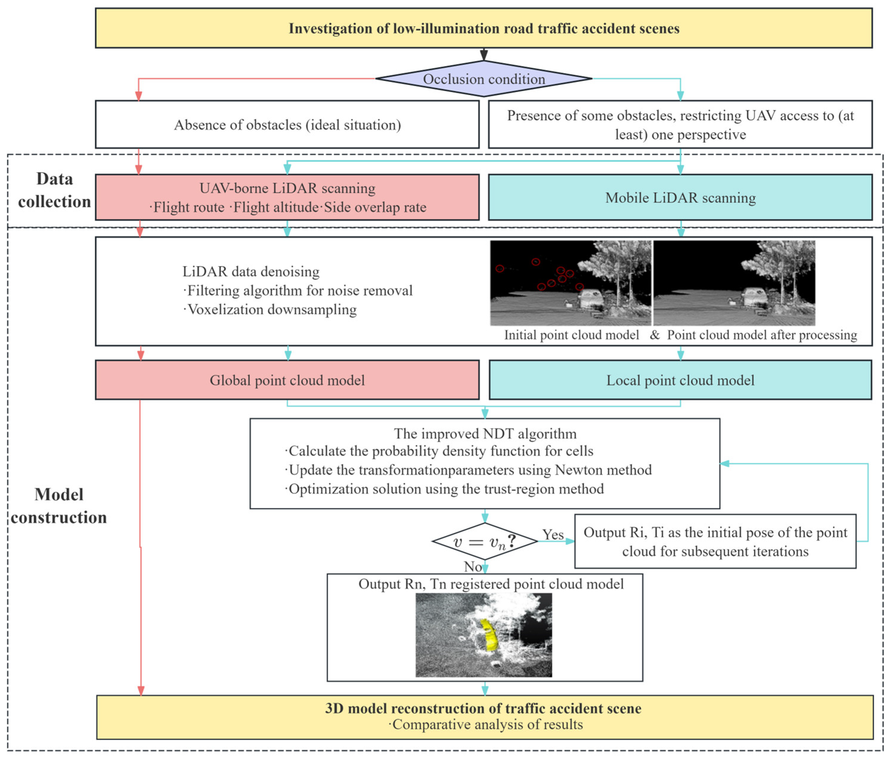
2. Methodological Framework for UAV-Assisted Accident Survey

The investigation method for low-illumination traffic accidents integrates various surveying tools to reconstruct a digital 3D model of the site. The traffic accident scenarios are classified into two categories based on the level of obstruction: (1) in the ideal case, with no obstacles, the UAV can autonomously follow a pre-planned flight path; (2) when partial obstructions limit the UAV’s access (from at least one perspective), the UAV can be manually controlled while a mobile laser scanner supplements point cloud data for the obstructed areas. The proposed methodology framework is illustrated in Figure 1.

First, the general accident situation is determined based on alarm information, then appropriate investigative strategies are selected according to different scenarios. As for the unobstructed scenarios, UAV flight paths are planned according to site-specific conditions. The airborne LiDAR system scans the accident scene, capturing wide-area information and the relative positions of key elements and surrounding objects, thereby directly generating a global point cloud model. In the scenes partially obstructed by traffic infrastructure or trees, a mobile LiDAR scanner supplements the airborne LiDAR by scanning areas that are obstructed or inaccessible to the airborne LiDAR, resulting in a local point cloud model that complements the missing sections of the airborne LiDAR scan. To complete the processing of the point clouds from two sources, a multiscale voxel iteration method for down sampling is combined with different filtering algorithms and the improved NDT algorithm for registration. The optimal methods and parameters are determined using the Autonomous Systems Lab (ASL) dataset [28], with the results applied to register the accident site’s global and local models. Finally, to assess the surveying accuracy of the proposed method, manual measurements and photogrammetric modeling are used to survey the same traffic accident. The results are compared and analyzed to evaluate the reconstruction accuracy and validate the practical utility of the proposed method.

3. Selection of Surveying Equipment

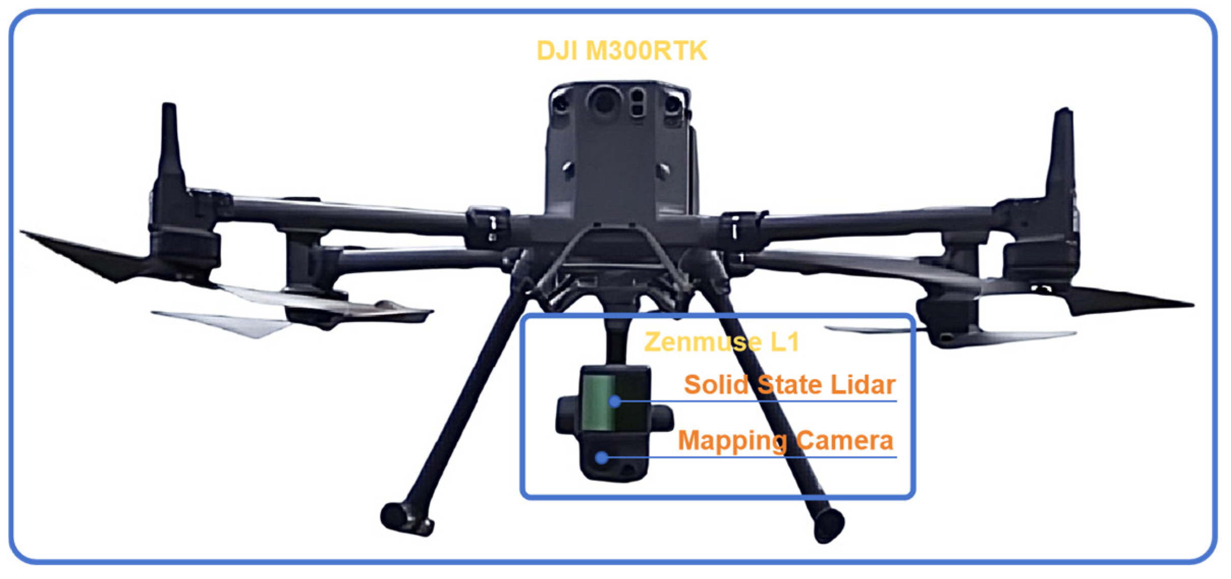
3.1. UAVs and Airborne LiDAR

UAVs are equipped with sensors such as an inertial navigation system, barometer, and global positioning system (GPS), enabling precise tracking of the UAV’s motion and attitude changes. In the previous study, Vida et al. [29] selected four UAVs, DJI Mavic Air2, DJI Air 2S, DJI Phantom, and DJI Inspire 1 v2.0, to test the feasibility of employing UAVs to effectively record the scene of a traffic accident in a short time. Additionally, the Johns Hopkins University [30] evaluated the operational systems for reconstructing traffic accident scenes using three UAVs, Leptron Quad Copter, Aeryon Sky Ranger, and DJI Inspire 1. These studies typically utilized UAVs equipped with cameras to capture images, followed by structure-from-motion (SFM) photogrammetry for model reconstruction. However, such methods fail to perform effectively under low-illumination conditions [31]. This study chooses the DJI M300 RTK UAV, integrated with the Zenmuse L1 airborne LiDAR system, as shown in Figure 2.

The DJI M300 RTK is equipped with stereo visual and infrared sensors, enabling six-way positioning and obstacle avoidance, and it can support up to three payloads simultaneously with a flight endurance of up to 55 min. The Zenmuse L1 integrates high-precision inertial navigation, a mapping camera, and a three-axis gimbal, allowing the system to capture its sensor coordinates, including longitude, latitude, and altitude during operations. Each mission can cover an area of up to 2 km², with vertical accuracy of 5 cm and planar accuracy of 10 cm. This system supports all-weather, high-efficiency, real-time 3D data acquisition and high-precision reconstruction of complex scenes.

During UAV operations, factors including flight management regulations, obstacles along the flight path, and adverse weather conditions must be carefully considered. Surveying tasks should be planned based on the specific conditions at the site. The following key elements must be considered to ensure operational safety.

1.

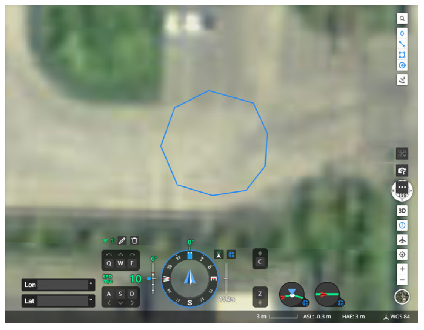
Flight Path: Common flight patterns include back-and-forth and circular modes. The flight path is selected based on the scale of the accident [32]. The back-and-forth mode is suitable for large-scale accident sites (e.g., multi-vehicle collisions on highways) extending over 50 m, allowing rapid coverage of a large area. The circular flight mode is ideal for smaller accident sites (e.g., single-vehicle collisions) or fall-type accidents (e.g., vehicles falling off a cliff), and the UAV flies in a circle trajectory with the center at the target area and the radius extending to the accident farthest point, ensuring comprehensive data collection from multiple viewpoints. Since the simulated traffic accident scene is small, and the aerial survey aims to acquire the relative positions and geometric information of the accident objects, thus, the circular flight path is specially selected.

2.

Flight Altitude: In non-restricted areas of general urban environments, the maximum allowable altitude for UAV flights is 120 m. To minimize interference from irrelevant surrounding environment data and maintain scanning accuracy, the UAV should fly as close to the accident site. However, real-world road environments often include obstacles such as streetlights, traffic signage, and trees, usually around 12 m high, necessitating adjustments to the flight altitude based on the specific obstacles at the accident site. Zulkifli et al. [20] recommended a drone flight height of 15 m for aerial survey, which can ensure the drone flight safety and avoid the environment obstacles, such as trees, traffic infrastructure, and so on. Therefore, this study selects a drone flight height of 15 m.

3.

Side Overlap Rate: Airborne LiDAR systems can collect high-density point cloud data from multiple perspectives, allowing for precise capture of the geometric features and three-dimensional information of accident sites. A scan overlap rate exceeding 50% is typical to ensure adequate data coverage. The point cloud data from different perspectives are integrated and processed using the side overlap rate and pose data, ultimately generating high-precision 3D models or point cloud datasets.

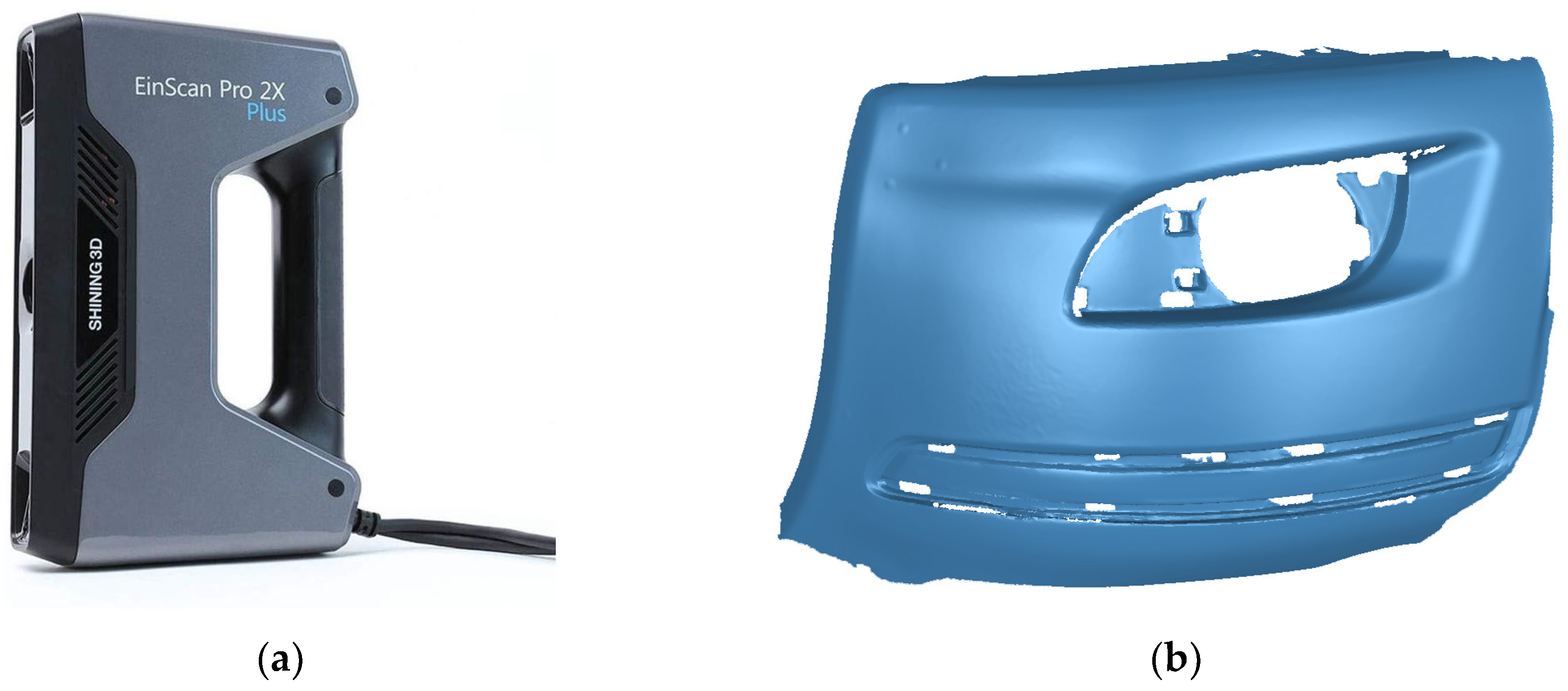
A high-precision inertial guidance system can help the UAV-borne LiDAR system to sense UAV flight motion and obtain real-time position and attitude data. However, inertial guidance systems exhibit time-dependent drift, leading to error accumulation over extended operation. Therefore, it is essential to conduct the calibration among different sensors. A color camera integrated into the UAV-borne LiDAR system can capture images with distinctive features. The feature point information of these images can be used to estimate the inverse position, thus facilitating the calibration of the inertial guidance system. Based on the position and attitude information obtained from the inertial guidance system at different scanning instances, high-precision stitching of point cloud data from multiple scans can be achieved to reconstruct the 3D point cloud model. In this study, to calibrate the inertial guidance system in the DJI Zenmuse L1 LiDAR, ground control points (GCPs) with known latitude and longitude coordinates are deployed on the accident scene ground. GCPs can be obtained using the Global Navigation Satellite System (GNSS) in the WGS84 coordinate system, which records the latitude, longitude, and altitude of ground reference points. To extract the camera images, GCPs must have distinct features, which are beneficial for determining the positional transformation relationship of different viewpoints.

Based on the feature point information of the two overlapped images, the sensor’s rotation and translation matrix between the two frames can be determined using epipolar geometric constraints. Thus, the sensor motion between the two frames is recovered. Through calibration computations, the rotation and translation matrices are obtained, as shown below.

$$R=\left[\begin{array}{ccc}0.99992& 0.01203& -0.00465\\ 0.01193& -0.99972& -0.02048\\ -0.00489& 0.02042& -0.99976\end{array}\right]$$

(1)

$$t=[35.08001, 16.94006, 46.43998]$$

(2)

The file containing the rotation and translation matrix data is then loaded into the LiDAR device to complete self-calibration.

3.2. Mobile LiDAR

Mobile LiDAR can rapidly generate high-precision 3D point cloud models of smaller objects, such as components, accurately reflecting the actual conditions of the measured objects, while it struggles to scan large objects or those without distinctive points. Therefore, mobile LiDAR is used to perform detailed modeling of occluded or collision-induced damage, filling in missing details and maximizing the retention of original accident site information for high-precision surveying.

Before scanning the accident site, a calibration board containing clear feature information (e.g., dimensions, distances, shapes) is used to calibrate the mobile laser radar. The point cloud accuracy is assessed by comparing the measured values of the calibration board with the scanned data. For objects lacking obvious features, artificial feature points may be applied to assist with scanning and point cloud stitching.

This study chooses the EinScan Pro 2X, as shown in Figure 3. Using the EXScan V3.7 software to calibrate the EinScan Pro 2X mobile laser scanner by calculating the error between the measured values of the calibration board and the true values, the scanning error can be obtained as 0.02 cm. This result confirms that the device is in optimal working condition and suitable for high-precision modeling. When scanning, the EinScan Pro 2X mobile scanner continuously transmits data to the EXScan V3.7 software, and the software automatically performs data stitching using reference markers or feature points. Additionally, it enables real-time visualization, helping to prevent scanning defects caused by operational errors or the loss of feature points. The automotive part scanning with this scanner is shown in Figure 3, from which the fine details of the automotive part are clearly visible. This demonstrates that this scanner can reconstruct occluded data effectively.

The technical specifications of the UAV-borne LiDAR and mobile LiDAR are provided in

Table 1. LiDAR Parameters.

Equipment Parameters	Zenmuse L1	EinScan Pro 2X
Scanning frequency	240,000 points/second	1,500,000 points/second
Scanning accuracy	30 mm (within 100 m)	0.1 mm (within 0.5 m)
Weight of equipment	0.93 kg	1.25 kg
Splice mode	overlapping splicing	feature splicing
Data output	output 3D model after post-processing	direct output 3D model
Operating temperature	−20–50 °C	0–40 °C
Supported data format	PNTS/LAS/PLY/PCD/S3MB	OBJ/STL/ASC/PLY/P3/3MF

.

4. Point Cloud Processing

LiDAR-acquired point cloud data typically contain a vast number of points, and processing these data directly consumes significant computational resources and time. Pre-processing techniques reduce the number of data points, thereby reducing computational complexity and storage requirements while enhancing processing efficiency and transmission speeds. Additionally, raw point cloud data often include noise and redundant information that significantly deviates from the actual surface of the target object. The removal of these extraneous points can enhance model accuracy and readability. Furthermore, it is necessary to integrate point cloud data from multiple sources into a common coordinate system to construct a complete model in practical applications.

When handling the point cloud data, it is essential to comply with relevant technical standards and specifications strictly. The appropriate processing methods, tools, and parameters are determined by the model’s accuracy requirements and the distribution of the data points. Moreover, it is crucial to avoid data loss or distortion to maintain data consistency and integrity during processing, ensuring that the result accurately reflects real-world conditions. Additionally, as point cloud data may contain sensitive information, particular attention must be paid to data security and privacy protection to prevent leakage or misuse.

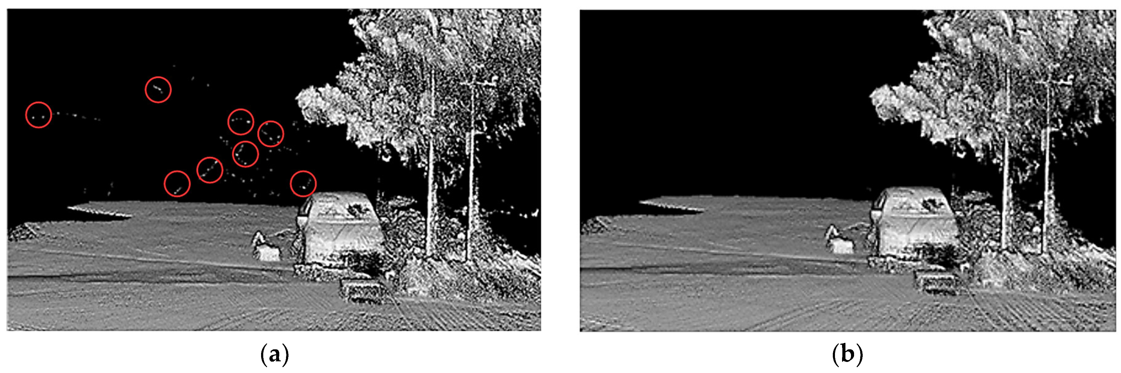
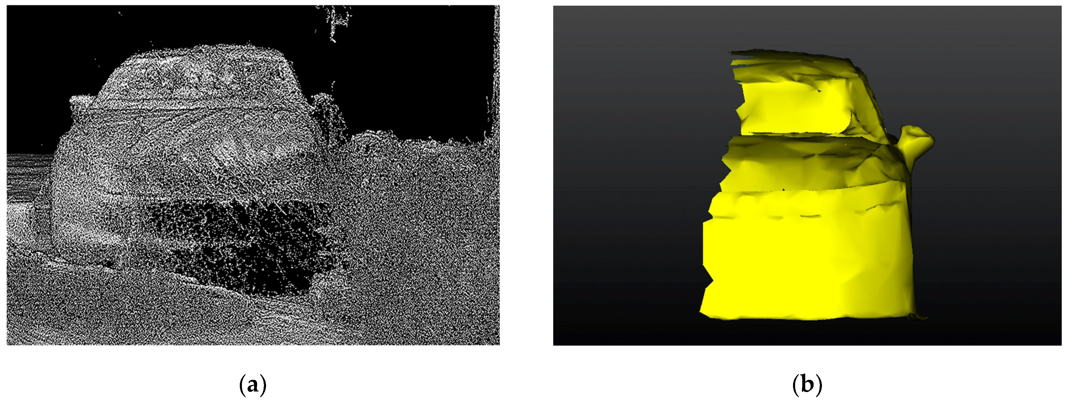
4.1. Denoising and Downsampling of Point Clouds

Before point cloud registration and surface reconstruction, pre-processing methods, such as filtering and voxelization downsampling, are employed to process the raw point cloud data. These methods reduce computational complexity while preserving the original geometric structure of the point cloud model.

Filtering algorithms commonly employed for noise removal include mean filtering, median filtering, and Gaussian filtering. These algorithms identify and eliminate noise points based on the statistical characteristics and distribution patterns. Mean filtering replaces the original value with the average of the surrounding points, offering good smoothing capabilities for normally distributed random noise; however, it may distort edges and result in the loss of important features. Median filtering, which substitutes the original value with the median of surrounding points, effectively removes impulse and salt-and-pepper noise while preserving edge details. However, it is computationally slower and less effective at eliminating mixed, similar noise. Gaussian filtering utilizes a weighted average to preserve the original data appearance but may lose critical point information at edges and corners. Thus, the choice of algorithm should be based on specific requirements.

Voxel-based downsampling divides the point cloud into spatial segments based on voxel size, generating a series of uniform voxel units. Voxel size plays a critical role in both registering accuracy and processing efficiency. A larger voxel size may fail to capture fine surface features and reduce registration accuracy. In contrast, smaller voxels generally provide more precise spatial information, enhancing registration accuracy. However, excessively small voxel size will increase process time and algorithm sensitivity to noise. Therefore, voxelization of the point cloud is carried out using voxels of progressively smaller sizes $(v_0,v_1,v_2,\dots ,v_n)$. Figure 4 illustrates the process of multiscale voxel-based downsampling of the point cloud. Then the centroid of each non-empty voxel is computed, and the centroid coordinates serve as an approximate representation of all points within the same voxel. In cases where a centroid cannot be directly identified, the point closest to the centroid is chosen as a substitute. This procedure efficiently achieves the point cloud downsampling.

4.2. Improved NDT Algorithm for Point Cloud Registration

Point cloud models from airborne LiDAR and mobile LiDAR scanning are registered by adjusting their relative positions through rotation and translation, without altering the structural characteristics of the models. This process achieves precise integration of the two datasets. Existing data processing algorithms often produce different results depending on the order of the input data. Therefore, algorithms that are suitable for the features of point cloud data should be employed. Usually, summing or taking the maximum value is adopted to obtain features independent of point order.

The iterative closest point (ICP) algorithm, which aligns and integrates point clouds by estimating the relative pose between them, is a widely used point cloud registration method. This method does not rely on point cloud segmentation or feature extraction [33]. However, the ICP algorithm only considers the distances between points, disregarding point cloud structural information, and it is sensitive to the initial values and unsuitable for matching global models with local models. Based on the large amounts of labeled data, deep learning methods have been used in the fields of fluid dynamics analysis [34], recognition of tensegrity structures [35], and point cloud registration [36,37]. However, the accident scenes under different weather and environment conditions are quite different, and the insufficient labeled data are the bottleneck to conduct the deep learning modeling.

To address these limitations, the normal distributions transform (NDT) algorithm has been used to register airborne LiDAR and handheld scanning models [38]. The NDT algorithm operates similarly to a grid-based approach, dividing the three-dimensional space into cells and assigning a normal distribution to each cell to model the probability of local measurement points. The primary objective of the process is to register scan $X$ to reference scan $Y$. The steps for the improved NDT algorithm are listed as follows.

Step 1: Conversion of point cloud to 3D normal distribution. The point cloud is partitioned into a three-dimensional grid, and the probability density function (PDF) of points within each grid cell is computed. We assume that $Y=\{y_1,y_2,\dots ,y_m\}$ represents the points in each cell, which is denoted as following a normal distribution. The mean vector $\overrightarrow{\mu }$ and the covariance matrix calculations $\mathrm{z}$ can be given by

$$\overrightarrow{\mu }={\displaystyle \frac{1}{m}}\sum _{k=1}^m\overrightarrow{y_k}$$

(3)

$$\mathrm{z}={\displaystyle \frac{1}{m-1}}{\sum }_{k=1}^m\left(\overrightarrow{y_k}-\overrightarrow{\mu }\right){\left(\overrightarrow{y_k}-\overrightarrow{\mu }\right)}^T$$

(4)

where $m$ represents the number of points in the current voxel, and $\overrightarrow{y_k}$ denotes the vector of the kth reference point within the voxel.

When the mean and covariance matrices are calculated, the PDF of the multivariate normal distribution can be expressed as follows:

$$f\left(\overrightarrow{x}\right)={\displaystyle \frac{1}{{\left(2\mathsf{\pi }\right)}^{\frac{3}{2}}\sqrt{\left|z\right|}}}{\mathrm{e}}^{-{\displaystyle \frac{(\overrightarrow{x}-\overrightarrow{\mu }{)}^T{\mathrm{z}}^{-1}(\overrightarrow{x}-\overrightarrow{\mu })}{2}}}$$

(5)

where $({\left(2\mathsf{\pi }\right)}^{{\displaystyle \frac{3}{2}}}\sqrt{\left|z\right|}{)}^{-1}$ is used to scale the function such that its integral equals 1, with the constant typically substituted in its place. The normal distribution represents the discrete points within each grid, with each PDF approximating the local surface. This approximation encapsulates information regarding the surface’s position, orientation, and smoothness in space.

Step 2: A voxelization method is employed to downsample the point cloud data, preserving key geometric features of the original dataset while reducing processing time. Voxelization of the point cloud is performed using a sequence of decreasing voxel sizes $(v_0,v_1,v_2,\dots ,v_n)$, with point cloud registration carried out progressively. The parameters from the previous registration are utilized as input for subsequent iterations, realizing a gradual alignment until the smallest voxel size $v_n$ is achieved.

The minimum voxel size is determined based on local geometric flatness [39]. By analyzing the covariance matrix of each voxel’s point set, eigenvalues are derived and arranged in descending order as ${\lambda }_0\ge {\lambda }_1\ge {\lambda }_2$. The geometric flatness of the corresponding voxel is then calculated as $f={\lambda }_2/({\lambda }_0+{\lambda }_1+{\lambda }_2)$. Given the flatness threshold $\mathrm{T}$ (here it is set to 0.005), voxels in the target point cloud with a flatness value satisfy the condition of $f\le \mathrm{T}$ are identified as exhibiting flat characteristics. The voxel flatness ratio of the point cloud is defined as the proportion of voxels exhibiting flat attributes to the total number of voxels in the target point cloud. The flatness ratio can be expressed as follows:

$$\mathrm{R}\mathrm{a}\mathrm{t}\mathrm{i}\mathrm{o}={\displaystyle \frac{\mathcal{N}\left\{{\mathrm{V}\mathrm{o}\mathrm{x}\mathrm{e}\mathrm{l}}_{f\le T}\right\}}{\mathcal{N}\left\{\mathrm{V}\mathrm{o}\mathrm{x}\mathrm{e}\mathrm{l}\right\}}}$$

(6)

where $\mathcal{N}\left\{·\right\}$ is the statistical function for determining the number of voxels meeting certain criteria. The minimum voxel size is determined when the voxel flatness ratio of the point cloud reaches its maximum, as expressed by the following equation:

$$v_n=v^{\ast }={\mathrm{a}\mathrm{r}\mathrm{g}\mathrm{m}\mathrm{a}\mathrm{x}}_v{\displaystyle \frac{\mathcal{N}\left\{{\mathrm{V}\mathrm{o}\mathrm{x}\mathrm{e}\mathrm{l}}_{f\le \mathcal{T}}\right\}}{\mathcal{N}\left\{\mathrm{V}\mathrm{o}\mathrm{x}\mathrm{e}\mathrm{l}\right\}}}$$

(7)

The initial voxel size, $v_0$, is set to the maximum, and each subsequent voxel is reduced by 20% of the previous voxel size until the minimum voxel size, $v_n$, is reached.

Step 3: After calculating the probability density function for each voxel, the optimal transformation needs to be identified. The LiDAR point cloud set is represented as $X=\{x_1,x_2,\dots ,x_{\mathrm{n}}\}$, with the transformation parameters denoted as $\overrightarrow{p}$. The spatial transformation function $T(\overrightarrow{p},\overrightarrow{x_k})$ describes the movement of point $\overrightarrow{x_k}$ using the transformation parameters $\overrightarrow{p}$. Combining the state density function computed earlier, the optimal transformation parameters $\overrightarrow{p}$ correspond to the transformation that maximizes the likelihood function. The likelihood function is expressed as follows:

$$likelihood:\theta ={\prod }_{k=1}^{n}f\left(T(\overrightarrow{p},\overrightarrow{x_k})\right)$$

(8)

According to the principle that maximum likelihood is equivalent to minimizing the negative log-likelihood, it follows that

$$-log\theta =-\sum _{k=1}^{n}logf\left(T\left(\overrightarrow{p},\overrightarrow{x_k}\right)\right)$$

(9)

In practical applications, the normal distribution function is susceptible to noise or outliers, which can cause the negative log-likelihood to grow unbounded at extreme values far from the mean. Therefore, a bias representing noise and outliers is introduced, resulting in an enhanced probability density function:

$$\overline{f}\left(\overrightarrow{x}\right)=c_1{\mathrm{e}}^{-{\displaystyle \frac{(\overrightarrow{x}-\overrightarrow{\mu }{)}^T{\mathrm{z}}^{-1}(\overrightarrow{x}-\overrightarrow{\mu })}{2}}}+c_2ϵ$$

(10)

where $ϵ$ denotes the noise level. This function limits the impact of noise. The parameters $c_1$ and $c_2$ represent the weights of the normal distribution and the bias, respectively. By ensuring that the probability mass of $\overline{f}\left(\overrightarrow{x}\right)$ within the unit cell is equal to 1. The following expression is obtained when substituting Equation (10) into Equation (9):

$$-log\theta =-{\sum }_{k=1}^{n}log{(c}_1{\mathrm{e}}^{-{\displaystyle \frac{(\overrightarrow{x_k}-\overrightarrow{{\mu }_k}{)}^T{z_k}^{-1}(\overrightarrow{x_k}-\overrightarrow{{\mu }_k})}{2}}}+c_2ϵ)$$

(11)

where ${\mu }_k$ and $z_k$ denote the mean and covariance of the $k\mathrm{t}\mathrm{h}$ voxel, respectively. To reduce the complexity of the optimization and obtain the first and second derivatives of the log-likelihood function, the negative log-likelihood function is approximated by a Gaussian function, as follows:

$$\left\{\begin{array}{c}{d}_1=-\log \left(c_1+c_2\right)-d_3\\ d_2=-2\log ((-\log (c_1{\mathrm{e}}^{-{\displaystyle \frac{1}{2}}}+c_2)-d_3)/d_1)\\ d_3=-\log \left(c_2\right)\end{array}\right.$$

(12)

where $d_1$, $d_2,$ and $d_3$ are fitting parameters determined during the Gaussian approximation of the log-likelihood function. The influence of each point in the current scan on the NDT evaluation function is given by

$$\tilde{f}({\overrightarrow{x}}_k)=-d_1{\mathrm{e}}^{-{\displaystyle \frac{d_2(\overrightarrow{x_k}-\overrightarrow{{\mu }_k}{)}^T{z_k}^{-1}(\overrightarrow{x_k}-\overrightarrow{{\mu }_k})}{2}}}$$

(13)

The final NDT evaluation function is expressed as

$$S\left(\overrightarrow{p}\right)=-{\sum }_{k=1}^n \tilde{f}\left(T(\overrightarrow{p},\overrightarrow{x_k})\right)$$

(14)

Step 4: To solve for the transformation parameters $\overrightarrow{p}$, Newton’s method is employed to solve the equation as follows:

$$\left\{\begin{array}{c}H\Delta \overrightarrow{p}={\displaystyle \frac{\partial S}{\partial \overrightarrow{p}}}\\ \mathsf{s}.\mathsf{t}.\overrightarrow{p}=\{T_x,T_y,T_z,R_x,R_y,R_z\}\end{array}\right.$$

(15)

Newton’s method iteratively solves the equation $H\Delta \overrightarrow{p}=-\overrightarrow{g}$, where $H$ and $\overrightarrow{g}$ represents the Hessian matrix and gradient vector of $S\left(\overrightarrow{p}\right)$, respectively. $\Delta \overrightarrow{p}$ denotes the increase in the transformation matrix during the present iteration, allowing the transformation to be updated in the next iteration as $\overrightarrow{p}\leftarrow \overrightarrow{p}+\Delta \overrightarrow{p}$.

However, the stability of Newton’s method is relatively poor when used in isolation, leading to errors in the results. Additionally, the optimization process in Newton’s method involves polynomial expansion to approximate the objective function. The bias introduced during this process causes the expanded polynomial to fit the information in the original function inadequately. Therefore, constraints must be added to determine whether the fitted function can approximate the objective function within an acceptable error margin [40]. The trust region method is combined with Newton’s method for optimizing the NDT algorithm to improve the registration accuracy and efficiency between two-point cloud models. The constraint of the trust region method can be expressed as

$$\begin{array}{c}\underset{\Delta x}{min } m(\Delta x)=p(x_k)+g_k^T\Delta x+{\displaystyle \frac{1}{2}}\Delta x^T{H}_k\Delta x\\ \mathsf{s}.\mathsf{t}.\parallel \Delta x\parallel \le {\Delta }_k\end{array}$$

(16)

where $m$ represents the model function at the $k\mathrm{t}\mathrm{h}$ iteration, $p\left(x_k\right)$ is the objective function value at the current point $x_k$, $g_k$ is the gradient vector of the objective function at $x_k$, and $H_k$ denotes the Hessian matrix of the objective function at $x_k$. The increment $\Delta x$ refers to the change in the transformation matrix during the current iteration, which allows the update in the next iteration as $x_{k+1}\leftarrow x_k+\Delta x$; ${\Delta }_k$ is the trust region radius.

To select an appropriate trust region radius, the gain coefficient ${\gamma }_k$ is computed as follows:

$${\gamma }_k={\displaystyle \frac{p\left(x_k\right)-p\left(x_{k+1}\right)}{m\left(0\right)-m(\Delta x)}}$$

(17)

where $p\left(x_k\right)-p\left(x_{k+1}\right)$ represents the actual decrease in the objective function value, while $m\left(0\right)-m\left(\Delta x\right)$ denotes the predicted decrease. When ${\gamma }_k$ is close to 1, it indicates a good fit, allowing for an increase in the trust region radius to accelerate the search for the optimal solution. Conversely, when ${\gamma }_k$ is close to 0, it suggests that the fit has a large deviation, necessitating the optimization of the fitting function and a reduction in the trust region radius. The trust region radius is initialized as ${\Delta }_0=0.1\mathrm{m}$ and dynamically adjusted based on the gain coefficient ${\gamma }_k$. Specifically, if ${\gamma }_k>0.75$, the trust region radius is expanded to ${\Delta }_{\mathrm{k}+1}=1.5{\Delta }_{\mathrm{k}}$ to accelerate convergence; if ${\gamma }_k<0.25$, the radius is reduced to ${\Delta }_{\mathrm{k}+1}=0.5{\Delta }_{\mathrm{k}}$ to ensure accuracy. The Newton iteration terminates when the norm of the gradient vector falls below 1 × 10⁻⁶ or the maximum iteration count (set to 50) is reached. For the Hessian matrix $H$, a Levenberg–Marquardt damping factor $\lambda =0.01$ is incorporated to address inconsistent cases, modifying the update equation to $(H+\lambda I)\Delta p=-g$, where I denotes the identity matrix. This hybrid approach balances the quadratic convergence of Newton’s method with the global robustness of trust-region constraints.

During each iteration, the trust region method is employed to robustly update the registration parameters of the point cloud model, thereby enhancing efficiency and reducing the number of iterations, all while maintaining accuracy.

5. Preliminary Experiment: Verification of the Registration Method

5.1. ASL Dataset

An experimental analysis of registration accuracy is conducted to determine the optimal initial value settings for downsampling. Simultaneously, the effectiveness of combining various filtering algorithms with the optimized NDT algorithm in constructing 3D models of accident scenes is evaluated. The ASL dataset is adopted to measure the computational time and error of the registration method in the splicing of the global model and the local model. The ASL dataset includes 8 sequences of 3D laser point clouds, with approximately 35 point clouds in each sequence. This dataset comprises structured, semi-structured, and unstructured components, covering a variety of scenes such as apartments, park pavilions, and forests. Since the traffic accident scenes may contain different structured elements, such as vehicles, road infrastructure, and unstructured elements (e.g., trees and shrubs). Therefore, the semi-structured pavilion dataset with mixed scenes is selected to align with the practical objectives of the study.

5.2. Point Cloud Registration Analysis

The experiments were conducted on a platform, with an i7−12900k processor, 32 GB of RAM, and the Ubuntu 18.04 operating system, utilizing PCL 1.8.1 for the registration procedures.

To assess the effectiveness of the improved NDT algorithm, this study conducts comparative experiments with the classic NDT algorithm. The evaluation metrics employed in this study comprised data processing time and relative pose error (RPE). RPE is a metric that quantifies the discrepancy in positional alterations between two sequential scans conducted at an identical temporal interval, considering both rotational and translational components. However, translation error is generally considered the primary metric for evaluating overall error. The estimated poses set $P_1,\dots ,P_n$, the true poses set $Q_1,\dots ,Q_n$, the subscript denotes time $\mathrm{t}$, and $∆$ indicates the time interval.

$$E_i=\left(Q_i^{-1}{Q}_{i+\Delta }{)}^{-1}\right(P_i^{-1}{P}_{i+\Delta })$$

(18)

With the total number $\mathrm{n}$ and the time interval $∆$ known, $m=n-\Delta$ RPE values can be calculated. The root mean squared error (RMSE) is then used to quantify the error statistically, resulting in an overall value:

$$\mathrm{R}\mathrm{M}\mathrm{S}\mathrm{E}\left(E_{1n},\Delta \right)=({\displaystyle \frac{1}{m}}{\sum }_{i=1}^m \parallel trans(E_i){\parallel }^2{)}^{{\displaystyle \frac{1}{2}}}$$

(19)

where $trans\left(E_i\right)$ represents the translational error.

The comparison of registration time and errors for the classic and improved NDT on the ASL dataset is shown in

Table 2. The comparison of registration time and errors on the ASL dataset with different voxel sizes.

Model	Voxel Size
	1	0.8	0.6	0.4	0.2	0.1
Classic NDT(Time/s|PRE)	6.15|0.67	6.71|0.58	7.44|0.61	9.13|0.55	12.87|0.45	15.86|0.43
Improved NDT(Time/s|PRE)	6.82|0.62	7.69|0.59	8.35|0.55	9.75|0.50	14.15|0.39	18.26|0.36

.

As shown in Table 2, the improved and classic NDT algorithms exhibit significant variations in terms of registration accuracy and processing time with voxel sizes ranging from 0.1 to 1.0. As the voxel size decreases, the processing time increases. However, the computational time of the improved NDT algorithm is higher than that of the classic NDT algorithm. This is because the improved NDT employs a multiscale voxel iteration strategy that helps the optimization process avoid local optima. It should be noted that the improved NDT algorithm achieves significantly higher registration accuracy than the classic NDT algorithm in different voxel resolutions. This confirms the effectiveness and feasibility of the improved NDT algorithm.

Based on the practical requirements for 3D reconstruction at accident sites, different registration methods are evaluated to identify the optimal registration approach and parameter settings. To determine the most suitable point cloud processing parameters, three voxel sizes: 0.1, 0.2, and 0.3, were tested for downsampling the point clouds. The mean, median, and Gaussian filtering algorithms were integrated with the NDT algorithm to register the point cloud models, and the optimal solution was obtained through comparative analysis.

The performance for different registration algorithms is summarized in

Table 3. Analysis of registration results.

Downsampling Parameters	Registration Algorithms	Processing Time/s	RPE
0.1	Gaussian filtering + improved NDT	20.38	0.32
0.1	mean filtering + improved NDT	20.62	0.36
0.1	median filtering + improved NDT	21.12	0.35
0.2	Gaussian filtering + improved NDT	15.54	0.34
0.2	mean filtering + improved NDT	15.83	0.37
0.2	median filtering + improved NDT	16.11	0.38
0.3	Gaussian filtering + improved NDT	10.21	0.45
0.3	mean filtering + improved NDT	10.74	0.48
0.3	median filtering + improved NDT	11.38	0.51

.

As demonstrated in Table 3, when the initial voxel size for point cloud downsampling is set to 0.1, the number of points remains substantial, leading to excessive processing time. Conversely, a voxel size of 0.3 reduces the processing time but causes a significant decrease in registration accuracy. When the voxel size is set to 0.2, the registration accuracy does not decrease significantly compared to when the voxel size is set to 0.1, while the processing time is noticeably reduced.

Furthermore, low-illumination aerial image data often contain sensor noise that is approximately Gaussian-distributed. To address this, Gaussian filtering is employed due to its weighted averaging mechanism, which effectively reduces noise while preserving smooth edges in accident scene reconstruction, such as vehicle contours and road markings. Mean filtering blurs sharp features, while median filtering may distort subtle geometric details under mixed noise conditions. In this context, Gaussian filtering provides a more balanced noise reduction. This can ensure the improved data fidelity, aligning with the accuracy required for traffic accident reconstruction.

Consequently, a voxel size of 0.2 is selected for point cloud downsampling in subsequent experiments. Following noise removal through the implementation of Gaussian filtering, the optimized NDT algorithm is utilized for point cloud registration.

6. Field Experiment and Its Analysis

A simulated traffic accident scene was implemented at Tianjin University of Technology and Education, China. To assess the effectiveness of the proposed method in low-illumination traffic accident scenarios, common urban obstacles, such as traffic signals, streetlights, vegetation, and trees, were included in the simulated collision scene. The low-illumination conditions were created at night with natural light sources such as moonlight and streetlights along the road. Given the relatively limited scope of the simulated accident scenes, the primary measurement is the geometric information of objects within the scene. During the airborne LiDAR scanning process, the UAVs followed circular flight paths at an altitude of 15 m, enabling the UAV’s proximity to the scene while avoiding obstacles to ensure flight safety. The UAV flight path was set as shown in Figure 5. The scan side overlap rate was 50% to ensure the collected point cloud data met the required surveying accuracy.

Operators could remotely control UAVs using dedicated controllers or high-performance computers (as shown in Figure 6), ensuring operational flexibility and precision while significantly expanding the operational range and enhancing safety. The system enabled real-time transmission of high-resolution UAV-captured images from accident scenes to remote interfaces, providing critical visual data for immediate situation assessment. This process substantially improving the rescue efficiency and incident management effectiveness.

To validate the proposed method, the constructed point cloud model was compared with traditional surveying methods and aerial photography modeling techniques. To obtain aerial photogrammetry modeling results, the UAV with a camera was used to capture image data of the traffic accident site from various altitudes and angles. Subsequently, high-precision pose data recorded during the UAV flight were utilized for image feature extraction and matching, leading to the construction of both sparse and dense point cloud models. Finally, a 3D aerial photogrammetry model of the accident site was generated through meshing and texturing processes.

The processing workflow was implemented in Agisoft Metasheape PhotoScan Professional v1.8.2 software, with the following SFM parameters: the number of key points is set to 100,000, the number of tie points is set to 40,000, and the dense cloud quality is set to high level. Simultaneously, advanced matching was enabled to improve feature point correspondence. The comparison between aerial photographic modelling and UAV-borne LiDAR modelling is shown in

Table 4. The comparison between aerial photographic modelling and UAV-borne LiDAR modelling.

Attribute	Aerial Photography Modeling	UAV-Borne LiDAR Modeling
Data acquisition	RGB images	Point cloud
Light condition	Sufficient	None
Imaging principle	Pinhole imaging	Laser reflection
Export result	3D model	Point cloud model
Color and texture	Exist	None
Resolution	High	Low
Noise	None	Exist
Cost	Cheap	Expensive

.

Based on the reconstructed 3D model, different objects were measured using the 3D model measurement tool MeshLab. The straight-line distance between two feature points on the same object represents the object’s dimensions. To ensure the reliability, each part was measured three times, and the average value was taken to enhance measurement accuracy. To evaluate measurement accuracy, tape-measured values were used as the baseline dimensions. The relative error (RE) and RMSE between the true and measured values of the objects in the accident scene were calculated to evaluate the error levels. RE measures the accuracy of individual measurements, while RMSE assesses the performance of the overall measurement process. In the RMSE calculation, data points with a RE greater than twice the standard deviation (SD), i.e., $\left|RE\right|>2\times SD$, are considered outliers and excluded from the analysis.

$$RE={\displaystyle \frac{L_{im}-L_{it}}{L_{it}}}\times 100\mathrm{\%}$$

(20)

$$RMSE=({\displaystyle \frac{1}{n}}{\sum }_{i=1}^n {RE}^2{)}^{{\displaystyle \frac{1}{2}}}$$

(21)

$$SD=\sqrt{{\displaystyle \frac{\sum _{i=1}^n ({RMSE}_i-\stackrel{¯¯¯¯¯¯¯¯¯¯¯¯}{RMSE}{)}^2}{n-1}}}$$

(22)

where n represents the total number of measured objects, $i$ represents the $i\mathrm{t}\mathrm{h}$ measured object, with the range of i defined as $0\le i\le n$; $L_{im}$ denotes the measured size of the object in the 3D model; and $L_{it}$ denotes the true size of the object obtained using a tape measure. The resulting values were used to validate the surveying accuracy of the method proposed in this study.

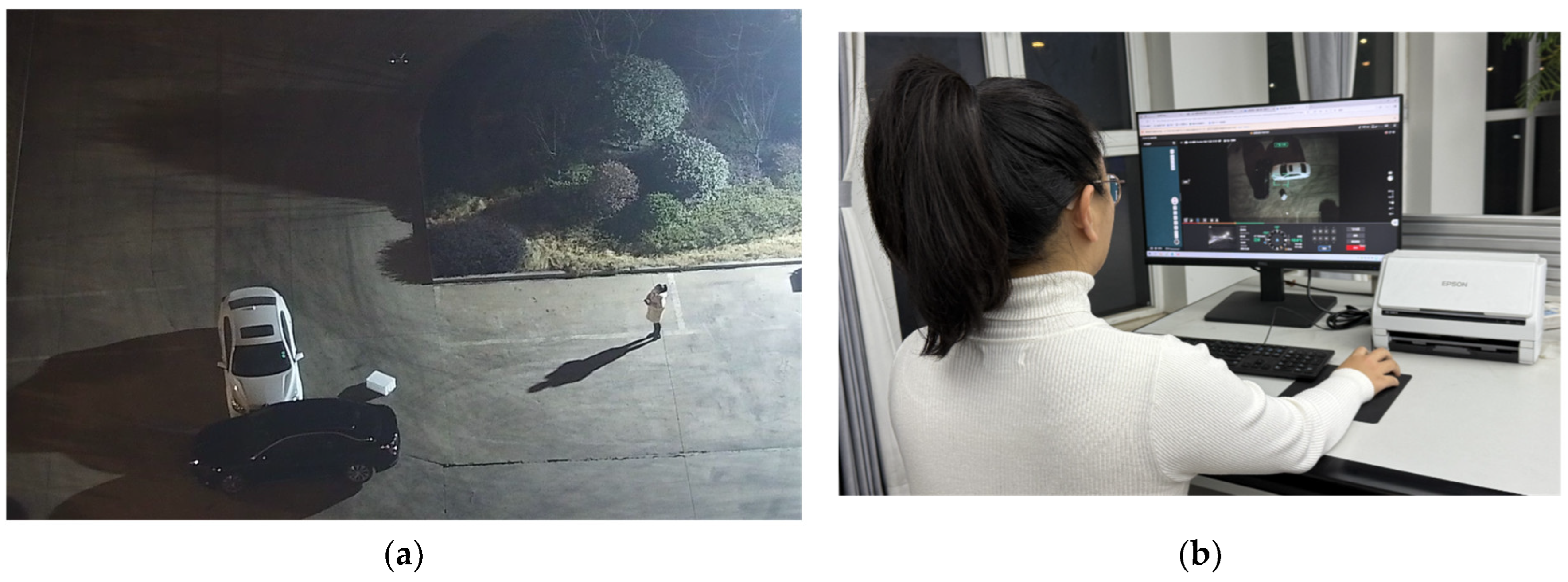
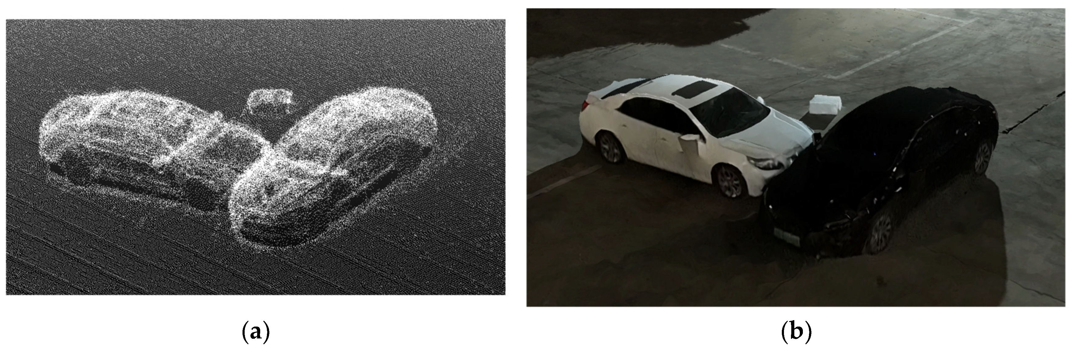
6.1. Scene 1: Traffic Accident in Low-Illumination Scene

The first scenario simulated a two-car collision in an open area under low-illumination conditions at night. The equipment box is representative of the scattered debris resulting from the collision. The experimental scene is shown in Figure 7.

In this experiment, there were no obstacles blocking the UAV’s flight. The flight path was planned using DJI Pilot, allowing the UAV to autonomously circle the accident scene. The data acquisition was conducted using airborne LiDAR and took 9 min 16 s, including UAV assembly, flight path planning, aerial scanning, and point cloud model processing.

The airborne LiDAR scanning conducted in this experiment resulted in a relatively complete point cloud model of the accident site. However, some noise points appeared near the surfaces of objects. To address this, downsampling and denoising were applied to the point cloud data, resulting in the final global point cloud model, shown in Figure 8. This model illustrates the vehicle positions and scattered debris in the simulated nighttime accident scene.

Additionally, aerial photography modeling took approximately 11 min 25s, which is longer than that of the proposed method in this study. The results captured by the UAV for this scene are presented in Figure 9.

Table 5. Modeling accuracy comparison with 11 measurement objects.

Measurement Number	Measurement Objects	Tape Measurement Length/m	Photography Modeling Length/m	UAV-Borne LiDAR Method Length/m	Photography Modeling RE/%	UAV-Borne LiDAR Method RE/%
1	Length of the white vehicle	4.88	4.83	4.92	−1.02	0.82
2	Width of the white vehicle	1.78	1.72	1.83	−3.37	2.81
3	Length of the black vehicle	4.93	4.77	4.99	−3.25	1.22
4	Width of the black vehicle	1.84	1.78	1.80	−3.26	−2.17
5	Right rear-view mirror of the white vehicle	0.21	0.20	0.23	−4.76	9.52
6	Right door handle of the white vehicle	0.26	0.25	0.27	−3.85	3.85
7	Right rear-view mirror of the black vehicle	0.22	0.25	0.24	13.64	9.09
8	Right door handle of the black vehicle	0.28	0.26	0.30	−7.14	7.14
9	Wheel diameter	0.65	0.62	0.66	−4.62	1.54
10	Length of box	0.75	0.80	0.79	6.67	5.33
11	Width of box	0.55	0.52	0.59	−5.45	7.27

presents a comparison of the two modeling approaches, while Figure 10 illustrates their results through visual representations.

According to Table 5, a longitudinal comparison indicates that airborne LiDAR modeling achieves higher accuracy when measuring larger objects. However, significant relative errors are observed when measuring smaller objects such as mirrors and equipment boxes. A horizontal comparison reveals that under low-illumination conditions, the accuracy of aerial photography modeling is noticeably inferior to that of UAV-borne LiDAR modeling, especially for darker and smaller objects. Based on the RMSE formula in Section 6, the outlier “Right rear-view mirror of the black vehicle” was excluded when calculating the RMSE for aerial photography modeling, resulting in an RMSE value of 0.0466 m. For the UAV-borne LiDAR method, the outliers “Right rear-view mirror of the white vehicle” and Right rear-view mirror of the black vehicle were excluded, yielding an RMSE value of 0.0427 m. Therefore, in low-illumination and unobstructed traffic accident scenarios, UAV-borne LiDAR modeling has smaller errors than aerial photography modeling.

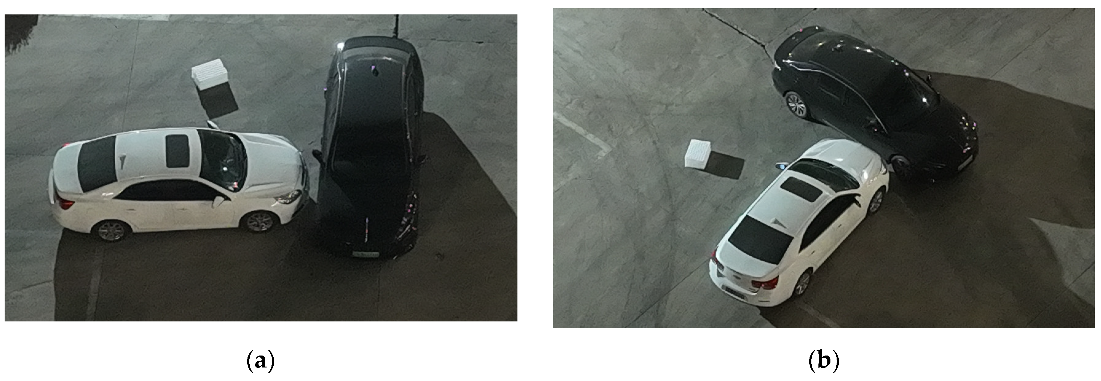
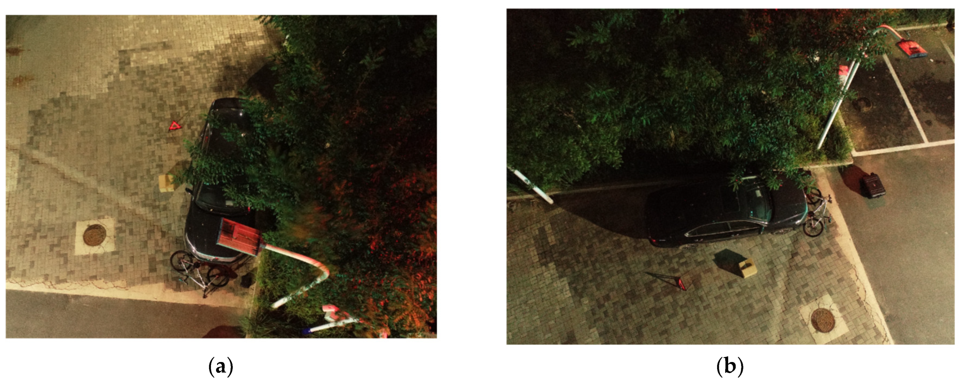
6.2. Scene 2: Traffic Accidents with Occlusion at Night

The second scenario simulates a bicycle-car collision in an area with partial occlusion under dim lighting conditions at night. This scene has common road infrastructure, such as utility poles, streetlights, and trees. The experimental scene is shown in Figure 11.

During the flight, it was observed that the UAV failed to directly capture the accident scene from certain angles due to the tree obstruction. Therefore, the flight path was manually adjusted to maximize the acquisition of on-site information while avoiding potential collisions with obstacles to ensure operational safety.

Additionally, the EinScan Pro 2X mobile laser scanner was used to scan the occluded sections of the accident scene and critical debris. Based on the registration analysis in Section 5.2, the initial voxel size was set to 0.2, and the global point cloud model underwent denoising and downsampling. As shown in Figure 12, the UAV inspection was affected by obstructions such as trees, which hindered direct and accurate observation of occluded objects from certain angles. As a result, point cloud data in the front collision area of the vehicle were partially missing.

The local point cloud model of the vehicle, acquired using the mobile laser scanner, was integrated with the global point cloud model to supplement missing data. Based on the experimental findings, Gaussian filtering and optimized NDT algorithms were applied to complete the registration process, resulting in a comprehensive point cloud model of the accident scene.

The registration results are shown in Figure 13. The total data collection time using the airborne LiDAR system and mobile laser scanner in this experiment was 13 min 43 s, including UAV assembly, flight path adjustment, flight scanning, handheld scanner scanning, point cloud registration, and model reconstruction. The aerial photography modeling took approximately 15 min 28 s. The results indicate that in both experiments, aerial photography modeling required more time than the method proposed in this study. The mean reason is that the aerial photogrammetry method requires processing a large volume of image data during 3D reconstruction. This process involves recovering the three-dimensional information from images, making it more time-consuming.

The results captured by the UAV for this scene are presented in Figure 14.

Table 6. Modeling accuracy comparison with 12 measurement objects.

Measurement Number	Measurement Objects	Tape Measurement Length/m	Photography Modeling Length/m	UAV-Borne LiDAR Method Length/m	Photography Modeling RE/%	UAV-Borne LiDAR Method RE/%
1	Wheel diameter	0.65	0.61	0.67	−6.15	3.08
2	Length of the vehicle	4.93	4.81	4.99	−2.43	1.22
3	Width of the vehicle	1.84	1.77	1.79	−3.80	−2.72
4	Right rearview mirror	0.22	—	0.22	—	0.00
5	Right door handle	0.28	—	0.28	—	0.00
6	Length of box	0.75	0.81	0.80	8.00	6.67
7	Width of box	0.55	0.52	0.58	−5.45	5.45
8	Bicycle length	1.58	1.63	1.62	3.16	2.53
9	Bicycle wheel	0.56	0.58	0.60	3.57	7.14
10	Length of carton	0.42	0.46	0.45	9.52	7.14
11	Width of carton	0.42	0.45	0.44	7.14	4.76
12	Tripod length	0.44	0.46	0.48	4.55	9.09

presents a comparison of the two modeling approaches, while Figure 15 illustrates their results through visual representations.

As shown in Table 6, regarding the measurements of the right rearview mirror and right door handle, the mobile laser scanning method provides high-precision modeling, accurately representing the actual dimensions of the objects with negligible measurement error. In contrast, aerial photography or standalone airborne LiDAR scanning results in missing data due to obstructions, leading to reduced model accuracy. The boxes scattered around the scene after the collision are unobstructed, and their measurement via airborne LiDAR is generally more accurate than aerial photography. Based on the RMSE formula in Section 6, the outlier “Tripod length” was excluded when calculating the RMSE for the proposed method, resulting in an RMSE value of 0.0451 m, while the RMSE for aerial photography modeling is 0.0581 m. Compared to results from low-illumination and unobstructed scenarios in Section 6.1, it is evident that the accuracy of aerial photography modeling is significantly impacted by occlusions, leading to increased errors. In contrast, the accuracy of the proposed method remains relatively stable.

These results demonstrate that the ground–air accident investigation method proposed in this study offers broader applicability and higher precision than other methods. It effectively captures occluded sections of the accident scene and is unaffected by lighting conditions. This method is particularly suited for traffic accident investigations in low-illumination environments, enabling the rapid reconstruction of high-precision 3D point cloud models, which will support the accurate analysis of accident causes.

7. Conclusions and Discussions

This study presents a digital method for low-illumination traffic accident investigation aimed at constructing 3D point cloud models of accident scenes. The conclusions are drawn as follows.

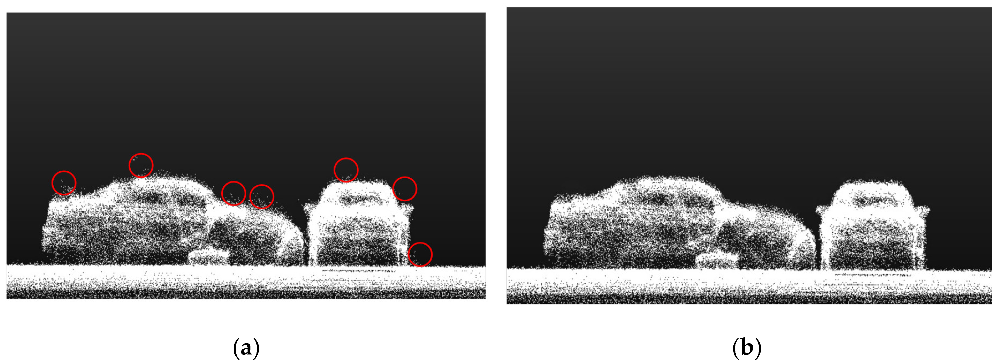
• The integration of airborne LiDAR and mobile laser scanning technologies is feasible and effective for traffic accident investigations. Airborne LiDAR rapidly generates a global point cloud model of the accident scene, unaffected by lighting conditions, while mobile scanners complement occluded regions. This method effectively addresses the issue of information loss caused by environmental factors, ensuring the integrity of accident scene data. Additionally, it facilitates the rapid completion of accident investigations, thereby reducing traffic congestion and preventing secondary accidents.
• A balanced trade-off between processing speed and accuracy was achieved when the voxel size was set to 0.2 and multiscale iterative downsampling was applied to the point cloud model. Compared to the mean and median filtering, Gaussian filtering and the optimized NDT algorithm have higher accuracy in 3D model reconstruction.
• Field experiments demonstrate that the proposed method outperforms the alternatives in traffic accident investigations under low illumination, generating high-precision, centimeter-level 3D models.

However, the proposed method still has certain limitations. Several aspects of using UAV-assisted accident scene reconstruction needs to be further explored as follows.

1.

Flight regulation and privacy protection. When utilizing UAVs for data collection, it is crucial to comply with the relevant laws, regulations, and privacy policies to ensure the legality and safety of the investigation. Operations in populated areas or restricted airspace must strictly adhere to airspace management regulations to avoid privacy infringements and public alarm. Additionally, UAV regulations differ across countries and regions, encompassing restrictions on flight altitude, designated areas, and operational time, which may influence the efficiency and effectiveness of UAV-based investigations. Furthermore, safeguarding personal privacy must remain a top priority. The stringent management of data storage and processing is crucial to ensuring data security, thereby increasing stakeholder acceptance of this technology.

2.

Environmental factors and weather. Extreme weather conditions, such as strong winds, heavy rain, lightning, or dense fog, will disrupt UAV operations and reduce the effective range of LiDAR sensing. Wet road surfaces and reflective objects may lead to erroneous laser returns and severely impact the UAV stability and data quality. In complex urban environments with dense buildings or structures, UAV flight and positioning may be constrained, thereby affecting the effectiveness of investigations. Additionally, electromagnetic interference from the accident site may disrupt UAV remote control and navigation systems, increasing operational complexity and risk. These challenges can be mitigated through a combination of hardware advancements and algorithmic enhancements. Developing waterproof UAVs will enable the operation in rainy and snowy weather. Designing UAVs with enhanced control mechanisms will improve the UAV flight stability in strong winds. Additionally, integrating multi-wavelength LiDAR sensors, refining signal processing algorithms, and employing AI-based noise filtering techniques can enhance data reliability under adverse weather conditions. Furthermore, fusing LiDAR data with inertial measurement unit (IMU) and GNSS information can improve positioning accuracy in GPS-denied environments, ensuring stable and high-quality data acquisition.

3.

Multi-source data fusion. The proposed method requires multi-source point cloud data processing. Traffic accident scenes are always complex and dynamic, and high-density point cloud data can lead to processing delays. Therefore, it is essential to explore modern data processing methods in the future. While deep learning techniques hold great promise for enhancing registration accuracy and automation, it still faces great challenges without large-scale labeled datasets of diverse accident scenarios. Future research could focus on developing domain adaptation strategies, self-supervised learning approaches, and robust feature extraction methods to improve the adaptability and efficiency of deep-learning-based registration techniques. By addressing these issues, it will be possible to achieve faster, more accurate, and more reliable 3D reconstruction of accident scenes under various environmental and operational constraints.

4.

Cost–efficiency balance. This approach provides substantial societal benefits by enabling rapid traffic accident investigations and reducing traffic congestion. Furthermore, it accurately preserves the accident scene in a 3D model, facilitating subsequent examinations. However, considering the costs of equipment acquisition, labor, and maintenance, the cost per investigation is approximately 400–500 RMB, indicating that the current method remains relatively costly. Further reduction in UAV hardware and software costs is crucial to enhance its practical applicability.

5.

Enhanced texture preservation. Photogrammetry can better represent textures, which is important for analyzing traffic accidents. However, in low-illumination traffic accident environments, the insufficient light received by the camera degrades the image quality, resulting in blurred surface textures and low measurement accuracy. To address this issue, the aerial RGB images can be used to color the LiDAR point cloud model, and this hybrid approach can ensure the geometric fidelity and visual texture.

References

1. Tang, J.; Huang, Y.; Liu, D.; Xiong, L.; Bu, R. Research on Traffic Accident Severity Level Prediction Model Based on Improved Machine Learning. Systems 2025, 13, 31. [Google Scholar] [CrossRef]
2. Tucci, J.; Dougherty, J.; Lavin, P.; Staes, L.; Safety, K.J. Effective Practices in Bus Transit Accident Investigations; United States, Department of Transportation, Federal Transit Administration: Washington, DC, USA, 2021; pp. 13–14. [Google Scholar]
3. Kamnik, R.; Perc, M.N.; Topolšek, D. Using the scanners and drone for comparison of point cloud accuracy at traffic accident analysis. Accid. Anal. Prev. 2020, 135, 105391. [Google Scholar] [CrossRef]
4. Garnaik, M.M.; Giri, J.P.; Panda, A. Impact of highway design on traffic safety: How geometric elements affect accident risk. Ecocycles 2023, 9, 83–92. [Google Scholar] [CrossRef]
5. Pagounis, V.; Tsakiri, M.; Palaskas, S.; Biza, B.; Zaloumi, E. 3D laser scanning for road safety and accident reconstruction. In Proceedings of the XXIIIth international FIG congress, Munich, Germany, 8–13 October 2006. [Google Scholar]
6. Buck, U.; Buße, K.; Campana, L.; Gummel, F.; Schyma, C.; Jackowski, C. What Happened Before the Run Over? Morphometric 3D Reconstruction. Forensic Sci. Int. 2020, 306, 110059. [Google Scholar] [CrossRef]
7. Calders, K.; Adams, J.; Armston, J.; Bartholomeus, H.; Bauwens, S.; Bentley, L.P.; Chave, J.; Danson, F.M.; Demol, M.; Disney, M.; et al. Terrestrial laser scanning in forest ecology: Expanding the horizon. Remote Sens. Environ. 2020, 251, 112102. [Google Scholar] [CrossRef]
8. Khodjaev, S.; Kuhn, L.; Bobojonov, I.; Glauben, T. Combining multiple UAV-Based indicators for wheat yield estimation, a case study from Germany. Eur. J. Remote Sens. 2024, 57, 2294121. [Google Scholar] [CrossRef]
9. Pensado, E.A.; López, F.V.; Jorge, H.G.; Pinto, A.M. UAV Shore-to-Ship Parcel Delivery: Gust-Aware Trajectory Planning. IEEE Trans. Aerosp. Electron. Syst. 2024, 60, 6213–6233. [Google Scholar] [CrossRef]
10. Wang, W.; Xue, C.; Zhao, J.; Yuan, C.; Tang, J. Machine learning-based field geological mapping: A new exploration of geological survey data acquisition strategy. Ore Geol. Rev. 2024, 166, 105959. [Google Scholar] [CrossRef]
11. Kong, X.; Ni, C.; Duan, G.; Shen, G.; Yang, Y.; Das, S.K. Energy Consumption Optimization of UAV-Assisted Traffic Monitoring Scheme with Tiny Reinforcement Learning. IEEE Internet Things J. 2024, 11, 21135–21145. [Google Scholar] [CrossRef]
12. Silva-Fragoso, A.; Norini, G.; Nappi, R.; Groppelli, G.; Michetti, A.M. Improving the Accuracy of Digital Terrain Models Using Drone-Based LiDAR for the Morpho-Structural Analysis of Active Calderas: The Case of Ischia Island, Italy. Remote Sens. 2024, 16, 1899. [Google Scholar] [CrossRef]
13. Neuville, R.; Bates, J.S.; Jonard, F. Estimating Forest Structure from UAV-Mounted LiDAR Point Cloud Using Machine Learning. Remote Sens. 2021, 13, 352. [Google Scholar] [CrossRef]
14. Zhang, Y.; Dou, X.; Zhao, H.; Xue, Y.; Liang, J. Safety Risk Assessment of Low-Volume Road Segments on the Tibetan Plateau Using UAV LiDAR Data. Sustainability 2023, 15, 11443. [Google Scholar] [CrossRef]
15. Cherif, B.; Ghazzai, H.; Alsharoa, A. LiDAR from the Sky: UAV Integration and Fusion Techniques for Advanced Traffic Monitoring. IEEE Syst. J. 2024, 18, 1639–1650. [Google Scholar] [CrossRef]
16. Wang, F.-H.; Li, L.-Y.; Liu, Y.-T.; Tian, S.; Wei, L. Road Traffic Accident Scene Detection and Mapping System Based on Aerial Photography. Int. J. Crashworthiness 2020, 26, 537–548. [Google Scholar]
17. Chen, Q.; Li, D.; Huang, B. SUAV image mosaic based on rectification for use in traffic accident scene diagramming. In Proceedings of the 2020 IEEE 3rd International Conference of Safe Production and Informatization (IICSPI), Chongqing, China, 28–30 November 2020. [Google Scholar]
18. Chen, Y.; Zhang, Q.; Yu, F. Transforming traffic accident investigations: A virtual-real-fusion framework for intelligent 3D traffic accident reconstruction. Complex Intell. Syst. 2025, 11, 76. [Google Scholar] [CrossRef]
19. Norahim, M.N.I.; Tahar, K.N.; Maharjan, G.R.; Matos, J.C. Reconstructing 3D model of accident scene using drone image processing. Int. J. Electr. Comput. Eng. 2023, 13, 4087–4099. [Google Scholar] [CrossRef]
20. Zulkifli, M.H.; Tahar, K.N. The Influence of UAV Altitudes and Flight Techniques in 3D Reconstruction Mapping. Drones 2023, 7, 227. [Google Scholar] [CrossRef]
21. Amin, M.; Abdullah, S.; Abdul Mukti, S.N.; Mohd Zaidi, M.H.A.; Tahar, K.N. Reconstruction of 3D accident scene from multirotor UAV platform. Int. Arch. Photogramm. Remote Sens. Spat. Inf. Sci. 2020, 43, 451–458. [Google Scholar] [CrossRef]
22. Pádua, L.; Sousa, J.; Vanko, J.; Hruška, J.; Adão, T.; Peres, E.; Sousa, J.J. Digital reconstitution of road traffic accidents: A flexible methodology relying on UAV surveying and complementary strategies to support multiple scenarios. Int. J. Environ. Res. Public Health 2020, 17, 1868. [Google Scholar] [CrossRef]
23. Pérez, J.A.; Gonçalves, G.R.; Barragan, J.R.; Ortega, P.F.; Palomo, A.A. Low-cost tools for virtual reconstruction of traffic accident scenarios. Heliyon 2024, 10, 1–26. [Google Scholar]
24. Nteziyaremye, P.; Sinclair, M. Investigating the effect of ambient light conditions on road traffic crashes: The case of Cape Town, South Africa. Light. Res. Technol. 2024, 56, 443–468. [Google Scholar] [CrossRef]
25. Liang, S.; Chen, P.; Wu, S.; Cao, H. Complementary Fusion of Camera and LiDAR for Cooperative Object Detection and Localization in Low-Contrast Environments at Night Outdoors. IEEE Trans. Consum. Electron. 2024, 70, 6392–6403. [Google Scholar] [CrossRef]
26. Li, Y.; Yu, A.W.; Meng, T.; Caine, B.; Ngiam, J.; Peng, D.; Shen, J.; Lu, Y.; Zhou, D.; Le, Q.V.; et al. Deep fusion: LiDAR-Camera Deep Fusion for Multi-Modal 3D Object Detection. In Proceedings of the IEEE/CVF Conference on Computer Vision and Pattern Recognition, New Orleans, LA, USA, 18–24 June 2022. [Google Scholar]
27. Hussain, A.; Mehdi, S.R. A Comprehensive Review: 3D Object Detection Based on Visible Light Camera, Infrared Camera, and Lidar in Dark Scene. Infrared Camera Lidar Dark Scene 2024, 2, 27. [Google Scholar]
28. Pomerleau, F.; Liu, M.; Colas, F.; Siegwart, R. Challenging data sets for point cloud registration algorithms. Int. J. Robot. Res. 2012, 31, 1705–1711. [Google Scholar] [CrossRef]
29. Vida, G.; Melegh, G.; Süveges, Á.; Wenszky, N.; Török, Á. Analysis of UAV Flight Patterns for Road Accident Site Investigation. Vehicles 2023, 5, 1707–1726. [Google Scholar] [CrossRef]
30. The Johns Hopkins University. Operational Evaluation of Unmanned Aircraft Systems for Crash Scene Reconstruction, 1st ed.; Applied Physics Laboratory: Laurel, MD, USA, 2018; pp. 27–29. [Google Scholar]
31. Liu, S.; Wei, Y.; Wen, Z.; Guo, X.; Tu, Z.; Li, Y. Towards robust image matching in low-luminance environments: Self-supervised keypoint detection and descriptor-free cross-fusion matching. Pattern Recognit. 2024, 153, 110572. [Google Scholar] [CrossRef]
32. Zheng, J.; Yang, Q.; Liu, J.; Li, L.; Chai, Y.; Xu, P. Research on Road Traffic Accident Scene Investigation Technology Based on 3D Real Scene Reconstruction. In Proceedings of the 2023 3rd Asia Conference on Information Engineering (ACIE), Chongqing, China, 22 August 2023. [Google Scholar]
33. Besl, P.J.; McKay, N.D. Method for registration of 3-D shapes. In Sensor Fusion IV: Control Paradigms and Data Structures; Society of Photo-Optical Instrumentation Engineers: Boston, MA, USA, 1992. [Google Scholar]
34. Peng, Y.; Yang, X.; Li, D.; Ma, Z.; Liu, Z.; Bai, X.; Mao, Z. Predicting Flow Status of a Flexible Rectifier Using Cognitive Computing. Expert Syst. Appl. 2025, 264, 125878. [Google Scholar] [CrossRef]
35. Mao, Z.; Kobayashi, R.; Nabae, H.; Suzumori, K. Multimodal Strain Sensing System for Shape Recognition of Tensegrity Structures by Combining Traditional Regression and Deep Learning Approaches. IEEE Robot. Autom. Lett. 2024, 9, 10050–10056. [Google Scholar] [CrossRef]
36. Huang, X.; Mei, G.; Zhang, J.; Abbas, R. A Comprehensive Survey on Point Cloud Registration. arXiv 2021, arXiv:2103.02690. [Google Scholar]
37. Shen, Z.; Feydy, J.; Liu, P.; Curiale, A.H.; San Jose Estepar, R.; Niethammer, M. Accurate Point Cloud Registration with Robust Optimal Transport. Adv. Neural Inf. Process. Syst. 2021, 34, 5373–5389. [Google Scholar]
38. Biber, P.; Straßer, W. The normal distributions transform: A new approach to laser scan matching. In Proceedings of the 2003 IEEE/RSJ International Conference on Intelligent Robots and Systems (IROS 2003), Las Vegas, NV, USA, 27–31 October 2003. [Google Scholar]
39. Shen, Y.; Zhang, B.; Wang, J.; Zhang, Y.; Wu, Y.; Chen, Y.; Chen, D. MI-NDT: Multiscale Iterative Normal Distribution Transform for Registering Large-scale Outdoor Scans. IEEE Trans. Geosci. Remote Sens. 2024, 62, 5705513. [Google Scholar] [CrossRef]
40. Mohammadi, A.; Custódio, A.L. A trust-region approach for computing Pareto fronts in multiobjective optimization. Comput. Optim. Appl. 2024, 87, 149–179. [Google Scholar] [CrossRef]
Figure 1. Methodological framework for accident survey.
Wevj 16 00171 g001
Figure 2. DJI M300RTK loaded with Zenmuse L1.
Wevj 16 00171 g002
Figure 3. Mobile scanning equipment and scan results. (a) EinScan Pro 2X mobile laser scanner; (b) Results of automotive part scanning with the EinScan Pro 2X.
Wevj 16 00171 g003
Figure 4. The process of multiscale voxel-based downsampling of the point cloud.
Wevj 16 00171 g004
Figure 5. The UAV flight path.
Wevj 16 00171 g005
Figure 6. The ways for UAV operation. (a) Remote controller; (b) High-performance computer.
Wevj 16 00171 g006
Figure 7. Accident scene at night. (a) Front view; (b) Side view.
Wevj 16 00171 g007
Figure 8. Scene 1 point cloud model preprocessing. (a) initial point cloud model; (b) processed point cloud model.
Wevj 16 00171 g008
Figure 9. Comparison of modeling results. (a) Comparison of modeling results; (b) Aerial photography modeling.
Wevj 16 00171 g009
Figure 10. The RE of the measurement results for different methods in scene 1. (a) Photography modeling; (b) UAV-borne LiDAR method.
Wevj 16 00171 g010
Figure 11. Accident scene with occlusion at night. (a) Front view; (b) Side view.
Wevj 16 00171 g011
Figure 12. Scene 2 point cloud model preprocessing. (a) initial point cloud model; (b) processed point cloud model.
Wevj 16 00171 g012
Figure 13. Point cloud model visualization. (a) UAV-borne LiDAR modeling of car at front view; (b) mobile LiDAR scanning modeling of car at front view; (c,d) model registration results.
Wevj 16 00171 g013aWevj 16 00171 g013b
Figure 14. Aerial photography modeling.
Wevj 16 00171 g014
Figure 15. The RE of the measurement results for different methods in scene 2. (a) Photography modeling; (b) UAV-borne LiDAR method.
Wevj 16 00171 g015