The Fault-Tolerant Control Strategy for the Steering System Failure of Four-Wheel Independent By-Wire Steering Electric Vehicles

Abstract

The drive torque of each wheel hub motor of a four-wheel independent wire-controlled steering electric vehicle is independently controllable, representing a typical over-actuated system. Through optimizing the distribution of the drive torque of each wheel, fault-tolerant control can be realized. In this paper, the four-wheel independent wire-controlled steering electric vehicle is taken as the research object, aiming at the collaborative control problem of trajectory tracking and yaw stability when the actuator of the by-wire steering system fails, a fault-tolerant control method based on the synergy of differential steering and direct yaw moment is proposed. This approach adopts a hierarchical control system. The front wheel controller predicts the necessary steering angle in accordance with a linear model and addresses the requirements of the front wheels and additional torque. Subsequently, considering the uncertainties in the drive control system and the complexities of the road obstacle model, the differential steering torque is computed via the sliding mode control method; the lower-level controller implements the torque optimization distribution strategy based on the quadratic programming algorithm. Finally, the validity of this approach under multiple working conditions was verified via CarSim 2019 and MATLAB R2023b/Simulink simulation experiments.

1. Introduction

The four-wheel independent by-wire steering electric vehicle, as the development direction of automotive electrification and intelligence, has a remarkable effect on improving vehicle performance [1]. Hence, researchers from various universities, research institutions, and automotive companies have all carried out in-depth studies on automotive by-wire technology [2]. The by-wire steering system, as an essential intelligent system in the intelligent by-wire chassis architecture, eliminates the mechanical connection between the steering wheel and the steering gear (that is, the connection between the steering wheel and the steering wheels is made through control signals) and adds a by-wire steering controller, a road feel motor, and a steering motor [3]. This system generates the road feel suitable for the driver through the road feel simulation motor and realizes vehicle steering through the steering motor. It gets rid of various restrictions of the traditional steering system, enhances the flexibility of the steering wheel system layout, and achieves variable transmission ratio control between the steering wheel and the steering shaft, providing a broad space for the improvement of vehicle performance and the research of intelligent vehicles.

Four-wheel independent by-wire steering electric vehicles possess numerous advantages; however, there remain numerous issues that demand urgent resolution. Firstly, the actuator of the by-wire drive system holds a significantly higher proportion in application, distribution, and complexity compared to other chassis control systems. This multi-actuator redundant structure leads to multiple control systems sharing the same actuator or control variable. Such behavioral coupling can give rise to interference or conflicts among subsystems, resulting in the failure of the drive system. The by-wire steering system can be categorized into sensor faults, ECU faults, communication bus faults, and actuator faults based on the location where the faults occur. Actuator faults can be further divided into transient faults (such as floating faults) and permanent faults (such as lock-up faults, failure faults, etc.) [4], among which floating faults are the most prevalent. When a fault emerges, the vehicle completely loses its steering capability, and road excitation can cause the front wheels to undergo passive steering, which is highly likely to lead to vehicle instability. This paper primarily conducts research on fault-tolerant control for the actuator floating faults in the by-wire steering system.

Fault-tolerant control schemes are categorized into passive and active fault-tolerant control. Passive fault-tolerant control primarily addresses the failure management of the drive motor, typically targeting a specific fault mode. Upon encountering a relevant fault, the system does not require explicit knowledge of the fault details; instead, it relies on pre-established logical rules to ensure that the standard control strategy remains robust against the fault. Zhang’s [5] research has been conducted on the path tracking problem of an electric vehicle equipped with four electromechanical wheel systems under both normal and fault conditions. A passive fault-tolerant controller utilizing variable structure control was developed to maintain system stability and ensure satisfactory tracking performance, accounting for roller slip constraints and certain actuator failures. Mohammad Sharif-ul Hasan [6] has devised a sliding mode observer that integrates linear vehicle models, steer-by-wire (SBW) systems, and yaw rates to estimate vehicle steering angles. Combined with the FDIA algorithm to detect the fault of the sensor, the safe driving performance of the vehicle is improved. Shi [7] implements a redundant mechanical steering system or backup steering motor, utilizing component redundancy to achieve fault-tolerant control. However, this approach incurs high costs and is prone to generating torque disturbances, which can adversely affect the lifespan of the actuator.

Active fault-tolerant control involves the system detecting errors or anomalies and taking proactive steps to rectify the problem or mitigate its impact, rather than relying exclusively on system redundancy. This type of control generally entails monitoring the system’s status and implementing corrective actions based on predefined strategies or algorithms to minimize the impact of faults on the vehicle’s operational state, thereby ensuring stability and safety. Yang [8] put forward a network fault-tolerant control strategy for self-diagnostic intelligent actuators applied to the SBW system. A smart actuator is used to enhance the system’s fault tolerance by enabling the actuator processor to derive a validity factor through self-diagnosis for fault tolerance control. Zhang [9] presented a novel fault-tolerant control (FTC) approach based on cooperative game theory to ensure the stability of four-wheel independently driven electric vehicles. In this approach, four distinct control entities are modeled as players that interact to find an optimal solution to the FTC problem. In view of the known fault conditions, Li [10] proposed an adaptive sliding mode active fault-tolerant control method based on a multi-agent four-wheel independent steering system and used the adaptive method to estimate the unmodeled part of the system. Meléndez-Useros [11] devised a fault-tolerant path-tracking static output feedback controller to handle the steering actuator faults in the steering system of autonomous vehicles. The controller successfully maintained vehicle stability during high-risk operations and significantly reduced the tracking errors. Im [12] put forward a model-based fault detection and isolation method for SBW vehicles using a sliding mode observer that has also been introduced, capable of identifying both sensor and multiplicative faults. Nevertheless, the existing studies mainly concentrate on the optimization at the decision-making level, whereas the research on fault-tolerant control of vehicles in failure cases such as actuator failure is still insufficient.

Four-wheel independent steer-by-wire electric vehicles possess overactuation characteristics and can achieve lateral control via the torque difference between the left and right wheels, offering the potential for fault-tolerant control of the by-wire steering system [13]. Chen [14], taking into account the malfunction of the steering motor, analyzed the mechanical transmission mechanism of the vehicle steering system and utilized differential steering to steer the vehicle in emergency circumstances. Seiffer [15] put forward a fault-tolerant control approach for four-wheel independently driven articulated vehicles. Taking into account the constraints of the actuators after failure, the control allocation is restricted, and the driving torques are distributed to the four wheels, allowing the vehicle to retain its maneuverability. Luo [16] put forward a multi-input multi-output model-free adaptive fault-tolerant control approach, eliminating the reliance on FDI and vehicle dynamics models. When the by-wire steering system fails, an additional yaw moment is generated through driving torque distribution to ensure the vehicle’s tracking ability. Additionally, some scholars have proposed an active fault-tolerant control method for the by-wire steering system based on Differential Drive Assistant Steering (DDAS). The majority of the research on DDAS mainly focuses on utilizing differential assistance to alleviate the driver’s operational pressure and enhance the vehicle’s steering performance [17,18,19]. However, in the event of steering system failure, differential steering can also fulfill the steering function. Hu [20] proposed a sliding mode fault-tolerant control method to achieve the vehicle’s yaw motion control when the front wheel steering fails completely. Nevertheless, most of the aforementioned methods are targeted at manned vehicles. When the steering system fails, it is assumed that the driver’s steering intention can still be accurately acquired, and the steering failure issue is transformed into a lateral motion tracking control problem. There is relatively scarce research on the coordinated control of trajectory tracking and yaw stability after the steering failure of intelligent vehicles. Furthermore, most of the above-mentioned methods are applicable to working conditions with low road curvature, and it is challenging to ensure the real-time performance and robustness of the control method in emergency situations such as high-speed cornering.

In order to guarantee the trajectory tracking ability and vehicle stability of intelligent vehicles when the actuator of the by-wire steering system experiences floating faults in emergency conditions such as high-speed cornering, this paper presents a fault-tolerant control approach for steering failure of four-wheel hub motor-driven intelligent electric vehicles based on a hierarchical architecture. The upper layer integrates MPC and sliding mode control to realize vehicle trajectory tracking, enhancing the robustness of the system in the presence of modeling uncertainties and external disturbances. The lower layer utilizes the active set method to optimize the distribution of four-wheel torques. This method can operate concurrently in both floating fault and non-fault scenarios of the steering actuator, eliminating the need for control strategy switching, reducing the dependence on the FDI module, and ensuring the real-time performance of the algorithm. Finally, the validity of this method is verified through the CarSim-Simulink co-simulation.

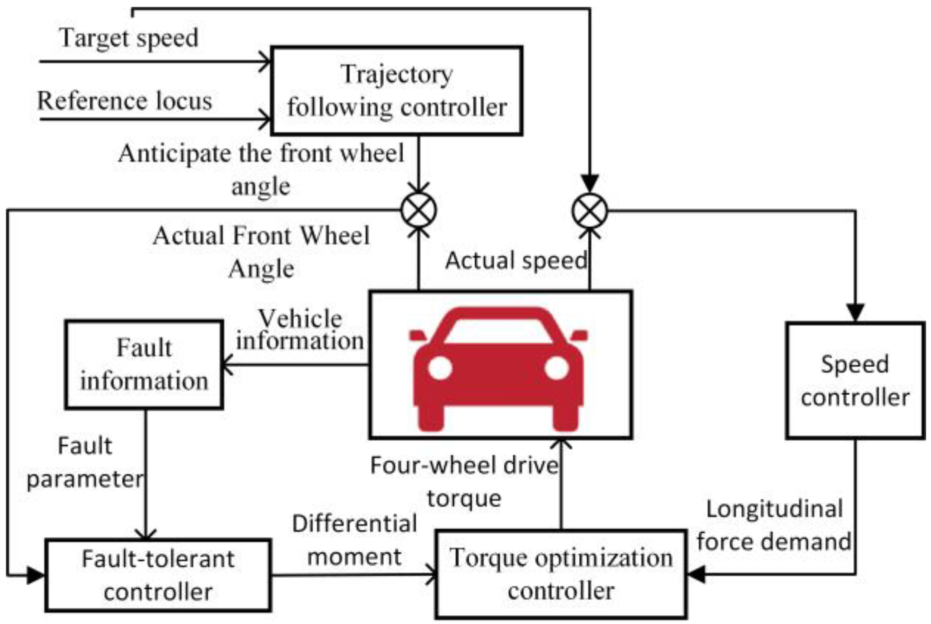
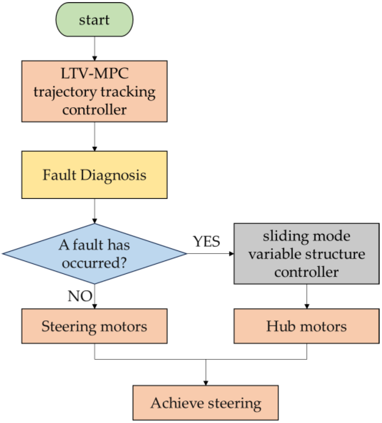
2. Control Architecture

The fault-tolerant control principle for the actuators of the proposed four-wheel independent steer-by-wire electric vehicle is illustrated in Figure 1. In the event of steer-by-wire system failure or partial loss of steering capability due to actuator malfunction, the steering failure-tolerance controller generates differential torque and transmits it to the torque distribution controller. Additionally, if the drive system fault detector identifies a fault in the drive system actuator, it sends the fault parameters to the torque distribution controller. Upon receiving this information, the torque distribution controller optimally distributes torque to each wheel to ensure optimal vehicle trajectory tracking. To achieve superior control performance, the trajectory tracking controller utilizes a model predictive control (MPC) algorithm.

When the steering system operates normally, the actuator of the steer-by-wire system can directly track the desired front wheel angle obtained through optimization and solution by the MPC trajectory tracking strategy. At this point, since the desired front wheel angle is the same as the actual front wheel angle, there is no differential torque. When the steer-by-wire system malfunctions, the front wheel angle tracking control strategy can achieve front wheel steering by generating differential torque through the distribution of front wheel drive torque. Thus, there is no need to switch the control strategy before and after the fault occurs, and the vehicle’s trajectory tracking capability and yaw stability can still be ensured after the steering system fails in Figure 2.

3. Design of the Upper-Level Trajectory Tracking Controller

3.1. Linear Time-Varying Model Predictive Control

The model predictive control (MPC) methodology consists of three essential stages: predictive modeling, iterative optimization, and feedback-based error correction. Since an optimization solution is required within each sampling period, the computational amount is considerable. Linear time-varying model predictive control can approximately linearize the nonlinear vehicle dynamics model in each sampling period, thereby being capable of enhancing the real-time performance of the algorithm while guaranteeing the control effect [21].

3.1.1. The Model of Vehicle Dynamics

Regarding the trajectory tracking issue of four-wheel hub motor-driven intelligent electric vehicles in the event of steering failure. The vehicle’s pitching motion about the y-axis and rolling motion around the x-axis are disregarded. Instead, consideration is given solely to the longitudinal, lateral, and yaw dynamics. The schematic diagram of the planar motion of the vehicle is depicted as shown in Figure 3.

The vehicle dynamic equilibrium equation is

$$m\left(\ddot{x}-\dot{y}\dot{\psi }\right)=\left(F_{xfl}+F_{xfr}\right)\cos {\delta }_f-\left(F_{yfl}+F_{yfr}\right)\sin {\delta }_f+\left(F_{xrl}+F_{xrr}\right)$$

(1)

$$m\left(\ddot{y}+\dot{x}\dot{\psi }\right)=\left(F_{xfl}+F_{xfr}\right)\sin {\delta }_f+\left(F_{yfl}+F_{yfr}\right)\cos {\delta }_f+\left(F_{yrl}+F_{yrr}\right)$$

(2)

$$\begin{array}{l}{I}_z\ddot{\psi }=l_f\left(\left(F_{xfl}+F_{xfr}\right)\sin {\delta }_f+\left(F_{yfl}+F_{yfr}\right)\cos {\delta }_f\right)\\ -l_r\left(\left(F_{xfl}+F_{xfr}\right)\sin {\delta }_f+\left(F_{yfl}+F_{yfr}\right)\cos {\delta }_f\right)+\mathrm{\Delta }{M}_z\end{array}$$

(3)

In the equation, $m$ denotes the mass of the entire vehicle; variables $x$ and $y$ denote the vehicle’s longitudinal and lateral displacements within its coordinate system, respectively, while $\psi$ represents its yaw angle; $F_{xfl}$, $F_{xfr}$, $F_{xrl}$ and $F_{xrr}$ denote the longitudinal forces acting on the four wheels, while $F_{yfl}$, $F_{yfr}$, $F_{yrl}$ and $F_{yrr}$ represent the corresponding lateral forces. The variable ${\delta }_f$ signifies the steering angle of the front wheels, whereas $I_z$ corresponds to the vehicle’s rotational inertia about the z-axis. $l_f$ and $l_r$ indicate the distances from the center of mass to the front and rear axles, respectively, and $\mathrm{\Delta }{M}_z$ represents the additional yaw moment.

In this paper, the “Magic Formula” tire model is adopted. This model employs a combination of trigonometric functions to approximate tire test data, thereby deriving a mathematical representation of the tire force. It features a unified structural form and high calculation accuracy. Moreover, it retains a relatively high level of model accuracy even under conditions involving significant slip ratios and large sideslip angles [22]. The following formula represents the longitudinal force of the tire:

$$F_{xij}=D_x\sin \left\{C_x\arctan \left[B_{x}s-E_x\left(B_{x}s-\arctan \left(B_{x}s\right)\right)\right]\right\}$$

(4)

$$C_x=a_0{D}_x=a_1{F}_z^2+a_2{F}_z$$

(5)

$$B_x=\left(a_3{F}_z^2+a_4{F}_z\right)\exp {\left(-a_{5}F\right)}_z/\left(C_x{D}_x\right)$$

(6)

$$E_x=a_6{F}_z^2+a_7{F}_z+a_8$$

(7)

Herein, ij = fl, fr, rl, rr denote the left-front, right-front, left-rear, and right-rear tires, respectively. The longitudinal force on the wheels is Fxij, while ss denotes the tire’s longitudinal slip ratio. Additionally, Fz signifies the vertical load on the tire. The coefficients a₀ to a₈ are the fitting parameters of the tire model, with their specific values listed in

Table 1. Fitting parameters of the magic tire model for longitudinal and lateral forces unit: %.

a0	a1	a2	a3	a4	a5	a6	a7	a8
1.406	−8.759	1011.783	8.062	34,788.69	0.022	−0.006	0.096	0.272
b0	b1	b2	b3	b4	b5	b6	b7	b8
1.412	−10	1025.022	3906	2	0.039	8.168 × 10−6	3.495 × 10−4	−0.282

.

The lateral force of the tire under pure sideslip conditions is expressed as follows:

$$F_{yij}=D_y\sin \left\{C_y\arctan \left[B_y\alpha -E_y\left(B_y\alpha -\arctan \left(B_y\alpha \right)\right)\right]\right\}$$

(8)

$$C_y=b_0{D}_y=b_1{F}_z^2+b_{2}F$$

(9)

$$B_y=b_3\sin \left(b_4\arctan \left(b_5{F}_z\right)\right)/\left(C_y{D}_y\right)$$

(10)

$$E_y=b_6{F}_z^2+b_7{F}_z+b$$

(11)

In the equation, F_yij represents the lateral force acting on each wheel, while α denotes the tire’s sideslip angle. Table 1 presents the tire fitting parameters.

When the tire slips under adverse circumstances [23], the longitudinal force and lateral force of the tire are

$$\begin{array}{l}{F}_{xij}={\displaystyle \frac{-s}{\sqrt{s^2+{\left(\tan \alpha \right)}^2}}}\mu D_x\sin \left\{\left({\displaystyle \frac{5}{4}}-{\displaystyle \frac{\mu }{4}}\right)C_x\times \right.\arctan \left[\left(2-\mu \right)B_{x}s-E_x\left(\left(2-\mu \right)B_{x}s\right)-\right.\\ \left.\left.\left.\arctan \left(\left(2-\mu \right)B_{x}s\right)\right)\right)\right\}\end{array}$$

(12)

$$\begin{array}{l}{F}_{yij}={\displaystyle \frac{-\tan \alpha }{\sqrt{s^2+{\left(\tan \alpha \right)}^2}}}\mu D_y\sin \left\{\left({\displaystyle \frac{5}{4}}-{\displaystyle \frac{\mu }{4}}\right)C_y\times \right.\arctan \left[\left(2-\mu \right)B_y\alpha -E_y\left(\left(2-\mu \right)B_y\alpha -\right.\right.\\ \left.\left.\left.\arctan \left(\left(2-\mu \right)B_y\alpha \right)\right)\right)\right\}\end{array}$$

(13)

In the equation, μ is the road adhesion coefficient.

The longitudinal slip ratios of each tire of the wheels are represented as

$$s_{ij}=\left\{\begin{array}{l}\left(1-{\displaystyle \frac{u_{ij}}{{\omega }_{ij}r}}\right)\times 100\%>0{\omega }_{ij}r⩾u_{ij}\hfill \\ \left({\displaystyle \frac{{\omega }_{ij}r}{u_{ij}}}-1\right)\times 100\%<0{\omega }_{ij}r<u_{ij}\hfill \end{array}\right.$$

(14)

In the equation, u_ij stands for the speed of the wheel center of each wheel, and its calculation formula is as follows:

$$u_{fl}=({\nu }_x-{\displaystyle \frac{1}{2}}{B}_f\cdot \dot{\psi })\cdot \cos {\delta }_f+({\nu }_y+l_f\cdot \dot{\psi })\cdot \sin {\delta }_f$$

(15)

$$u_{fr}=({\nu }_x+{\displaystyle \frac{1}{2}}{B}_f\cdot \dot{\psi })\cdot \cos {\delta }_f+({\nu }_y+l_f\cdot \dot{\psi })\cdot \sin {\delta }_f$$

(16)

$$u_{rl}={\nu }_x-{\displaystyle \frac{1}{2}}{B}_r\cdot \dot{\psi }$$

(17)

$$u_{rr}={\nu }_x+{\displaystyle \frac{1}{2}}{B}_r\cdot \dot{\psi }$$

(18)

The tire side slip angles of each wheel can be represented as

$${\alpha }_{fl}={\delta }_f-\arctan \left({\displaystyle \frac{{\nu }_y+l_f\cdot \dot{\psi }}{{\nu }_x-\frac{1}{2}{B}_f\cdot \dot{\psi }}}\right)$$

(19)

$${\alpha }_{fr}={\delta }_f-\arctan \left({\displaystyle \frac{{\nu }_y+l_f\cdot \dot{\psi }}{{\nu }_x+\frac{1}{2}{B}_f\cdot \dot{\psi }}}\right)$$

(20)

$${\alpha }_{rl}=\arctan \left({\displaystyle \frac{l_r\cdot \dot{\psi }-{\nu }_y}{{\nu }_x-\frac{1}{2}{B}_r\cdot \dot{\psi }}}\right)$$

(21)

$${\alpha }_{rr}=\arctan \left({\displaystyle \frac{l_r\cdot \dot{\psi }-{\nu }_y}{{\nu }_x+\frac{1}{2}{B}_r\cdot \dot{\psi }}}\right)$$

(22)

The vertical loads of each wheel are represented as

$$F_{zfl}={\displaystyle \frac{mg{l}_r}{2(l_f+l_r)}}-{\displaystyle \frac{m{a}_{x}h}{2(l_f+l_r)}}-{\displaystyle \frac{m{a}_{y}h{l}_r}{(l_f+l_r)B_f}}$$

(23)

$$F_{zfr}={\displaystyle \frac{mg{l}_r}{2(l_f+l_r)}}-{\displaystyle \frac{m{a}_{x}h}{2(l_f+l_r)}}+{\displaystyle \frac{m{a}_{y}h{l}_r}{(l_f+l_r)B_f}}$$

(24)

$$F_{zfl}={\displaystyle \frac{mg{l}_f}{2(l_f+l_r)}}+{\displaystyle \frac{m{a}_{x}h}{2(l_f+l_r)}}-{\displaystyle \frac{m{a}_{y}h{l}_f}{(l_f+l_r)B_r}}$$

(25)

$$F_{zfl}={\displaystyle \frac{mg{l}_f}{2(l_f+l_r)}}+{\displaystyle \frac{m{a}_{x}h}{2(l_f+l_r)}}+{\displaystyle \frac{m{a}_{y}h{l}_f}{(l_f+l_r)B_r}}$$

(26)

In the equation, F_ij denotes the vertical load, while a_x and a_y, respectively, represent the longitudinal acceleration and the transverse acceleration.

Transforming the vehicle coordinate system into the geodetic coordinate system, namely

$$\dot{X}=\dot{x}\cos \psi -\dot{y}\sin \psi$$

(27)

$$\dot{Y}=\dot{x}\sin \psi +\dot{y}\cos \psi$$

(28)

In the geodetic coordinate system, X denotes the longitudinal displacement of the vehicle, and Y denotes the lateral displacement.

To sum up, the vehicle lateral dynamics model can be simplified as

$$\ddot{x}=\dot{y}\dot{\psi }+{\displaystyle \frac{1}{m}}\left[F_{xfl}+F_{xfr}-\left(F_{yfl}+F_{yfr}\right){\delta }_f+F_{xrl}+F_{xrr}\right]$$

(29)

$$\ddot{y}=-\dot{x}\dot{\psi }+{\displaystyle \frac{1}{m}}\left[\left(F_{xfl}+F_{xfr}\right){\delta }_f+F_{yfl}+F_{yfr}+F_{yrl}+F_{yrr}\right]$$

(30)

$$\ddot{\psi }={\displaystyle \frac{1}{I_z}}\left[l_f\left(\left(F_{xfl}+F_{xfr}\right){\delta }_f+F_{yfl}+F_{yfr}\right)-\right.\left.l_r\left(\left(F_{xfl}+F_{xfr}\right){\delta }_f+F_{yfl}+F_{yfr}\right)\right]+{\displaystyle \frac{\mathrm{\Delta }{M}_z}{I_z}}$$

(31)

$$\dot{\psi }=\dot{\psi }$$

(32)

$$\dot{X}=\dot{x}\cos \psi -\dot{y}\sin \psi$$

(33)

$$\dot{Y}=\dot{x}\sin \psi +\dot{y}\cos \psi$$

(34)

The state-space expression of the system can be concisely written as

$$\dot{\xi }(t)=f(\xi (t),u(t))$$

(35)

$$y=C\xi (t)$$

(36)

Select $\xi ={(\dot{x},\dot{y},\dot{\psi },\psi ,X,Y)}^{\mathrm{T}}$ as the system state quantities; select $u=({\delta }_f,\mathsf{\Delta }{M}_z)$ as the system control quantities, among which δ_f indicates the virtual control quantity. In the case of system failure, the front wheel steering angle serves as a critical parameter for maintaining vehicle performance. select $y=(\psi ,\dot{\psi },Y)$ as the system output quantities.

3.1.2. Model Predictive Trajectory Tracking Control

In this section, a linear time-varying model predictive control (MPC) is designed to guide the 4WS vehicle along the reference path. In order to guarantee that the system is capable of conducting fault-tolerant control via hub motors when facing steering motor faults, the controller will additionally output the additional yaw moment necessary for maintaining vehicle body stability. When the steering motor malfunctions and fails to meet the steering requirements, differential steering will be implemented through the hub motors to fulfill the steering demands. The nonlinear model and complex objective constraints are difficult to solve for intelligent vehicles, so the system vehicle dynamics model is linearized into state space form.

$${\dot{x}}_c=A_c{x}_c+B_c{u}_c$$

(37)

$$y_c=C_c{x}_c$$

(38)

In the formula, $x_c={(v_x,v_y,\phi ,\stackrel{.}{\phi },X,Y)}^{\mathrm{T}}$ is selected as the system state variable, among which the number of system state variables N_x = 6. $u_c=\left[\begin{array}{c}{\delta }_f\end{array}\right]$ is chosen as the system control variable, among which the number of system state variables N_u = 1. Keep the longitudinal velocity constant.

$$A_c=\left(\begin{array}{cccccc}{a}_{11}& a_{12}& 0& a_{14}& 0& 0\\ a_{21}& a_{22}& 0& a_{24}& 0& 0\\ 0& 0& 0& a_{34}& 0& 0\\ a_{41}& a_{42}& 0& a_{44}& 0& 0\\ a_{51}& a_{52}& a_{53}& 0& 0& 0\\ a_{61}& a_{62}& a_{63}& 0& 0& 0\end{array}\right)$$

(39)

$$a_{11}={\displaystyle \frac{2C_{cf}{\delta }_{f,t-1}\left(v_y+a\dot{\phi }\right)}{m{v}_x^2}},a_{12}=\dot{\phi }-{\displaystyle \frac{2C_{cf}{\delta }_f}{m{v}_x}}{a}_{14}={\dot{v}}_y-{\displaystyle \frac{2C_{cf}a{\delta }_f}{m{v}_x}},$$

(40)

$$a_{22}={\displaystyle \frac{2C_{cf}-2C_{cr}}{m{v}_x}},a_{21}=-\dot{\phi }-{\displaystyle \frac{2C_{cf}\left(v_y+a\dot{\phi }\right)+2C_{cr}\left(-v_y+b\dot{\phi }\right)}{m{v}_x^2}},$$

(41)

$$a_{34}=1,a_{24}=-v_x+{\displaystyle \frac{2\left(C_{cf}a+C_{cr}b\right)}{m{v}_x}},a_{42}={\displaystyle \frac{2a{C}_{cf}+2b{C}_{cr}}{I_z{v}_x}},$$

(42)

$$a_{41}={\displaystyle \frac{2b{C}_{cr}\left(b\dot{\phi }-v_y\right)-2a{C}_{cf}\left(v_y+a\dot{\phi }\right)}{I_z{v}_x^2}},a_{44}={\displaystyle \frac{2\left(C_{cf}{a}^2-C_{cr}{b}^2\right)}{I_z{v}_x}},$$

(43)

$$a_{44}={\displaystyle \frac{2\left(C_{cf}{a}^2-C_{cr}{b}^2\right)}{I_z{v}_x}},a_{51}=\cos \phi ,a_{52}=-\sin \phi ,$$

(44)

$$a_{53}=-v_x\sin \phi -v_y\cos \phi ,a_{61}=\sin \phi ,a_{62}=\cos \phi ,a_{63}=v_x\cos \phi -v_y\sin \phi ,$$

(45)

$$B_c=\left(\begin{array}{c}{\displaystyle \frac{2C_{cf}\left(2{\delta }_f-\frac{v_Y+a\dot{\phi }}{v_X}\right)}{m}}\\ {\displaystyle \frac{2\left(C_{lf}{s}_f-C_{cf}\right)}{m}}\\ 0\\ {\displaystyle \frac{2a\left(C_{lf}{s}_f-C_{cf}\right)}{I_z}}\\ 0\\ 0\end{array}\right)$$

(46)

$$C_c={\left[\begin{array}{cccccc}0& 0& 1& 0& 0& 0\\ 0& 0& 0& 0& 0& 1\end{array}\right]}^T$$

(47)

Equations (37) and (38) are transformed into a discrete linear time-varying system with a sampling time T = 1 ms, which can be represented as follows:

$$x(k+1)=A_{k}x(k)+B_{k}u(k)$$

(48)

$$y(k)=C_{k}x(k)$$

(49)

where

$$A_k=e^{A_c{T}_s}$$

(50)

$$B_k={\displaystyle {\int }_0^{T_s}{e}^{A_{c}t}dt+B_c}$$

(51)

$$C_k=C_c$$

(52)

Define a new state variable of this discrete system

$$\zeta \left(k\right)=\left[\begin{array}{c}x\left(k\right)\\ u\left(k-1\right)\end{array}\right]$$

(53)

In order to adopt the control increment ∆u(k) as the input variable, redefine the state equation of the system so as to adapt to this new input variable:

$$\zeta (k+1)={\tilde{A}}_k\zeta (k)+{\tilde{B}}_k(u(k)-u(k-1))$$

(54)

$$Y(k)={\tilde{C}}_k\zeta (k)$$

(55)

where

$$A=\left[\begin{array}{cc}{A}_k& B_k\\ 0_{1\times 6}& I\end{array}\right],B=\left[\begin{array}{c}{B}_k\\ I\end{array}\right],C=\left[\begin{array}{ll}{C}_k\hfill & 0\hfill \end{array}\right]$$

(56)

3.1.3. Optimal Motion Control

In order to realize the prediction of vehicle states, handle constraint conditions, and optimize control inputs, thereby improving the stability and safety of the vehicle, the performance metrics are designed as

$$\begin{array}{l}J(\zeta (k),u(k-1),\mathsf{\Delta }U(k))\\ =\sum _{i=1}^{N_{\mathrm{p}}}Y(k+i|k)-Y_{\mathrm{ref}}{(k+i|k)}_{{\mathrm{Q}}_{\mathrm{m}}}^2\\ +\sum _{i=1}^{N_{\mathrm{c}}-1}\mathsf{\Delta }u{(k+i|k)}_{R_{\mathrm{m}}}^2+\rho {\kappa }^2\end{array}$$

(57)

The first item of the optimization objective function is targeted at minimizing the heading angle deviation and lateral deviation from the desired trajectory for tracking; the second item sets minimizing the variation in the control quantity as the optimization objective, considering that an overly large turning angle might lead to the vehicle being out-of-control. Q_m and R_m are, respectively, the weight matrices for trajectory tracking accuracy and control increment. In this paper:

$$Q_m\in R^{3\times 3},Q_m=\left(\begin{array}{ccc}200& 0& 0\\ 0& 10& 0\\ 0& 0& 100\end{array}\right)$$

(58)

$$R_m\in R^{2\times 2},R_m=\left(\begin{array}{cc}50000& 0\\ 0& 10\end{array}\right)$$

(59)

To avoid the sudden change in the system control quantity that might affect its continuity, a relaxation factor k is incorporated. Taking into account the constraints on the control quantity imposed by the mechanical structure and kinematics, the constraints on the control increment, control quantity, and system output are presented as follows:

$${\underset{\mathrm{\Delta }U\left(k\right),}{\min }}_{\epsilon }J\left(\zeta \left(k\right),u\left(k-1\right),\mathrm{\Delta }U\left(k\right)\right)$$

(60)

$$\begin{array}{l}s.t.(\mathrm{\Delta }{\mathrm{U}}_{\min }\le \mathrm{\Delta }U\left(k\right)\le u_{\max }\\ U_{\min }\le A\mathrm{\Delta }{U}_k+U_k\le U_{\max }\\ y_{h.\min }\le y_h\le y_{h.\max }\\ y_{s.\min }-\epsilon \le y_s\le y_{s.\mathrm{ma}}+kk>0\end{array}$$

(61)

By solving Formulas (37) and (38) within each control time domain, a sequence of optimal control increments can be derived:

$$\mathsf{\Delta }{U}^{\ast }={[\mathsf{\Delta }u(k),\mathsf{\Delta }u(k+1),\dots ,\mathsf{\Delta }u(k+H_c-1)]}^T$$

(62)

Select the first control element from this control sequence and apply it to the system to obtain the optimal control quantity at the current instant

$$U(k)=u(k-1)+\mathsf{\Delta }{u}^{\ast }(k)$$

(63)

In the equation, $\mathsf{\Delta }{u}^{\ast }(k)$ precisely represents the increment of the front wheel angle f that is required to be solved. The predicted control quantity is exerted on the system. The additional yaw moment $\mathrm{\Delta }{M}_z$ is directly fed into the lower-level torque optimization distribution layer.

3.2. The Design of Corner Controller

For the four-wheel independent steer-by-wire electric vehicle investigated in this study, each wheel is equipped with a hub motor. The driver’s input is transmitted to the electronic control unit (ECU) via the steering wheel, and the ECU processes this input along with other sensor data to command the hub motors on both the front and rear axles, thereby achieving differential steering. In this research, the differential steering mechanisms on both the front and rear axles are identical, as illustrated in Figure 4.

The dynamic equation of the differential steering system can be represented by the following formula:

$$J_i{\ddot{\delta }}_i+b_i{\dot{\delta }}_i={\tau }_{ai}+M_i^{\prime }-{\tau }_{fi}$$

(64)

wherein, $J_i\left(i=f,r\right)$ denotes the effective rotational inertia of the front/rear differential steering system, ${\delta }_i\left(i=f,r\right)$ represents the front/rear wheel steering angles of the vehicle, $b_i\left(i=f,r\right)$ stands for the effective damping of the front/rear differential steering system, ${\tau }_{fi}\left(i=f,r\right)$ is the friction torque of the front/rear differential steering system, and $M_i^{\prime }\left(i=f,r\right)$ represents the difference in the steering torques around the respective kingpins of the left and right wheels on the front/rear axle.

When the side slip angle of the tire ${\alpha }_i$ is far less than the sliding side slip angle ${\alpha }_{sli}\left({\alpha }_{sli}=\arctan (1/{\theta }_{yi}\right)$, ${\theta }_{yi}=2k_{pi}{l}^2/3\mu F_{Zi}$, the aligning torque exerted by the ground on the tire can be represented as [24]:

$${\tau }_{ai}=\mu F_{Zi}l{\theta }_{yi}{\sigma }_{yi}\left[1-3\left|{\theta }_{yi}{\sigma }_{yi}\right|+3{\left({\theta }_{yi}{\sigma }_{yi}\right)}^2-{\left|{\theta }_{yi}{\sigma }_{yi}\right|}^3\right]$$

(65)

wherein, $\mu$ is the road adhesion coefficient, l is half of the tire trailing distance, $k_{pi}$ is the tire cornering stiffness coefficient per unit length, and $k_{pi}=k_i/(2l)$.

When the tire side slip angle is very small, it follows that:

$${\tau }_{ai}=k{k}_i{\alpha }_i$$

(66)

wherein, $k=l^2/3$.

In order to simplify the dynamic model of the differential steering system, considering that the second derivative of the wheel angle ${\stackrel{..}{\delta }}_i$ and the friction torque of the steering system ${\tau }_{fi}$, are generally very small, these minor disturbances are disregarded in the modeling process. As a result, the dynamic model of the differential steering system can be further simplified.

$$b_i{\dot{\delta }}_i={\tau }_{ai}+M_i^{\prime }$$

(67)

Herein, the difference in the steering torque $M_i^{\prime }$ of the left and right front wheels around the kingpin axis can be computed based on the following formula:

$$M_i^{\prime }=\left(F_{xir}-F_{xil}\right)r_{\sigma }$$

(68)

Due to the variance of longitudinal driving forces, the resulting yaw moment can be defined as

$$\mathsf{\Delta }{M}_i=(F_{xir}-F_{xil})l_s$$

(69)

Among them, l_s is half of the track width between the left and right wheels on the same axle.

By integrating Formulas (68) and (69), it can be obtained that:

$$M_i^{\prime }={\displaystyle \frac{r_{\sigma }}{l_s}}\mathsf{\Delta }{M}_f$$

(70)

Based on the aforementioned formula, it can be derived that:

$${\dot{\delta }}_f={\displaystyle \frac{1}{b_{eff}}}({\tau }_a+M_f^{\prime })$$

(71)

Construct the sliding mode surface switching function so as to enhance the tracking effect of the front wheel angle.

$$s={\delta }_{fd}-{\delta }_f$$

(72)

The differentiation of the sliding mode surface leads to

$$\dot{s}={\dot{\delta }}_{fd}-{\dot{\delta }}_f={\dot{\delta }}_{fd}-{\displaystyle \frac{1}{b_{eff}}}({\tau }_a+M_f^{\prime })$$

(73)

Employing the exponential reaching law, there is

$$\dot{s}=-\epsilon \mathrm{sgn}(s)-ks\epsilon >0k>0$$

(74)

Combined with Equation (27), it can be obtained

$${\dot{\delta }}_{fd}-{\displaystyle \frac{1}{b_{eff}}}({\tau }_a+M_f^{\prime })=-\epsilon \mathrm{sgn}(s)-ks$$

(75)

Then, the sliding mode control rate is

$$M_f^{\prime }=b_{eff}({\dot{\delta }}_{fd}+\epsilon \mathrm{sgn}(s)+ks)-{\tau }_a$$

(76)

To restrain the chattering phenomenon resulting from model uncertainties and external interferences, the saturation function $\mathrm{sat}\left(s\right)$ is utilized to substitute the sign function $\mathrm{sgn}\left(s\right)$, namely

$$\mathrm{sat}\left(s\right)=\left\{\begin{array}{ll}1\hfill & s>\mathrm{\Delta }\hfill \\ -ks\hfill & \left|s\right|\le \mathrm{\Delta }\hfill \\ -1\hfill & s<-\mathrm{\Delta }\hfill \end{array}k=1/\mathrm{\Delta }\right.$$

(77)

In the equation, Δ is the thickness of the boundary layer of the sliding mode surface.

4. The Design of the Lower-Level Torque Optimization Distribution Controller

The size of the tire force is constrained by the vertical load of the tire. In order to avoid a severe overload of a certain tire during the vehicle’s movement, which thereby affects the vehicle’s ultimate performance, in this paper, the objective is to minimize the tire load ratio. Moreover, it satisfies the yaw moment $\mathrm{\Delta }{M}_z$, the differential moment $M_f^{\prime }$, and the longitudinal driving force $F_{xd}$ necessary for the upper-level trajectory tracking and enhancing the stability margin of the vehicle. The objective function is presented as follows:

$$\min J=\min \sum _{ij=fl,fr,rl,rr}{\displaystyle \frac{c_{ij}{F}_{txdij}^2+s_{ij}{F}_{tydij}^2}{{\left(\mu F_{zij}\right)}^2}}$$

(78)

In the equation, $F_{txdij}$ and $F_{tydij}$ denote the optimized distributed longitudinal and lateral forces of the tires, respectively; $\mu$ represents the road adhesion coefficient; $c_{ij}$, $s_{ij}$ are the distribution weight coefficients of the longitudinal and lateral forces of the tires, respectively, which are used to adjust the proportion of the tire forces in the optimization objective function. Under normal driving conditions, $c_{ij}=s_{ij}=1$.

On the one hand, the distributed tire forces need to satisfy the longitudinal force, lateral force, and yaw moment demanded by the upper-level controller. On the other hand, the maximum output torque of the hub motor and the constraints of road adhesion conditions also need to be considered. Hence, the constraint conditions are as follows:

$$\sum _{ij=fl,fr,rl,rr}{F}_{txdij}\cos {\delta }_{ij}-\sum _{ij=fl,fr,rl,rr}{F}_{tydij}\sin {\delta }_{ij}=F_{xd}$$

(79)

$$\sum _{ij=fl,fr,rl,rr}{F}_{txdij}\sin {\delta }_{ij}+\sum _{ij=fl,fr,rl,rr}{F}_{tydij}\cos {\delta }_{ij}=F_{yd}$$

(80)

$$\begin{array}{l}\left(-b\cos {\delta }_{fl}+l_f\sin {\delta }_{fl}\right)F_{txdfl}+\left(b\cos {\delta }_{fr}+l_f\sin {\delta }_{fr}\right)F_{txdfr}+\\ \left\{\left(-b\cos {\delta }_{rl}-l_r\sin {\delta }_{rl}\right)F_{txdrl}+\left(b\cos {\delta }_{rr}-l_r\sin {\delta }_{rr}\right)F_{txdrr}+\right.\\ \left(l_f\cos {\delta }_{fl}+b\sin {\delta }_{fl}\right)F_{tydfl}+\left(l_f\cos {\delta }_{fr}-b\sin {\delta }_{fr}\right)F_{tydfr}+\\ \left(-l_r\cos {\delta }_{rl}+b\sin {\delta }_{rl}\right)F_{tydrl}+\left(-l_r\cos {\delta }_{rr}-b\sin {\delta }_{rr}\right)F_{tydrr}=\mathrm{\Delta }{M}_z\end{array}$$

(81)

$$-T_{ij\max }\le F_{txdij}\cdot r_{ij}\le T_{ij\max }$$

(82)

$$F_{txdij}^2+F_{tydij}^2\le {\mu }^2{F}_{zij}^2$$

(83)

In the equation, $T_{ij\max }$ is the maximum output torque of the hub motor. Regarding the nonlinear inequality constraints in the constraint conditions, the approach mentioned in reference [25] is utilized, and it is approximated as a linear constraint by means of octagonal approximation.

The driving torques of each wheel are solved by means of the quadratic programming method, and the obtained performance index is

$$\begin{array}{l}J=u^T\mathrm{\Omega }u+{\left(ku-v\right)}^T\zeta \left(ku-v\right)\\ s.t.u_{\min }\le u\le u_{\max }\end{array}$$

(84)

$$\mathrm{\Omega }=\mathrm{diag}\left\{{\displaystyle \frac{1}{{\left(r_{\mathrm{w}}\mu F_{\mathrm{zfl}}\right)}^2}},{\displaystyle \frac{1}{{\left(r_{\mathrm{w}}\mu F_{\mathrm{zfr}}\right)}^2}},{\displaystyle \frac{1}{{\left(r_{\mathrm{w}}\mu F_{\mathrm{zrl}}\right)}^2}},{\displaystyle \frac{1}{{\left(r_{\mathrm{w}}\mu F_{\mathrm{zrr}}\right)}^2}}\right\}$$

(85)

$$\zeta =\mathrm{diag}\left\{{\zeta }_1,{\zeta }_2,{\zeta }_3\right\}$$

(86)

$$u=\left[T_{fl}{T}_{fr}{T}_{rl}{T}_{rr}\right]$$

(87)

wherein: Matrices $\mathrm{\Omega }$ and $\zeta$ are the weight matrix for satisfying the equation conditions; ${\zeta }_1,{\zeta }_2,{\zeta }_3$ are, respectively, the weights of the differential torque $\mathrm{\Delta }{M}_f$, the demanded longitudinal torque $T_{tot}$, and the additional yaw moment; $u$ is the optimization vector of the solver, representing the output torques of each hub motor; v is the expected values of the differential torque $\mathrm{\Delta }{M}_f$, the demanded longitudinal torque $T_{tot}$, and the additional yaw moment (which is set to 0 to avoid influencing the trajectory tracking process), namely

$$v={\left[\mathrm{\Delta }{M}_{\mathrm{f}}{T}_{\mathrm{tot}}0\right]}^T$$

(88)

K is the gain matrix and can be represented as

$$K=\left[\begin{array}{c}{\displaystyle \frac{r_{\sigma }\cos \varsigma \cos \sigma }{r_{\mathrm{w}}}}\times \left[-m_{\mathrm{fl}}{m}_{\mathrm{fr}}00\right]\\ \left[\begin{array}{llll}{m}_{\mathrm{fl}}\hfill & m_{\mathrm{fr}}\hfill & m_{\mathrm{rl}}\hfill & m_{\mathrm{rr}}\hfill \end{array}\right]\\ {\displaystyle \frac{d_{\mathrm{s}}}{2r_{\mathrm{w}}}}\times \left[-m_{\mathrm{fl}}{m}_{\mathrm{fr}}-m_{\mathrm{rl}}{m}_{\mathrm{rr}}\right]\end{array}\right]$$

(89)

5. Simulation Analysis of Typical Operating Conditions

In order to verify the effectiveness of the above fault-tolerant control strategy, experiments were carried out under single shift and double shift conditions, respectively. The experimental platform is jointly built by MATLAB/Simulink and CarSim, and the parameters of the vehicles used in the experiment are shown in

Table 2. Vehicle parameters.

Parameter	Values
Vehicle curb weight/kg	1880
The length from the center of mass to the front axle/m	1.015
The distance between the center of mass and the rear axle/m	1.895
Axis length/m	1.675
$\mathrm{Lateral}\mathrm{stiffness}\mathrm{of}\mathrm{the}\mathrm{front}\mathrm{wheel}/(N·{rad}^{-1}$)	152,500
$\mathrm{Lateral}\mathrm{stiffness}\mathrm{of}\mathrm{the}\mathrm{rear}\mathrm{wheel}/(N·{rad}^{-1}$)	135,400
Radius of the tire/m	0.33
Road surface adhesion coefficien (μ)	0.8
Boundary values of torque output of in-wheel motor/(N·m)	800

:

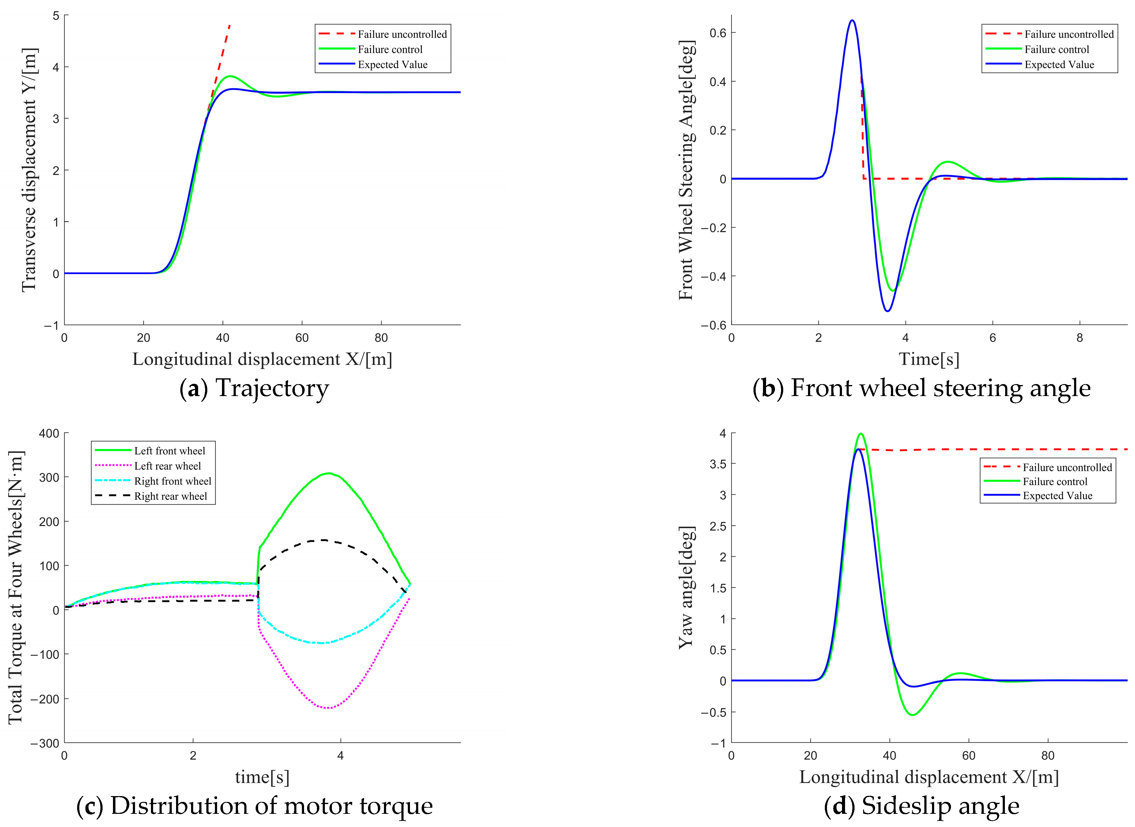
5.1. Single Shift-Line Operating Condition

To validate the fault-tolerant control approach for the actuator of the steering system presented in this paper, a step steering simulation working condition experiment was set. A step steering angle of 0.1 rad was generated at 1 s, and the actuator failure of the steering system occurred at 3 s. The experimental conditions were as follows: the speed was 100 km/h, and the road adhesion coefficient was 0.8. The simulation experiment results are depicted in Figure 5.

It can be observed that when the actuator of the steering system malfunctions at 3 s, as depicted in Figure 5e, the vehicle without fault-tolerant control loses its steering capability, and the yaw angular velocity subsequently drops to 0. The yaw angle will maintain the current value, and the vehicle will continue to travel along the course angle at the current instant. Figure 5f,g indicate that the experimental results of the vehicle with the fault-tolerant controller after the fault are approximately consistent with those of the fault-free vehicle. The maximum lateral position deviation is 0.0917 m, the average relative lateral position deviation is 5.96%, the maximum deviation of the centroid sideslip angle is 0.426°, the average relative deviation of the centroid sideslip angle is 9.3%, the maximum deviation of the yaw angular velocity is 0.227 deg/s, and the fluctuation range of the longitudinal velocity error is [0, 0.04]. As can be seen from Figure 5c, the driving torques of the four wheels are significantly different, which attests that the steering is accomplished through differential driving torques, and the torque optimization distribution controller is employed to optimize the torque distribution of the four tires. While ensuring the smooth progress of steering, the tire load rate is maintained below 30%, as can be seen from Figure 5h, providing the vehicle with a better stability margin. To sum up, the simulation results validate the effectiveness of the fault-tolerant controller for steering faults proposed in this paper.

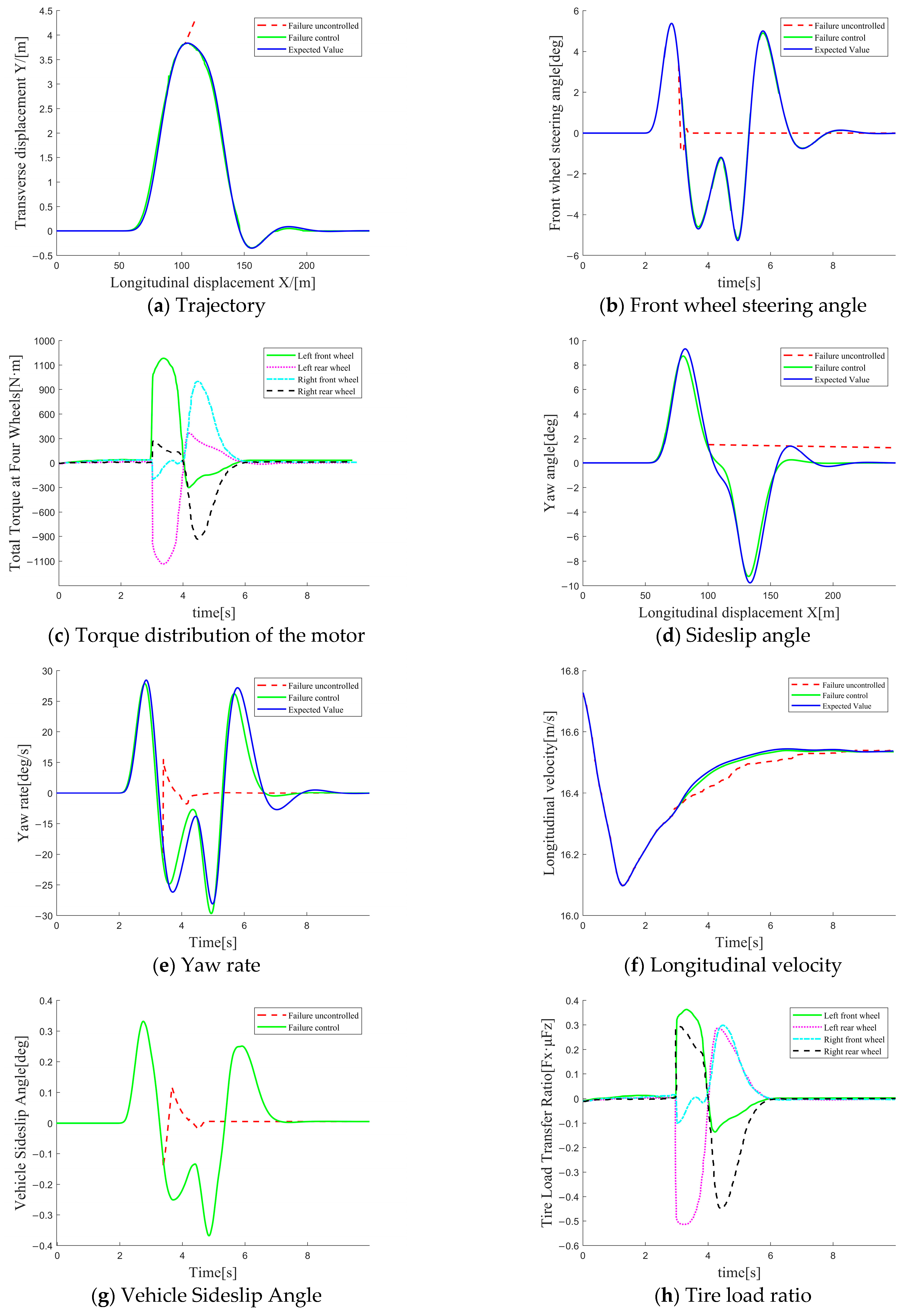
5.2. Double Shift-Line Operating Condition

To validate the effectiveness of the multi-actuator failure-tolerant control approach proposed in this paper, a double lane change operating condition experiment was conducted. The experimental conditions were as follows: the speed was 60 km/h, and the road adhesion coefficient was 0.8. The vehicle scenarios in this experiment can be categorized into three types. The first is the ideal vehicle derived from model prediction, serving as the ideal reference model. The second is the failed and uncontrolled vehicle when the actuator of the steering system fails and no fault-tolerant control is implemented. The third type is the controlled vehicle, in which the fault-tolerant control strategy put forward in this paper has been employed after the malfunction of the steering system.

Figure 6 presents the outcomes of the simulation experiments. As can be observed from Figure 6b, the vehicle lost its steering capability due to the malfunction of the steering actuator. Nevertheless, it can be discerned from Figure 6a that the fault-tolerant vehicle possesses superior trajectory tracking precision. This demonstrates the efficacy of the fault-tolerant control approach proposed in this paper for steering failure fault-tolerant control. As depicted in Figure 6c, the driving torques of the two wheels on the front axle are conspicuously dissimilar. The front wheel steering angle generated through differential steering can precisely track the reference value output by the upper-level controller. Simultaneously, direct yaw moment control is imposed to ensure that the vehicle’s yaw rate tracks the expected value. It can be observed from Figure 6d–g that when the vehicle loses its steering ability, the vehicle under fault-tolerant control is still capable of ensuring relatively good steering stability. The maximum deviation of the centroid sideslip angle is 1.746°, the average relative deviation of the centroid sideslip angle is 13.2%, the maximum deviation of the yaw rate is 0.016 deg/s, and the average relative deviation of the yaw rate is 9.75%. Figure 6h reveals that the tire load ratios of the four wheels are relatively small, providing adequate leeway for the stability control of the vehicle.

6. Conclusions

In response to the failure of the wire-controlled steering system of four-wheel independent wire-controlled steering electric vehicles, a fault-tolerant control method based on the synergy of differential steering and direct yaw moment control is proposed. In the upper-level control framework, the trajectory tracking controller based on model predictive control (LCV-MPC) computes the necessary front wheel steering angle and additional yaw moment in accordance with the pre-determined target trajectory. The controller minimizes the trajectory tracking error by optimizing the calculation outcomes, ensuring that the vehicle accurately follows the reference trajectory and is capable of adapting to environmental and dynamic variations. while implementing differential steering through sliding mode variable structure control algorithms to regulate drive motors based on target steering angles. The lower-layer torque distribution controller optimizes wheel torque allocation with the objective of minimizing tire load rates under predefined yaw moment constraints. Simulation results demonstrate that the proposed strategy reduces path tracking capability decreases by merely 3–5% under steering motor failure scenarios in single-lane-change and double-lane-change maneuvers, with sideslip angle deviation controlled within 10% and yaw rate deviation below 8%. The method ensures satisfactory steering performance with excellent real-time responsiveness.

In order to make the research more closely align with practical engineering needs, the next step in our research will involve conducting real-vehicle tests to obtain more valuable reference data and authentic experimental results.

References

1. Li, K.; Chen, T.; Luo, Y.; Wang, J. Intelligent Environment-Friendly Vehicles: Concept and Case Studies. IEEE Trans. Intell. Transp. Syst. 2012, 13, 318–328. [Google Scholar] [CrossRef]
2. Qu, X.; Pi, D.; Zhang, L.; Lv, C. Advancements on unmanned vehicles in the transportation system. Green Energy Intell. Transp. 2023, 2, 100091. [Google Scholar] [CrossRef]
3. Mortazavizadeh, S.A.; Ghaderi, A.; Ebrahimi, M.; Hajian, M. Recent Developments in the Vehicle Steer-by-Wire System. IEEE Trans. Transp. Electrif. 2020, 6, 1226–1235. [Google Scholar] [CrossRef]
4. Zong, C.; Li, G.; Zhang, H.; He, L.; Zhang, Z. Study progress and outlook of chassis control technology for X-by-wire automobile. China J. Highw. Transp. 2013, 26, 160–176. [Google Scholar]
5. Zhang, X.; Cocquempot, V. Fault tolerant control scheme based on active fault diagnosis for the path tracking control of a 4WD electric vehicle. In Proceedings of the 2014 IEEE International Symposium on Intelligent Control (ISIC), Juan Les Pins, France, 8–10 October 2017; pp. 2189–2195. [Google Scholar]
6. Hasan, M.; Anwar, S. Sliding Mode Observer and Long Range Prediction Based Fault Tolerant Control of a Steer-by-Wire Equipped Vehicle. SAE Tech. Pap. 2008, 41, 8534–8539. [Google Scholar]
7. Shi, G.B.; Guo, C.; Wang, S.; Liu, T.Y. Angle Tracking and Fault-Tolerant Control of Steer-by-Wire System with Dual Three-Phase Motor for Autonomous Vehicle. IEEE Trans. Intell. Transp. Syst. 2024, 25, 5842–5853. [Google Scholar] [CrossRef]
8. Yang, K.; Kang, D.; Lee, D. Fault tolerant control using self-diagnostic smart actuator. In Proceedings of the 2009 ICCAS-SICE, Fukuoka, Japan, 18–21 August 2009; pp. 5674–5678. [Google Scholar]
9. Zhang, B.; Lu, S. Fault-tolerant control for four-wheel independent actuated electric vehicle using feedback linearization and cooperative game theory. Control. Eng. Pract. 2020, 101, 104510. [Google Scholar] [CrossRef]
10. Li, H.; Zhang, N.; Wu, G.; Li, Z.; Ding, H.; Jiang, C. Active Fault-Tolerant Control of a Four-Wheel Independent Steering System Based on the Multi-Agent Approach. Electronics 2024, 13, 748. [Google Scholar] [CrossRef]
11. Meléndez-Useros, M.; Viadero-Monasterio, F.; Jiménez-Salas, M.; López-Boada, M.J. Static Output-Feedback Path-Tracking Controller Tolerant to Steering Actuator Faults for Distributed Driven Electric Vehicles. World Electr. 2025, 16, 40. [Google Scholar] [CrossRef]
12. Im, J.S.; Ozaki, F.; Yeu, T.K.; Kawaji, S. Model-based fault detection and isolation in steer-by-wire vehicle using sliding mode observer. J. Mech. Sci. Technol. 2009, 23, 1991–1999. [Google Scholar] [CrossRef]
13. Huang, C.; Naghdy, F.; Du, H. Delta Operator Based Fault Detection Filter Design for Uncertain Steer-by-Wire Systems with Time Delay. In Proceedings of the 2018 Chinese Control Conference (CCC), Wuhan, China, 25–27 July 2018; pp. 7730–7735. [Google Scholar]
14. Chen, T.; Cai, Y.; Chen, L.; Xu, X.; Sun, X. Trajectory tracking control of steer-by-wire autonomous ground vehicle considering the complete failure of vehicle steering motor. Simul. Model. Pract. Theory 2021, 109, 102235. [Google Scholar] [CrossRef]
15. Seiffer, A.; Schütz, L.; Frey, M.; Gauterin, F. Constrained Control Allocation Improving Fault Tolerance of a Four Wheel Independently Driven Articulated Vehicle. IEEE Open J. Intell. Transp. Syst. 2023, 4, 187–203. [Google Scholar] [CrossRef]
16. Luo, Y.; Chen, R.; Hu, Y. Active fault-tolerant control based on MFAC or 4WID EV with steering by wire system. J. Mech. Eng. 2019, 55, 131–139. [Google Scholar]
17. Asperti, M.; Vignati, M.; Sabbioni, E. Design of Electric Power Steering Control for Compensating the Torque Steer Effect due to Torque Vectoring Control. SAE Int. J. Veh. Dyn. Stab. NVH 2025, 9, 17. [Google Scholar] [CrossRef]
18. Jo, S.-J.; Baek, S.-W.; Hwang, K.-Y. Optimization Design of Novel Consequent Pole Motor for Electric Power Steering System. Machines 2024, 12, 893. [Google Scholar] [CrossRef]
19. Zhu, S.; Lu, J.; Zhu, L.; Chen, H.; Gao, J.; Xie, W. Coordinated Control of Differential Drive-Assist Steering and Direct Yaw Moment Control for Distributed-Drive Electric Vehicles. Electronics 2024, 13, 3711. [Google Scholar] [CrossRef]
20. Hu, C.; Wang, R.; Yan, F. Differential steering based yaw stabilization using ISMC for independently actuated electric vehicles. IEEE Trans. Intell. Transp. Syst. 2018, 19, 627–638. [Google Scholar] [CrossRef]
21. Xin, P.; Wang, Z.; Sun, H.; Zhang, B. Model Predictive Control of Unmanned Mine Vehicle Trajectory Tracking. In Proceedings of the 2021 Chinese Control Conference (CCC), Shanghai, China, 26–28 July 2021; pp. 4757–4762. [Google Scholar]
22. Hans, P. Tyre and Vehicle Dynamics; Butterworth-Heinemann: Oxford, UK, 2002. [Google Scholar]
23. Lu, S. Study on Vehicle Chassis Key Subsystems and Its Integrated Control Strategy; Chongqing University: Chongqing, China, 2009. [Google Scholar]
24. Wang, Q.; Wang, J.; Jin, L. Differential assisted steering applied on electric vehicle with electric motored wheels. J. Jinlin Univ. 2009, 39, 1–6. [Google Scholar]
25. Jiao, G. Study on Longitudinal and Lateral Force Coordinated Control of Four wheel Independent Driving/Steering Electric Vehicle; Chongqing University: Chongqing, China, 2018. [Google Scholar]
Figure 1. Principal diagram of fault-tolerant control method for four-wheel independent steering by wire electric vehicle.
Wevj 16 00183 g001
Figure 2. Flowchart of fault-tolerant control for four-wheel independent steering of electric vehicles.
Wevj 16 00183 g002
Figure 3. The three-degree-of-freedom vehicle model.
Wevj 16 00183 g003
Figure 4. Schematic diagram of differential steering.
Wevj 16 00183 g004
Figure 5. Simulation results of the single lane change operating condition.
Wevj 16 00183 g005aWevj 16 00183 g005b
Figure 6. Simulation results of following vehicle cruise control.
Wevj 16 00183 g006