From Map to Policy: Road Transportation Emission Mapping and Optimizing BEV Incentives for True Emission Reductions

Abstract

This study explores the importance of considering regional aspects and different calculation approaches when assessing the environmental impact of passenger cars in Germany. The transportation sector, in general, needs to improve its transition to comply with national and international goals, and more efficient measures are necessary. To achieve this, the spatial heterogeneity of underlying data, such as vehicle stocks, cubic capacity classes as a proxy for consumption values, and annual mileage, is investigated with respect to regional differences. Using data samples for the year 2017, the average emission values per car and year are calculated as well as Germany’s total emission values from the utilization of passenger cars. Conducting a spatially informed allocation algorithm, battery electric vehicles (BEVs) are added to certain regional fleets, replacing cars with internal combustion engines (ICEs). The results show significant regional differences in the underlying data, with a divergence between rural and urban areas as well as northern and southern regions, while the spread in mileage values is higher than that in consumption values. Comparing the tank-to-wheel (TtW) and well-to-wheel (WtW) approaches reveals different values with an increased spread as more BEVs are introduced to the fleet. Using the presented concept to allocate BEVs, emissions can be reduced by 1.66% to 1.35%, depending on the calculation perspective, compared to the extrapolation of historical values. Furthermore, rural areas benefit more from optimized allocation compared to urban ones. The findings suggest that regional distribution strategies could lead to more efficient reductions in GHG emissions within the transportation sector while incorporating both TtW and WtW approaches, leading to more comparable and precise analyses.

1. Introduction

With the publication of the 2024 UN Emission Gap Report, it has become clear the deviation between environmental goals and the path to reaching them has increased, stressing the need for more effective emission reduction processes. While different sectors emit greenhouses gases (GHGs) in different quantities, their mitigation potentials also differ. Regarding the transportation sector, road transportation accounts for the majority of GHG emissions [1]. In 2022, Germany produced around $754.3$ million tons of CO_2-eq., of which $144.0$ million tons or 19.1% were emitted in the road-based transportation sector by burning fossil fuels; 62% of these, or $89.5$ million tonnes, were emitted by passenger cars alone [2,3]. At the same time, the transportation sector is one of the few that has not seen significant emission reductions in recent decades, notably increasing its share of Germany’s total emissions from 16.3% in 1995 to 19.1% in 2022 [2,3]. With regard to the overall gap mentioned, decarbonizing the transportation sector is a crucial step toward mitigating climate change.

Addressing emissions from transport is particularly critical because mobility is a universal human need. It connects individuals to opportunities, resources, and experiences, playing a vital role in enhancing quality of life. However, this necessity is complex and manifests in diverse forms shaped by various factors such as socio-demographics, personal preferences, and external circumstances [4,5]. While mobility expands possibilities and brings pleasure, it also has notable downsides, including its environmental impact.

Meanwhile, the Paris Agreement has built a base for national environmental plans and contains nationally determined contributions (NDCs) created by the participating countries, some of which apply to Germany. Alongside long-term low greenhouse gas emission development strategies (LT-LEDS), these plans state the contribution of each country toward reaching the goals set by the Paris Agreement [6]. For Germany, in addition, non-binding goals such as the Klimaschutzplan 2050 (BMUB) and Klimaschutzprogramm 2030, as well as obligatory goals were set by the Klimaschutzgesetz (KSG) in 2019 [7,8,9]. In 2021, the goals were further adapted and tightened according to the judgment of the Federal Constitutional Court, leading to an intended maximum amount of 85 $\mathrm{M}$$\mathrm{t}$CO_2-eq. emissions by 2030 [10]. In 2024, a second modification was passed into law, which, besides other adaptions, changed the balancing logic from a sector-specific to a sector-overarching approach, thus avoiding sector-specific emergency measures taken in the current legislative period [11]. Projection reports, which are part of the regulatory framework of climate politics, predict a deviation from the sector target of 27.7% to 34.7% of the transportation sector goals by 2030 [12]. Even if not balanced separately, this stresses the need for further improvement in the transportation sector and raises the question of how to achieve this goal. Moreover, it should be noted that the mentioned greenhouse gas (GHG) emissions usually represent the TtW perspective. This means only tailpipe or local emissions, such as burning fuel, are covered. In contrast to this, the WtW emission perspective also covers preprocesses such as fuel refining, electricity production, and transportation, and it is usually found in scientific research but not in official statements, e.g. political reports. The goal of this work is to obtain a deeper understanding of the underlying data necessary to calculate road-based emissions and take different calculation perspectives into account. To illustrate how measures such as the introduction of BEVs can help to close the gap between the status quo and target emission values, the effect of an optimized allocation algorithm for BEVs is shown. This understanding can further help to sharpen policies, incentivizing new E-mobility by using regional aspects to achieve a more efficient transition toward a clean transportation sector.

To monitor and report progress toward environmental goals, official sites require reliable information regarding emission values. Different models are used to calculate these emissions. In the United States, MOVES (MOtor Vehicle Emission Simulator) is used by the Environmental Protection Agency (EPA) at the national and state levels [13]. Most members of the European Union (EU) use COPERT as a tool to assess emissions [14]. While most European countries acknowledge COPERT, they often have their own models, which are used for governmental decision making. In Germany, TREMOD (a Transport Emission Model) is used as a tool to calculate GHG emissions within the transportation sector [15]. The emission factors necessary for this are taken from the HBEFA (Handbook for Emission Factors for Road Transport), which is widely used in other EU countries as well [16]. TREMOD itself is not only used by governmental institutes such as the Umweltbundesamt (UBA) but also by associations, e.g., the VDA (Association of the Automotive Industry), the MWV (Mineralölwirtschaftsverband), and the Deutsche Bahn, indicating the broad acceptance of this tool [17]. TREMOD covers all means of passenger and freight transportation, not only covering GHG emissions but also carbon monoxide, hydrocarbons, nitrous oxide, and others. It differentiates emissions by road type and the mentioned means of transport; however, it does not distinguish where certain road types are [15,18].

Research examining the environmental impacts of automotive emissions encompasses a range of dimensions, including fleet-level analyses and variations in regional driving patterns and grid mixes over time. Regional variations in emissions and driving conditions play a significant role in shaping the environmental performance of vehicles. Di et al. [19] conducted a cradle-to-grave Life Cycle Assessment (LCA) that takes into account county-level driving cycles and fuel production. They pinpoint critical disparities in emissions based on distinctions between urban and highway driving, variations in regional fuel types, and temperature fluctuations. While this study follows a logic comparable to the TREMOD models, using different road types, they still offer valuable insights, stressing the need for a regionalized perspective.

In two studies, Yuksel et al. [20,21] further emphasized the significance of regional factors, particularly in relation to grid mix and climatic conditions. They also showed that ICE vehicles may outperform BEVs in areas with carbon-intensive grids, highlighting the drawbacks of singular policy approaches. Moreover, they explore the influence of temperature on BEV efficiency, range, and emissions, utilizing a US-based case study to stress the need to consider local conditions. Tamayao et al. [22] examine regional variability and uncertainty in CO_2-eq. emissions of BEVs across the United States, again stressing the influence of regional grid mixes. Although the study does not incorporate regional driving patterns, it underscores how regional electricity generation can alter the emissions balance. This is further emphasized by Burnham’s [23] US study from 2021, showing that the benefit of BEVs is highly influenced by the regional grid mix. While BEVs in general reduce GHG emissions, the magnitude varies significantly depending on the grid mix of the area. Sacchi et al. [24] further investigate the spatial and temporal dynamics of emissions in a holistic tempo-spatial LCA, revealing the potential for BEVs to significantly lower greenhouse gas emissions when grid decarbonization is prioritized. However, many recent studies fail to integrate regional driving patterns, grid disparities, and vehicle class-specific mileage, indicating a need to further explore these regional influences within environmental assessments.

Gaining insights into mileage and usage patterns is critical for precise fleet-level evaluations. Kalinowska et al. [25] statistically analyze the factors influencing mileage differences, discovering that technical elements such as engine type and cubic capacity play a notable role in assessing both private and business vehicles. For private vehicles, additional factors like gender, age, and employment status are also influential. Niroomand et al. [26] expand upon this work by integrating classifiers to estimate the average mileage across different vehicle classes, providing a more nuanced view of usage patterns. However, with their focus on Switzerland, a translation to other countries such as Germany is limited. Lastly, Speth et al. [27] analyzed the regional effects regarding the counties of Germany using an agent-based simulation model to predict BEVs and plug-in hybrid electric vehicle(PHEV) shares, indicating areas of high population and locations with Original Equipment Manufacturers (OEMs) are correlated with higher alternative vehicle registrations. While interestingly using demographic data, this study neither features conventional cars nor mileage data. Thus, it does not allow for an environmental analysis. Beyond the critical need for regionalized data, different perspectives on emission calculations can influence results. Research centered on emissions from vehicle fleets frequently distinguishes between TtW and WtW methodologies. For example, Ma et al. [28] evaluate fleet data from the UK, mainly focusing on TtW emissions while underscoring the necessity for a comprehensive WtW viewpoint. Although their dataset relies on data between 2001 and 2007, it highlights the importance of integrative analyses considering fuel production and consumption phases. Thiel et al. [29] adopt a more expansive perspective, discussing the EU’s emphasis on TtW emissions and the imperative to incorporate BEVs into vehicle fleets. Their analysis from $2010/2011$ suggests that a minimum BEVs penetration of 11% is needed to attain substantial reductions in fleet emissions without requiring significant advancements in ICEs. The study further differentiates between vehicle segments with varied annual mileages. It assumes electricity with a carbon intensity of around 500 g/kWh, emphasizing that increased BEVs adoption can lower additional vehicle costs. Furthermore, relying solely on TtW analysis undermines the advantages of BEVs, as it neglects emissions attributable to fuel production. Their study illustrates that WtW evaluations yield a more comprehensive understanding of vehicle sustainability, particularly when extrapolating findings to the EU context. Nonetheless, numerous recent studies concentrate exclusively on TtW emissions, limiting their capacity to provide a well-rounded perspective on automotive impacts. This inconsistency underscores the necessity for further research that integrates both TtW and WtW considerations in fleet-level evaluations.

Understanding the regional dimensions of car-based mobility is paramount, especially given the well-documented challenges and complexities that arise when regional contexts are neglected. The current discussion on mobility with passenger cars in Germany lacks regional specificity. While Mobilität in Deutschland (MiD) and Deutsches Mobilitätspanel (MOP) contribute valuable information, there are criticisms regarding their categorization methods and the limited regional relevance of their findings [30,31]. Additionally, existing sources like the Verkehrsverflechtungsprognose cover CO2 emissions but lack a regional focus [32]. Various approaches, including the Federal Institute for Research on Building Urban Affairs and Spatial Development (BBSR), Eurostat, Life Cycle Assessment (BIK) regions, and Regional statistical spatial typology (RegioStar), have been used to define regions in Germany. These regional differences are crucial as they can influence car ownership and the choices of vehicles. Verkehrsverflechtungsprognose reveals disparities in motorization trends across federal states, emphasizing the need to explore factors beyond spatial structures. Other studies, such as those by Shell, highlight the impact of socio-economic factors on mobility behaviors, emphasizing the role of income, family structure, education, and living regions in shaping car ownership and mobility choices [33].

In addition to social influences such as increased environmental awareness, voluntary reductions regarding different aspects of mobility at the expense of comfort, or changes in driving behavior, technical improvements such as increased efficiency or enhanced exhaust treatment can reduce GHG emissions. However, this suggests a sole reliance on societal and technological improvements. To achieve these goals, political measures such as policies have shown great potential to achieve this [34,35,36,37]. However, when crafting policies to reduce road-based transportation GHG emissions, their effectiveness tends to be rather long term than short term. This means that apart from the initial effectiveness evaluations, the public acceptance of these policies plays a major role in enabling long-term effects to manifest [38].

1.1. Contributions

While mobility, in general, has been extensively researched, with scholars addressing spatial aspects such as access to public transport, street density, and other factors, car-based mobility in the context of regional nuances remains a relatively underexplored domain. The ways in which regional characteristics influence the patterns and choices of automotive usage have not received the attention commensurate with their importance. A more profound understanding of the differences in motorized individual vehicles (MIVs) between urban and rural areas and the gradations between them is lacking in the current literature.

Although the importance of electromobility for transport decarbonization is recognized, previous studies have often taken insufficient account of the spatial heterogeneity of the environmental impact of the car population. The following research gaps highlight the need for a regionalized approach. This study contributes to the body of research by examining the significance of regionalization in the environmental analysis of the German car fleet. The study analyzes spatial differences in the annual mileage and average consumption of passenger cars in Germany. It compares the results of emission calculations based on TtW and WtW considerations. It also examines the effects of an increasing proportion of BEVs in the passenger car fleet on overall emissions. Two scenarios are considered: a homogeneous distribution of BEVs across all regions and an optimized distribution in which BEVs are primarily used in regions with favorable conditions for electromobility.

This study seeks to contribute to understanding regional mobility dynamics in Germany, bridging gaps in existing research and providing insights for policymakers and urban planners.

The main contributions of this paper can be summarized as follows:

• Quantification of the spatial differences in automotive emissions
  Integration of open-source data on regional vehicle stock, consumption values, and average mileage data to assess spatial emission variations.
• Comprehensive analysis regarding TtW and WtW perspectives
  Assessment of the emissions gap for the German fleet stock by considering various calculation methods.
• Novel investigation on the leverage of spatially driven electromobility subsides
  Quantifying the leverage of spatially driven subsidies, aiming to maximize emission reduction.

1.2. Organization of the Article

To address the identified research gaps, this article is organized as follows: Within Section 2, the overall methodology is presented, encompassing the allocation and handling of essential data related to vehicles, mileage estimation, geographical data for Germany, and the calculation of GHG emissions. The results are presented within Section 3 and are structured alongside the main contributions of this study. First, the results regarding regional emission heterogeneity are visualized. Next, the impact of including or excluding WtW contributions in overall emission calculations is investigated. Finally, the potential of a regionally sensitive BEV allocation approach is analyzed. Subsequently, the results are discussed within Section 4 and summarized in Section 5.

2. Materials and Methods

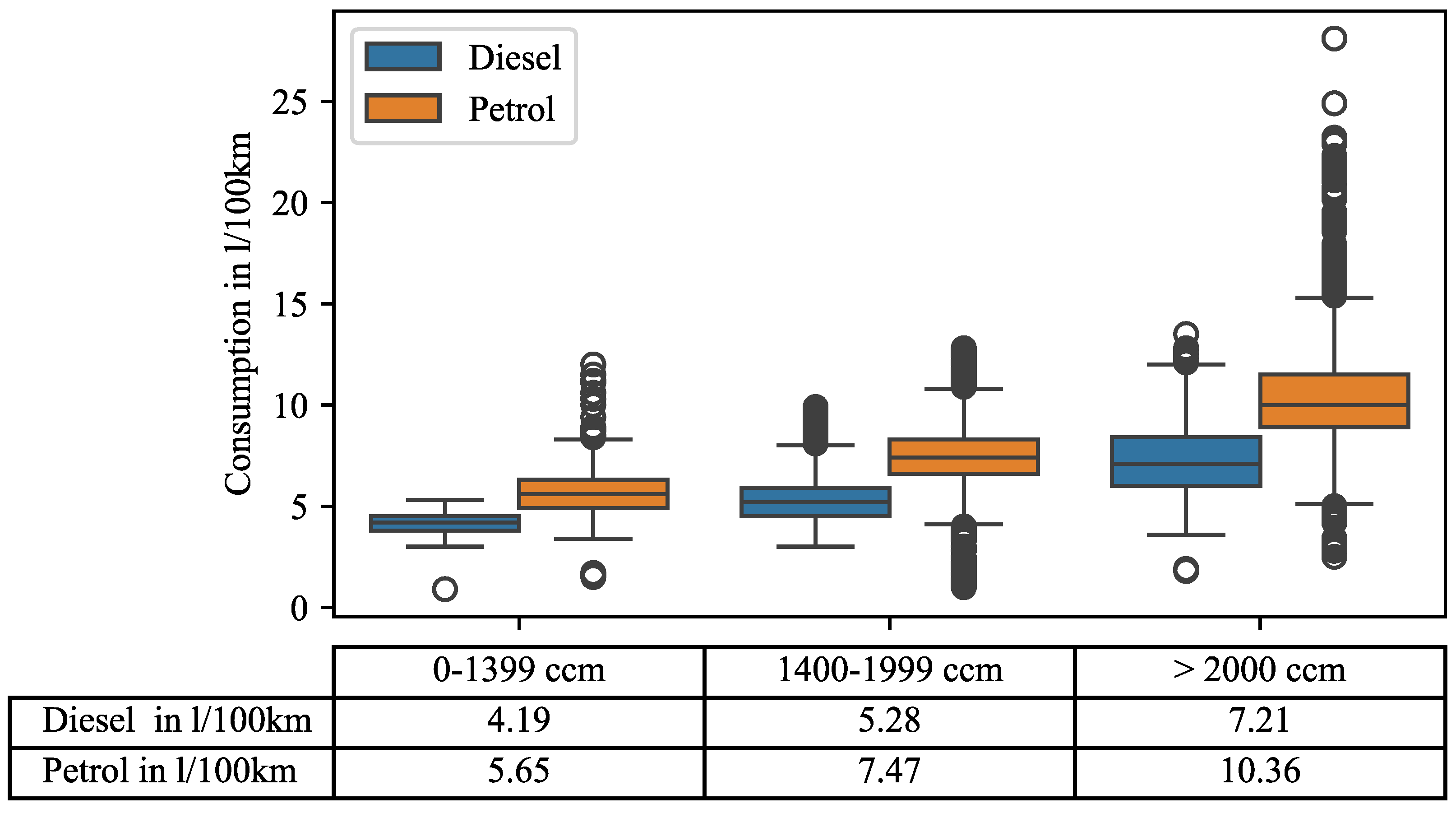
Closing the gaps mentioned above, multiple data sets are used, connected, and analyzed in alignment with three key objectives, as illustrated in Figure 1. Combining vehicle and mobility data with geographical references allows for a novel analysis of road-based emissions. Two different emission calculation methodologies are applied: TtW and WtW. The former assesses emissions generated solely from vehicle operation, while the latter includes emissions caused by preprocesses such as fuel and electricity production. A spatial investigation is conducted using geographical data, allowing for a comparison of the two logics mentioned and for the heterogeneity of input parameters, answering the first and second research questions identified. Additionally, an allocation algorithm for an optimized distribution of BEV is applied to the dataset, which allows the investigation of potentially regionalized political BEV incentives.

2.1. Vehicle Data

To estimate regional differences in GHG emissions, knowledge related to the consumption of the individual vehicle type and the regional distributions of vehicle types is necessary. The Federal Motor Transport Authority (KBA) provides publicly accessible data regarding generic vehicle information such as fuel type and cubic capacity and the areas of their registrations. However, the consumption of the registered vehicles is missing within this data source. Therefore, this data source is combined with a database created by accessing the General German Automobile Club (ADAC) Vehicle Catalog, which contains detailed information, e.g., fuel consumption, on all vehicles in stock in Germany. Within the merging of the data sources, all vehicles are hierarchically clustered into diesel and petrol-powered cars and their respective cubic capacity [39]. The average consumption of all vehicles from 2007 to 2017, respecting the average age of vehicles in stock in the year 2017 [40], are plotted within these clusters and are shown in Figure 2. For all vehicles within that timespan, data regarding the cubic capacity classes and consumption were found in the database. Vehicles lacking assigned cubic capacity class and fuel type were excluded from the analysis. The corresponding fleet was set to the sum of known vehicles. For the years 2017 to 2024 on average, 98.6% regarding cubic capacity classes and 99.2% regarding fuel type were covered compared to the overall fleet size. The box plots illustrate the distribution of consumption values, given in l/100 km, for each fuel type and cubic capacity cluster. The underlying tables state the arithmetic mean for each sample, whiskers are at the 25% and75% percentile, and overlaying circles indicate data outliers. In general, the differences between petrol and diesel-fueled cars are notable, showing higher consumption values for petrol cars by 34% to 44% compared to diesel cars. Moreover, the surplus in consumption rises faster for petrol cars. The resulting arithmetic mean in average consumption is combined with the clusters’ regional distribution for the subsequent analysis.

2.2. Mobility Data

In addition to the energy consumption values of the investigated fleet, mileage and, in particular, its distribution are needed to analyze the regional GHG emissions. The raw data package B2 regional-data package of the Mobility in Germany (MiD) dataset is used to investigate mileage data. The MiD dataset covers $\mathrm{156,420}$ households, $\mathrm{316,361}$ persons, and $\mathrm{960,619}$ trips. While households and persons hold socio-economic and demographic data, the trip data are enriched by, e.g., modes of transport, way distances, and the reason for mobility (work, leisure, etc.) [30]. Using unique identifiers, ways are allocated to persons and their households to gather geographical information. Of all recorded trips, $\mathrm{399,496}$ were recorded as ways traveled by car as a driver and $\mathrm{119,457}$ as a passenger. Trips by foot and by bike play a significant role, accounting for $\mathrm{186,673}$ and $\mathrm{103,833}$ records, respectively. With $\mathrm{73,050}$, public transport is less recorded; other ways such as trucks, motorcycles, cabs, and long-range public transport account for less than $\mathrm{10,000}$ records each. A small area estimation was conducted within the MiD to obtain regional mileage data on the county level. As direct estimations were not possible due to small sample sizes, an indirect approach was performed using the empirical best linear unbiased predictor on the unit level. The resulting dataset provides the overall daily mileage, the number of ways, as well as the modal split for each county in Germany [41].

By combining the passenger car share $s_p$ with the average distance traveled per day, $d_d$, the annual mileage per county r can be derived, as shown in Equation (1):

$$mileag{e}_r=s_p·d_d·365$$

(1)

An analysis of transportation mode shares in Germany reveals a strong dependence on MIVs, both as drivers and passengers, which dominate in terms of both the number of trips (share of ways) and distance traveled (share of kilometers). Across the counties, data show high variation aggregated from counties across Germany, highlighting that MIV drivers account for the most significant proportion of trips and cover the longest distance, underscoring a cultural reliance on private cars, as shown in Figure 3. MIV passengers, though less frequent, still contribute meaningfully to total kilometers, suggesting limited but notable carpooling. In contrast, walking and biking play a significant role in short-distance trips (high share of ways but low share of kilometers). At the same time, public transport has a moderate share of both metrics, indicating it is often used for longer commutes.

2.3. Geographical Data

Geographical data on the municipality level are selected as the initial framework for conducting an in-depth spatial emission analysis. This granular level of geographic information allows for more precise regional comparisons, which is critical for understanding emission variations across different areas. The primary dataset is the ’Communes, 2016—Administrative Units—Dataset’, obtained from GISCO (Geographic Information System of the Commission) by EUROSTAT [42]. This dataset is compiled according to the Nomenclature of Territorial Units for Statistics (NUTS) regulation, standardizing territorial units within the EU, enabling the seamless integration and mapping of auxiliary and geographic datasets. The NUTS logic, deciding certain regional areas, is illustrated in Figure 4. The standardized regional codes provided in this dataset ensure the unique identification of each geographical unit, removing the need for name-based matching and enhancing the reliability of spatial analyses.

Municipal-level data offer insights into local emissions characteristics that are often not visible at higher aggregation levels, being more sparse and potentially incompatible. Therefore, the geographic polygons were aggregated into county units to utilize these local characteristics due to the lack of municipality-specific data, such as fleet composition and mileage. The county level is comparable to Level 3 of the NUTS logic. This aggregation is essential to construct a harmonized dataset that integrates vehicle emissions data derived from fleet stock and mileage data in order to find the sweet spot between regional details and data reliability. Consequently, this combined dataset enables a more comprehensive view of emissions by regions, where data on vehicle usage patterns and emissions estimates can be analyzed together with geographic boundaries, allowing for the identification of high-emission areas and, thus, targeted policy implications.

Using the NUTS-compliant dataset as an anchor, emissions data from vehicle stock and mileage estimates can be consistently matched to geographical areas. This method helps visualize emission distributions across regions and allows the quantification of differentiation in emissions across the various administrative levels.

2.4. Emission Calculation

This work uses a simplified calculation scheme to calculate road-based emissions. Production and recycling emissions are not considered, as this study focuses on the utilization of cars. The use phase relies on energy consumption regarding different fuel types; auxiliary materials such as engine oil, tires, replacement, and general maintenance are excluded, as they are assumed to have a negligible impact on the overall results. First, the average consumption for each region is estimated by splitting the sample fleet into tuple groups of cubic capacity and fuel type. The three subclasses assume the same distribution for petrol and diesel. Each subgroup is assigned a consumption value respecting cubic capacity and fuel type according to Section 2.1. Depending on the fuel type, emission factors are multiplied by the consumption value by fuel type to obtain the emission values shown in Table 1.

In this step, fossil fuels are converted from l to kWh. Depending on the perspective, TtW or WtW values are assigned, whereas TtW only covers emissions directly caused locally, such as burning fuel while driving. As electric vehicles do not emit GHGs locally, their value is usually set to 0. WtW emissions also consider emissions in the chain processes for the production of the corresponding energy source, e.g., refining processes for fossil fuels or electricity production in power plants. Addressing only emissions before actual usage, this represents the well-to-tank (WtT) perspective. Even though this paper states the importance of using WtW values to calculate emissions, TtW values are also given for comparability.

Given the average mileage ${\overline{M}}_r$ for each region r (see Section 2.2), the number of registered passenger cars $c_{ft,cc,r}$ by fuel type $ft$ together with (if the fuel type is either petrol or diesel) the cubic capacity $cc$ for each region, and the average consumption values stated in Figure 2, the emission per kilometer driven for each region is calculated as follows:

$${\overline{\mathrm{Emission}}}_r=\sum _f{\mathrm{share}}_{f,r}·\left(\sum _s{\mathrm{share}}_{s,r}·{\mathrm{consumption}}_{f,s}\right)·e_{f,x},$$

(2)

where x is either TtW or WţW, depending on the perspective.

The values for the consumption are obtained as described in Section 2.1 combined with the emission factors for each fuel type as shown in Table 1. Compared to other sources such as [43], reporting $2.83$ $\mathrm{k}$$\mathrm{g}$CO_2-eq. for petrol and $3.18$ $\mathrm{k}$$\mathrm{g}$CO_2-eq. for diesel, the calculated values are in comparable dimensions and will be used for the further analysis.

Table 1. Emission factors for petrol, diesel, and electricity regarding TtW, WtT, and WtW in $\mathrm{k}$$\mathrm{g}$CO_2-eq./kWh.

	Petrol	Diesel	Electricity	Source
in $\mathrm{k}$$\mathrm{g}$ CO2-eq./l
TtW	2.60	2.95	-	[44,45]
WtT	0.14	0.13	-	[46,47]
WtW	2.73	3.08	-	[48]
in $\mathrm{k}$$\mathrm{g}$ CO2-eq./kWh
TtW	0.297	0.296	0	[44,45]
WtT	0.016	0.013	0.552	[46,47,49]
WtW	0.312	0.309	0.552	[48]

Energy content for petrol and diesel are assumed to be $8.76$ and $9.96$ kWh/l. Note: WtT values for petrol and diesel refer to 2020.

Table 1. Emission factors for petrol, diesel, and electricity regarding TtW, WtT, and WtW in $\mathrm{k}$$\mathrm{g}$CO_2-eq./kWh.

	Petrol	Diesel	Electricity	Source
in $\mathrm{k}$$\mathrm{g}$ CO2-eq./l
TtW	2.60	2.95	-	[44,45]
WtT	0.14	0.13	-	[46,47]
WtW	2.73	3.08	-	[48]
in $\mathrm{k}$$\mathrm{g}$ CO2-eq./kWh
TtW	0.297	0.296	0	[44,45]
WtT	0.016	0.013	0.552	[46,47,49]
WtW	0.312	0.309	0.552	[48]

Energy content for petrol and diesel are assumed to be $8.76$ and $9.96$ kWh/l. Note: WtT values for petrol and diesel refer to 2020.

To obtain total emissions for each region r, mileage values and consumption values are combined, assuming the same mileage for each car in the area of interest as shown in Equation (3).

$$\begin{array}{cc}\hfill \mathrm{Total}{\mathrm{Emission}}_r& ={\mathrm{mileage}}_r·\sum _f{\mathrm{share}}_{f,r}·\left(\sum _s{\mathrm{share}}_{s,r}·{\mathrm{consumption}}_{f,s}\right)·e_{f,x}\hfill \\ \hfill & ={\mathrm{mileage}}_r·{\overline{\mathrm{emission}}}_r\hfill \end{array}$$

(3)

This, finally, allows us to obtain the total emission for all regions with Equation (4):

$$\begin{array}{cc}\hfill \mathrm{Total}\mathrm{Emission}& =\sum _r{\mathrm{mileage}}_r·\sum _f{\mathrm{share}}_{f,r}·\left(\sum _s{\mathrm{share}}_{s,r}·{\mathrm{consumption}}_{f,s}\right)·e_{f,x}\hfill \\ \hfill & =\sum _r{\mathrm{mileage}}_r·{\overline{\mathrm{emission}}}_r\hfill \\ \hfill & =\prod _{r,f,s}\left({\mathrm{mileage}}_r·{\mathrm{share}}_{f,r}·{\mathrm{share}}_{s,r}·{\mathrm{consumption}}_{f,s}·e_{f,x}\right)\hfill \end{array}$$

(4)

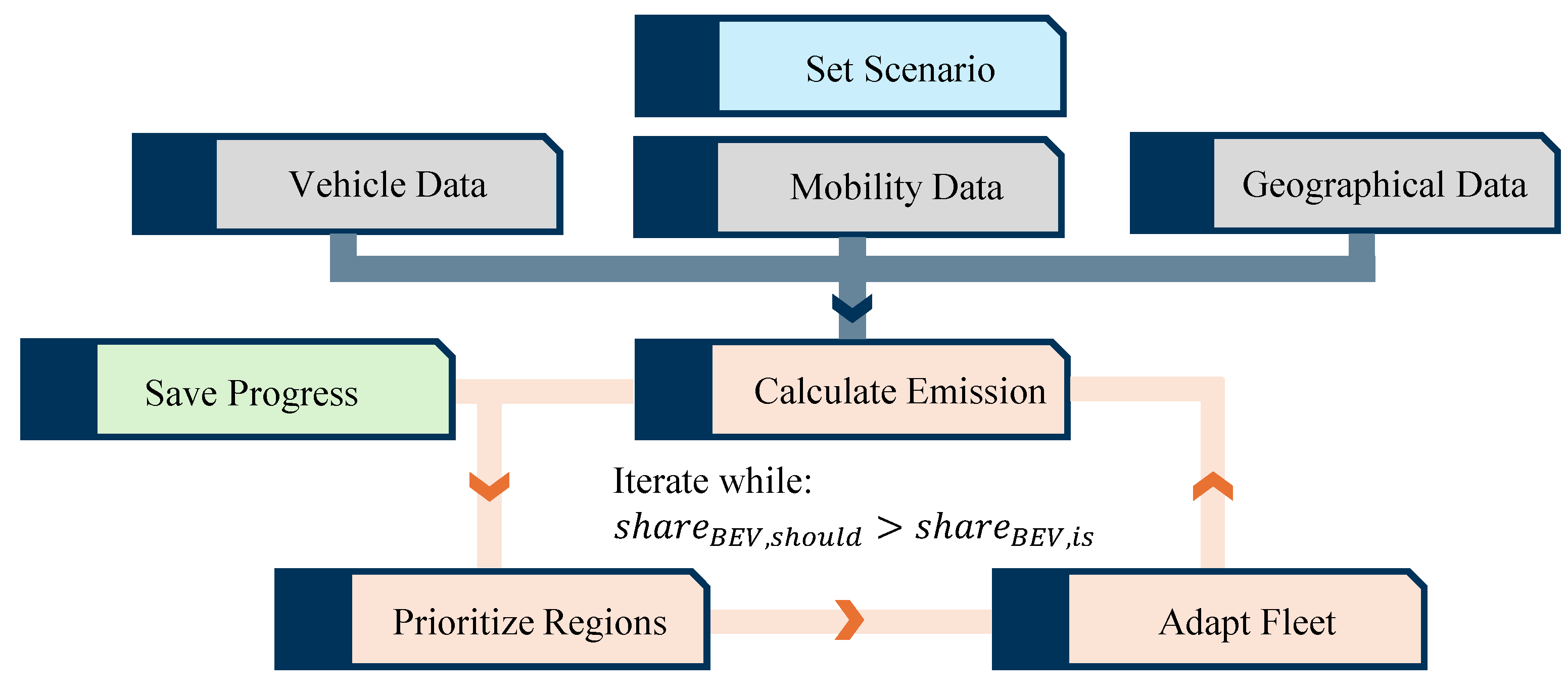
2.5. Allocation Algorithm

Last, to illustrate the example of using an increase of the BEV share in the fleet as one possible approach to reduce GHG emissions, it is of interest to evaluate the potential of using regionalized data to optimize the distribution of such vehicles. A three-step approach is used, as shown in Figure 5.

First, a scenario is defined with a target share of BEVs in the overall fleet and a batch size, determining the number of conventional vehicles replaced in each iteration. The amount of iterations is defined by the ratio of vehicles to add to the fleet over the chosen batch size rounded to the next integer value, while the amount of vehicle to add is determined by the current and target share of BEVs. Next, vehicle, mobility, and geographical data are loaded according to Section 2.1, Section 2.2 and Section 2.3. Before any adaptions, the current consumption values and emissions are calculated for each county, as shown in Section 2.4. Before the change of the fleet composition, the county with the highest WtW emissions is selected, which is reevaluated in each iteration, as shown in Equation (5). The corresponding fleet is adapted by replacing one batch of conventional cars with BEVs. The corresponding region’s current share of petrol- and diesel-powered cars determines the share of replaced conventional vehicles.

$$\begin{array}{cc}\hfill r^{*}& =sup\left\{r\mid {\mathrm{Impact}}_r\right\}\hfill \\ \hfill \mathrm{where}{\mathrm{Impact}}_r& ={\mathrm{mileage}}_r·{\overline{\mathrm{Emission}}}_r\hfill \end{array}$$

(5)

The batch size is set to be a multiple of 401, corresponding to the number of counties in Germany in the year 2017 [50]. With this, the allocation on the national level was simplified by allocating one BEV per batch multiple to each county. This approach represents a non-directed distribution across the whole nation. With higher batch multiplicators, the algorithm performance can be optimized while the increase in inaccuracy stays low. At the last iteration, the delta between the desired amount of electric vehicles and the current amount is calculated, and the batch size is corrected to avoid overshooting.

3. Results

This section is divided according to the three main contributions stated in Section 1.1. It provides a concise description of the results, first of the spatial distribution of consumption and mileage data. Next, the difference between TtW and WtW perspectives is illustrated. Lastly, following the allocation algorithm, the beneficial effect of respecting the geographical distribution is shown.

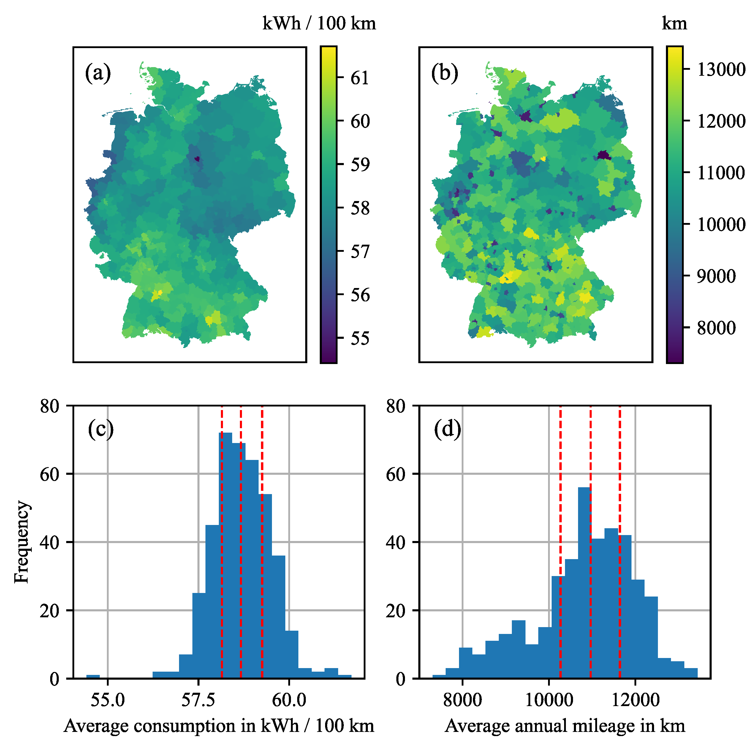
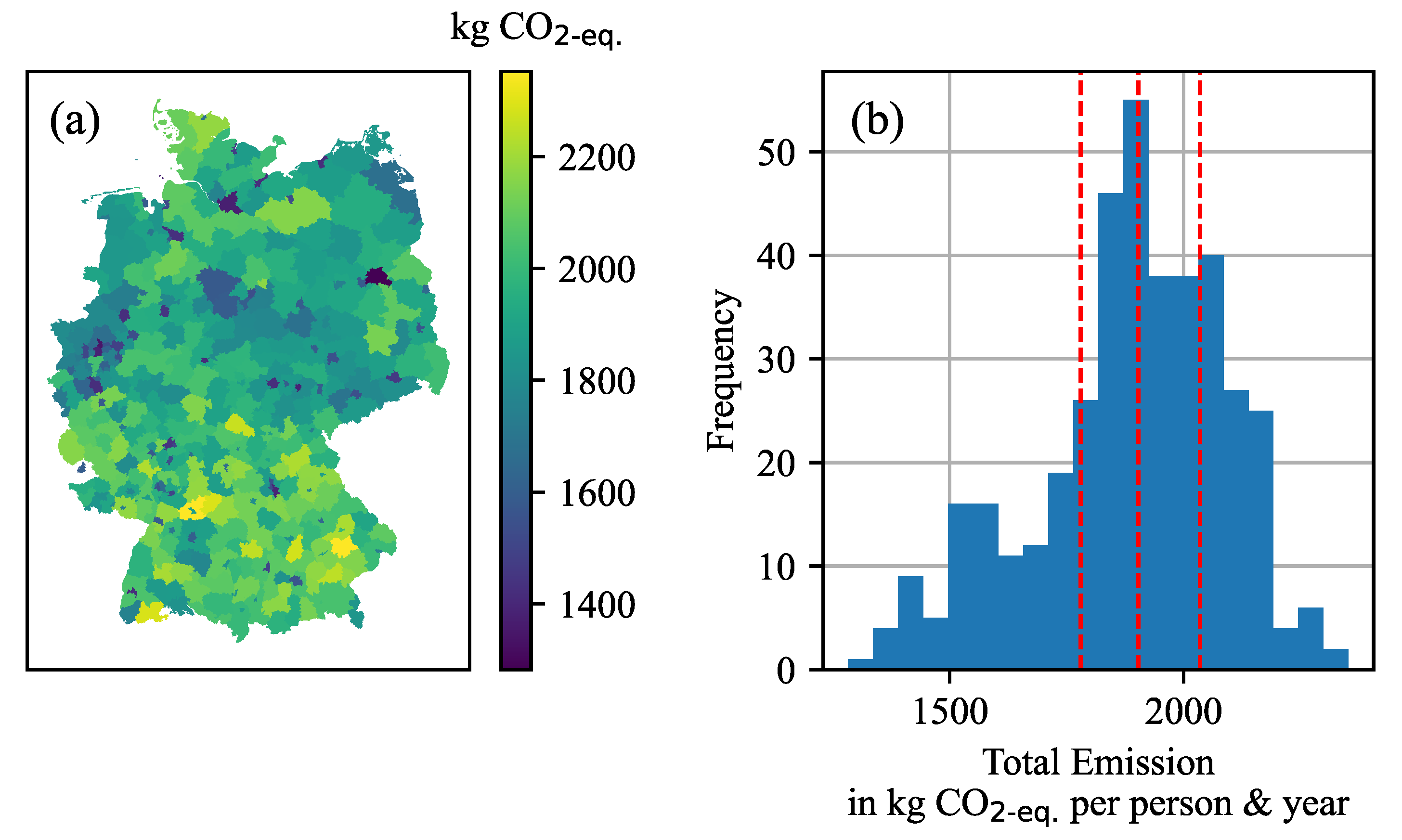
3.1. Heterogeneity of Consumption, Mileage, and Emissions

Figure 6 reveals spatial disparities in both average consumption (subplots a and c) and annual mileage patterns (subplots b and d). The spatial analysis indicates that the average vehicle consumption of fuel-powered vehicles (measured in kWh/100 km) varies significantly across regions. Southern regions such as Bavaria and Baden-Württemberg show higher consumption values than northern and eastern areas led by Stuttgart, Starnberg, Baden-Baden, Böblingen, and Munich with consumption values from 60.76 kWh/100 km to 61.71 kWh/100 km. The northwestern area, which borders the Netherlands, and the area of Wolfsburg show low consumption values. Wolfsburg itself shows the lowest value, which is followed by the counties of Bentheim, Kleve, and Heinsberg, ranging from 54.4 kWh/100 km to 56.8 kWh/100 km. In general, the mean of this distribution is $58.70$ with a standard deviation of $0.814$. The histogram shows a close to symmetrical appearance with a skew of $-0.070$.

Regarding the mileage distribution, the heterogeneity is more obvious, while other trends are revealed. Statistically speaking, the values are within the range of 7308 km to 13,435 km, with the mean at $\mathrm{10,833}$, and the standard deviation of $1161.8$. Urban areas generally report lower annual mileage, which is likely due to shorter travel distances and better public transport infrastructure, whereas rural regions show higher averages. The county of Wolfsburg shows the highest mileage value with $13.435$ km/a driven by car, which was followed by Heilbronn, Dingolfing-Landau, and Rhön-Grabfeld. The least kilometers traveled by car are found in Nuremberg, Hamburg, Gelsenkirchen, and Berlin, ranging from 7308 km to 7862 km. With a skewness of $-0.5966$, this distribution is comparable to the consumption values, which show a light negative skew but are comparable to normal distribution. Combining both inputs allows for a simplified emission calculation. Figure 7 draws a comparable picture as Figure 6b. As mileage data are, on the one hand, higher in magnitude and, on the other, higher in variance (showing a spread of $\pm 32.5\%$ vs. $\pm 7.3\%$), this behavior appears compelling. Regarding general statistical properties, this distribution shows a mean of 1886, a standard deviation of $204.5$, a skew of $-0.519$, and a spread of $\pm 32.0\%$. In general, southern counties show higher values with rural areas showing higher values than urban areas. Similar to the mileage data, the county Heilbronn leads regarding emissions of $2352.2$ $\mathrm{k}$$\mathrm{g}$CO_2-eq./person and year, which is followed by Dingolfing-Landau, Hohenlohekreis, and Waldshut. The last places are Berlin, Gelsenkirchen, Hamburg, and Essen with values from 1282.5 $\mathrm{k}$$\mathrm{g}$CO_2-eq./person and year to 1384.2 $\mathrm{k}$$\mathrm{g}$CO_2-eq./person and year.

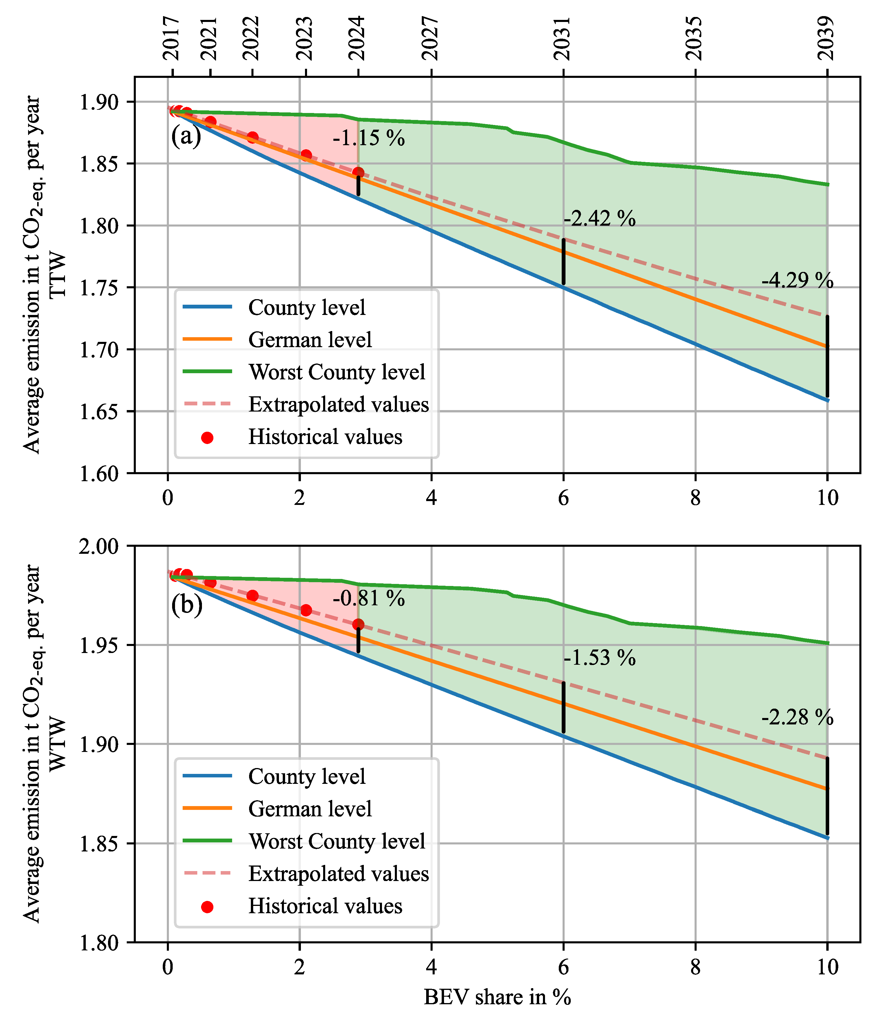
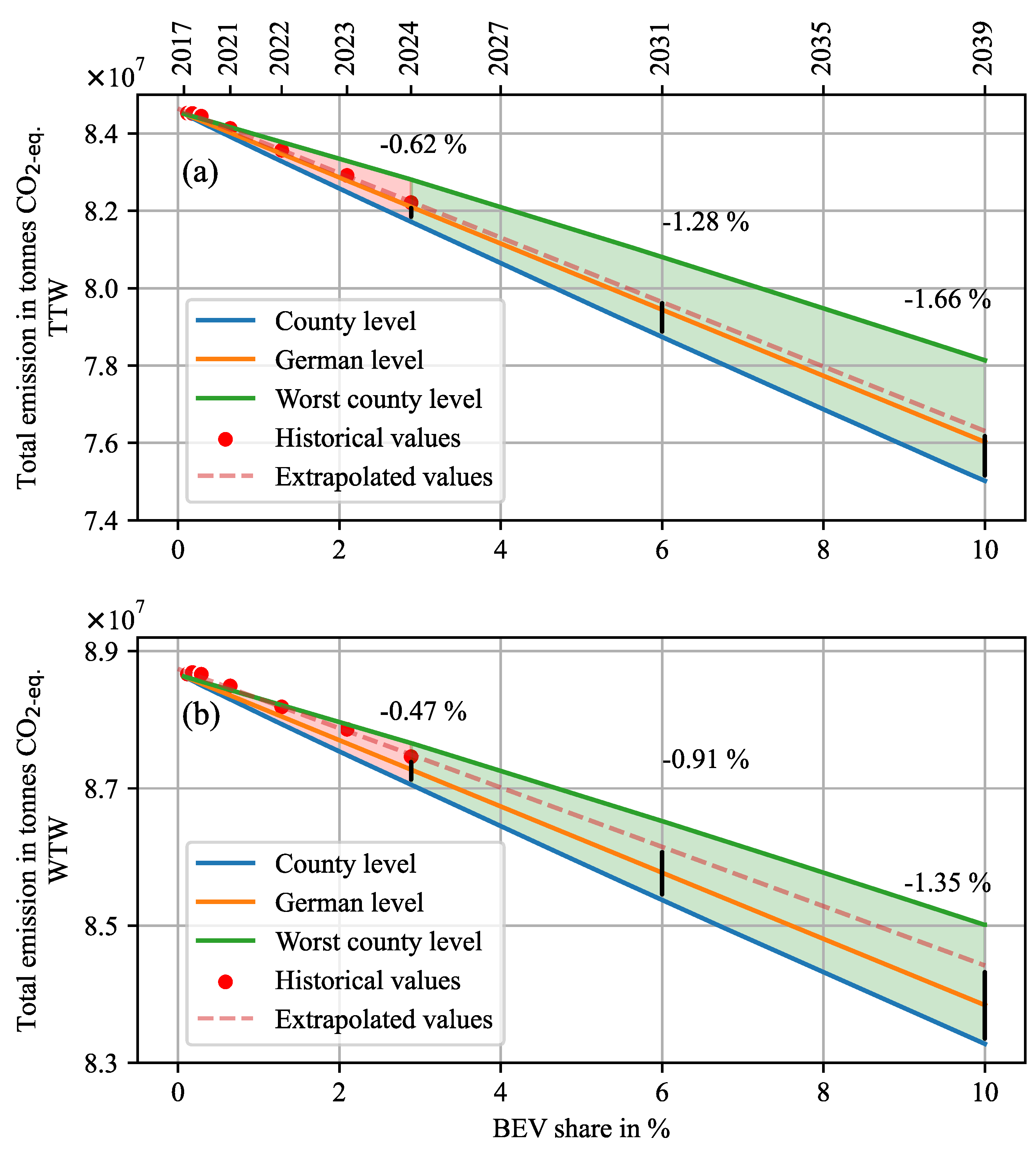
3.2. TtW vs. WtW Perspectives

Depending on the logic and perspective of the analysis, a TtW or WtW approach is used. The disparity between both is often neglected. Nevertheless, a difference in magnitude and in its distribution can be observed. Using both perspectives, Figure 8 reveals these differences. Using a TtW approach, emissions that occur while producing and distributing the energy carrier used in cars are usually neglected. Respecting such upstream processes changes the average emission per kilometer measured in CO_2-eq.. On the one hand, fossil fuel cars now take refinery processes into account; on the other hand, now, BEVs emit GHGs due to the production of electricity necessary for driving. For the year 2017, the mean TtW emission is around $17.4$ $\mathrm{k}$$\mathrm{g}$CO_2-eq./100 km, and WtW is around $18.2$. Figure 8b,c show the effect of a surplus of BEVs in the fleet, increasing their share to 10% and 30% while holding all other parameters constant.

With an increased BEVs share, three characteristic changes can be observed. First, the average consumption values for both TtW and WtW decrease to $16.01$ and $17.6$ $\mathrm{k}$$\mathrm{g}$CO_2-eq./100 km, and $12.5$ and $15.6$ $\mathrm{k}$$\mathrm{g}$CO_2-eq./100 km for adapted fleets with $10\%$ and 30% shares of BEVs. This is due to higher shares of BEVs, and the reduction is a logical consequence, as they are more energy-efficient than conventional cars. Second, the gap between TtW and WtW average values increases with higher BEV shares. As the differences in the TtW and WtW emission factors are smaller for fossil-fueled cars than for BEVs, the rise in such causes higher deviations in the mean values. This effect is correlated to the share of BEVs, which can be observed by comparing the subplots in Figure 8. Last, the distribution spread increases with higher BEVs shares. TtW emissions show a rise in their standard deviation from $0.25$ in 2017, over $0.45$ for the 10% scenario, and $1.0$ for the 30% scenario. Similarly, WtW’s standard deviation increases from $0.24$, over $0.82$, up to $1.87$, respectively. Possibly, this effect can be caused by the calculation logic, increasing the overall share to higher rates by using appropriate multiplicators. Counties with already relatively high BEV shares will show higher increases in their own electrification than others while all together averaging on the target share value.

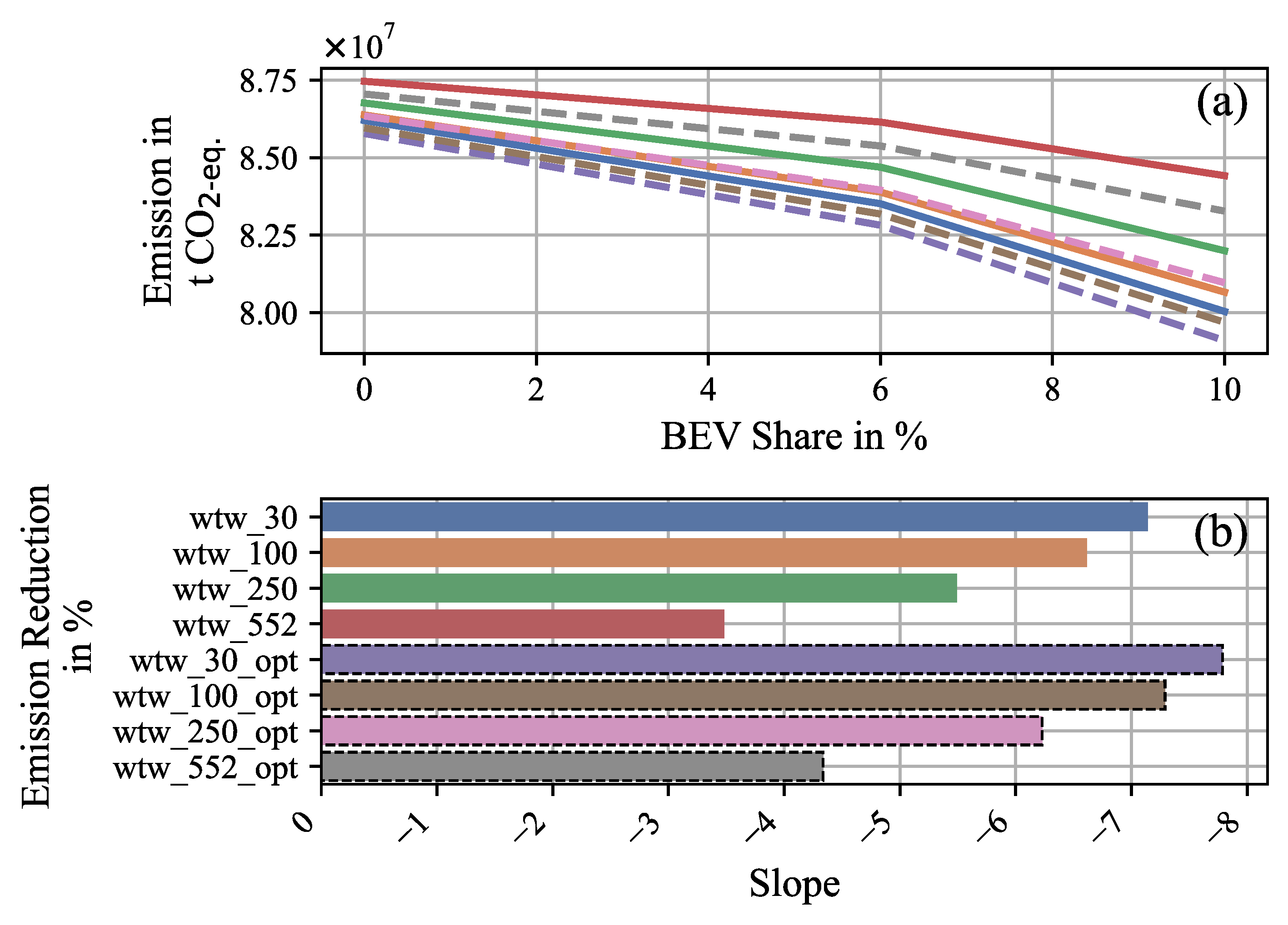
3.3. Spatially Informed BEV Distribution

To show the effect of taking regional factors into account, the share of electric vehicles in the fleet was increased stepwise, and the reduction behaviors with respect to the average emissions per year and total emissions were investigated. Every analysis starts with the fleet situation from 2017. With a surplus of BEVs in the fleet, emissions can be reduced; however, different effectiveness can be observed in different distribution strategies. Three different strategies were investigated: county refers to an optimal distribution aiming to minimize the emissions in every step; bad county tries to do the opposite, adapting fleets in regions where the least benefit is expected; german distributes new BEVs to every county at the same time, which are weighted by the number of vehicles in each county. Historical information is added to the analysis. This stems from the annual fleet reports from the KBA by county. With this, the changed fleet composition is transferred to the data, annual mileage, and the distribution of cubic classes over counties, which were kept unchanged, as the fleet composition by fuel type is the major objective of this study. For this analysis, a target share of 10% was used with a batch size of 400 vehicles, which was distributed in each of the 11.351 iterations.

Figure 9 shows the reduction in the average emission per car per year, which was given in $\mathrm{t}$ CO_2-eq.. For this, the values were calculated for each county in Germany initially and for every iteration until the target share was reached. The results show that an increased share of BEVs will always lead to a reduction in the specific emission independent of the calculation perspective regarding TtW and WtW. If BEVs were distributed optionally, a surplus of 1.15% or 0.81% in the reduction by 2024 could have been achieved. Extrapolating the historic values allows for an extrapolation of this potential, reaching 4.29% or 2.28%. The average emission for a German passenger car per year for 2017 lies around $1.89$ $\mathrm{t}$CO_2-eq. or $1.98$ $\mathrm{t}$CO_2-eq., dropping to $1.84$ $\mathrm{t}$CO_2-eq. or $1.96$ $\mathrm{t}$CO_2-eq. in the year 2024 according to the historic values. The WtW emissions can decrease by 6.6% when reaching a 10% share, while TtW emissions can be reduced by 12.2%. This behavior can be explained by the different calculation schemes explained in Section 3.2. Moreover, this explains the higher delta visible in the TtW perspective (subplot a). The years displayed on the upper x-axis correspond to the penetration rate extrapolated using the historical values. As penetration rates might vary in the real world, the lower x-axis, displaying the BEV share in percentage, is only linked to the years for the red dashed line.

Similar to the results regarding the average emissions, the same analysis was conducted to investigate the reduction potential for the overall road-based passenger car emissions. To obtain these, the average emission values, whose mean values can be seen in Figure 10, are multiplied and summed with the regional annual mileage values.

Both results show the reduction potential by implementing BEVs into the fleet while reducing conventional passenger cars. Using a smart distribution of these vehicles, a surplus can be achieved. This depends on two general circumstances. First, there is the average consumption given by the share between different fuel types and the composition by cubic capacity used as a proxy to include more and less efficient cars. As shown in Section 2.1, this has a significant impact on the consumption of the cars. Second, the annual mileage also has a significant impact. Section 2.2 reveals the heterogeneity of these data, supporting the hypothesis of its influence on road-based emissions. Last, whether the TtW or the WtW perspective is used for the calculation, different absolute values, decay rates, and deltas between the strategies are observed for both specific annual emissions for a single representative car and the overall emissions. Regarding the regional analysis, it can be observed in which counties changes were made more often than in others. Using the county approach, the algorithm has addressed 276 of 400 counties, whereof the counties of Heilbronn, Rhein-Sieg-Kreis, Karlsruhe, Mettmann, Main-Taunus-Kreis, Märkischer Kreis, and Wolfsburg already account for 10.53% of the changes. Using the bad county approach, cities such as Berlin, Hamburg, and Cologne are top-listed, accounting for more than half of the changes ($52.52$ %). Inspecting the underlying regional data regarding the mentioned counties, the significant influence of the average annual mileage becomes obvious. Examining auxiliary data, the respective population size correlates with the emission-saving potential as well, supporting the thesis that more rural areas show higher potential. It should be noted that these results imply that both variables could jointly contribute to the variation in the saving potential; however, a coupled influence is possible. Another possible interpretation of the observed results is in combination with the national GHG emission targets. By 2030, Germany’s annual emission limits for the transport sectors are set to 82 $\mathrm{M}$$\mathrm{t}$CO_2-eq., of which around 78 $\mathrm{M}$$\mathrm{t}$CO_2-eq. can be attributed to road-based emissions, of which around 48 $\mathrm{M}$$\mathrm{t}$CO_2-eq. passenger cars would account for [2,3,51]. Corrected by the general deviation with respect to reported values, this would conclude in a gap of 43% in the base scenario, which is almost identical to the gap reported by the projection report. Using the regional optimized allocation, this can be reduced by 2% solely by arranging BEVs spatially optimally, while assuming the same mileage and fleet stock values, as well as a static market ramp-up of BEVs, lessens this effect.

4. Discussion

This paper shows the importance of accounting for spatial information when evaluating road-based emissions. It analyzes the potential of additional emission reduction when using them, allowing for a deeper understanding and valuable information to shape measures more efficiently. Further, the difference between the TtW and the WtW perspective is highlighted.

The first key result shows that the underlying data regarding vehicle distribution and mileage vary significantly across regions. This variability underscores the importance of granular spatial data when analyzing emissions. National averages tend to mask these regional differences, leading to suboptimal policy recommendations. This finding emphasizes the need for localized policymaking approaches that are tailored to each region’s unique characteristics. However, the data used refer to 2017. As more recent mobility data are unavailable now, vehicle data regarding 2017 were used to ensure data matching. As mobility behavior, in this case, annual passenger car mileage values and their distribution, have a considerable impact, the data availability limits the findings. Another issue encountered during this study is the changing regional boundaries, as counties can change names, unite, or separate. This is an unforeseen challenge when trying to automize analysis over several years, and it needs time-intensive manual preprocessing. Further, the vehicle data used in this study do not differentiate between private and company vehicles. However, it is known that the type of vehicle and their consumption values differ against the average, especially for hybrid vehicles [52]. Further, the availability of company cars appears to have a significant impact on the number of cars per household and the share of ICE cars [53]. Lastly, the regional mileage values are assumed to be equal across all covered fuel types, which does not hold true necessarily, as BEVs tend to drive lower distances than conventional cars [54].

The second key result shows the differences between both perspectives, TtW and WtW, when calculating emission values. Regarding fuels, the emission values are almost constant over the years, as the resulting emissions from burning fuel are defined by their chemical structure. The WtT emissions are determined by the refinery processes and transportation, whose change over the years is negligibly low. The grid mix used for accounting for the WtW emission for BEVs shows high sensitivity in such studies [55,56]. For the reference year 2017, the emission value of $0.552$ was used. However, this value is assumed to reach $0.498$ in 2022 [49]. This decrease would narrow the gap visible in Section 3.2 and further benefit the introduction of electric vehicles in the fleet. With this, the decrease in overall emissions is steeper, increasing the potential gap regarding the different allocation strategies. Scaled by the number of kilometers traveled, the importance of the underlying emission factors is further stressed as it is one of the main drivers regarding the overall emissions [55].

The third key result illustrates a case where different strategies are applied to assign BEVs and replace conventional cars. For the specific emissions, the potential of optimized assignment reaches 4.29% for TtW and 2.28% for WtW. These values are smaller for total emissions, ranging around 1.5%. As the potential takes the linear extrapolated line based on the historical values as a reference, this underlies uncertainties, as it is unknown whether this linear behavior matches future effects. This would result in a change of the year’s annotations on top of the graphs but does not influence the curves’ shape. As mentioned above, the emission factor for electricity plays a major role and can lead to significant deviations in the results. Figure 11a illustrate the reduction curves between up to 10%, for scenarios covering electricity emission values from 552 $\mathrm{g}$CO_2-eq./kWh down to 30 $\mathrm{g}$CO_2-eq./kWh, passing through 100 $\mathrm{g}$CO_2-eq./kWh and 250 $\mathrm{g}$CO_2-eq./kWh, where $opt$ represents the regional optimized strategy, and the others represent extrapolated historical values. In general, with lower WtW emissions for electricity, the overall emission saving is higher, and the slope of the curves increases, as seen in subplot (b). This leads to a faster reduction in GHG emissions. However, the difference between the optimized against the baseline curve decreases with lower emission values, indicating higher potential if emissions from electricity production remain high. As the emission factor for electricity decreases, the gap between TtW and WtW will decrease. Further, with a lower emission factor, the potential benefit decreases. The average German grid mix was used for this study, neglecting the effect of solar-powered home charging. Moreover, the change in driving behavior was neglected using the annual mileage values from 2017. As they were also used to calculate the values for the years from 2018 to 2024, a deviation of these values is expected. The annual mileage for cars, on average, has seen a decrease from 13,931 km/year in 2017 to 12,320 km/year in 2023 or 11.6% [57]. As for this study, different mileage values by fuel type are not considered, as a change in the mileage values will only lead to a change in the magnitude of GHG emission but not in the percentual benefit. In future work, this should be addressed, and if possible, more recent data should be used. Further, the values can be specified using fleet age composition, cubic capacity, and fuel type as input variables for a more detailed mileage estimation. This could be another approach that challenges the values from the MiD study in future research. Although deviations are expected to influence the values presented in this study, political incentives—such as subsidies for electric vehicle purchases—can enhance their efficiency by utilizing regional data to more precisely support the ramp-up of BEVs to areas where their benefits are maximized.

While a novel approach to analyzing regional informed emissions, we need to underline the mentioned assumptions and simplifications. With the release of more recent data, especially mobility data such as the MiD study, both the current status should be analyzed and put into context with auxiliary information such as introduced or dropped policies, new regulations, and other external influencing factors. Apart from investigating the use phase of vehicles, a more holistic perspective can be achieved by performing comparative life cycle assessments. Even facing limitations, this study shows the importance of regionalized adaptions to the fleet. For this, the findings of the spatial heterogeneity of vehicle stock and mobility data can be utilized, as well as the regionally different reduction potential, by introducing BEVs to the fleet, also with supposedly outdated data already today. This can be achieved by designing spatial sensitive incentives such as subsidies for BEVs with respect to a regional factor. Areas where the introduction of BEVs would show higher potential to reduce GHG emissions are favorable and can be addressed with higher subsidies. As rural areas tend to show higher potential in general than urban areas, the support for home charging systems, potentially with coupled PV systems, can be increased as the rate of private homeowners is higher in these regions. At the same time, this does not mean that the ramp-up of, e.g., public charging infrastructure or urban mobility hubs shall be abolished, but rather shifting the focus toward rural Germany. Moreover, this approach has the potential to be applied across other nations, depending on their national goals toward green transportation.

5. Conclusions

This study addresses the benefit of taking regional aspects in Germany into account. Furthermore, the differentiation between both TtW and WtW is shown. With the introduction of locally zero-emission vehicles such as BEVs, the TtW perspective becomes less comprehensive. Lastly, utilizing regional information, the concept of a spatially informed allocation of BEVs is introduced and performed. In general, the data necessary to estimate GHG emissions differ across the counties in Germany. In addition to vehicle stock data, which allows us to investigate the differences by fuel type and cubic capacity classes, annual mileage data differ significantly. These insights alone make it possible to create regional informed measures to tackle the emission gap within the transportation sector by directly addressing areas of high mileage and/or highly emitting ICEs. Values differ depending on the perspective when calculating GHG emissions. Moreover, when introducing more BEVs to the fleet, the deviation between both increases, indicating a less accurate calculation when solely relying on the TtW perspective. For this, it is highly recommended that both approaches be considered to ensure comparability and accuracy in future studies. Finally, an analysis was conducted to illustrate the potential of using the regional distributed data. Regarding average emission values per car, a surplus of 4.29% to 2.28% can be achieved; for the total emissions, this range is 1.66% to 1.35%. These numbers highly rely on the emission factor of electricity. Furthermore, the evolution of mileage values can influence these numbers significantly. Inspecting counties after using the optimized allocation algorithm, rural counties are addressed more often than urban ones. How other factors, such as average household income, existing infrastructure for alternative commuting, and whether an intermediate aggregated regionalization is sufficient, are up for future studies.

The main conclusions of this work are summarized below:

• Underlying data needed to calculate road-based emissions of passenger cars differ significantly across regions. Evaluated for counties in Germany, spreads of $\pm \mathrm{7.3\%}$ and $\pm \mathrm{32.5\%}$ for consumption and annual mileage values data were calculated.
• The choice of perspective has a significant influence on the absolute values. Moreover, the composition of the fleet and respected electricity mix further deviates TtW and WtW values, their gap, and the spread of values.
• Spatially informed calculations and the regionally optimized allocation of BEVs to the fleet can reduce GHG emissions more efficiently than current approaches. Using this approach allows for improved policies incentivizing green transportation, such as subsidies for BEVs, leading to a more efficient use of governmental resources.

References

1. Olhoff, A.; Bataille, C.; Christensen, J.; den Elzen, M.; Fransen, T.; Grant, N.; Blok, K.; Kejun, J.; Soubeyran, E.; Lamb, W.; et al. Emissions Gap Report 2024: No More Hot Air … Please! With a Massive Gap Between Rhetoric and Reality, Countries Draft New Climate Commitments; United Nations Environment Programme: Nairobi, Kenya, 2024. [Google Scholar] [CrossRef]
2. Eurostat. Greenhouse Gas Emissions by Source Sector: Product Code: env_air_gge; European Environment Agency (EEA): Copenhagen, Denmark, 2022. [Google Scholar] [CrossRef]
3. Anteil des Verkehrs an den Treibhausgas-Anteil des Verkehrs an den Treibhausgas-Emissionen in Deutschland. Available online: https://www.umweltbundesamt.de/daten/verkehr/emissionen-des-verkehrs#verkehr-belastet-luft-und-klima-minderungsziele-der-bundesregierung (accessed on 4 December 2024).
4. Kuhnimhof, T.; Wirtz, M.; Manz, W. Decomposing Young Germans’ Altered Car Use Patterns. Transp. Res. Rec. J. Transp. Res. Board 2012, 2320, 64–71. [Google Scholar] [CrossRef]
5. Eisenmann, C.; Nobis, C.; Kolarova, V.; Lenz, B.; Winkler, C. Transport mode use during the COVID-19 lockdown period in Germany: The car became more important, public transport lost ground. Transp. Policy 2021, 103, 60–67. [Google Scholar] [CrossRef]
6. United Nations Framework Convention on Climate Change (UNFCCC). Paris Agreement. Adopted at the 21st Conference of the Parties (COP21), Paris, France. Available online: https://unfccc.int/process-and-meetings/the-paris-agreement/the-paris-agreement (accessed on 11 March 2025).
7. Klimaschutzplan 2050: Klimaschutzpolitische Grundsätze und Ziele der Bundesregierung. Available online: https://www.bmwk.de/Redaktion/DE/Publikationen/Industrie/klimaschutzplan-2050.pdf?__blob=publicationFile&v=1 (accessed on 11 March 2025).
8. Klimaschutzprogramm 2030 der Bundesregierung zur Umsetzung des Klimaschutzplans 2050. Available online: https://www.bundesregierung.de/resource/blob/974430/1679914/e01d6bd855f09bf05cf7498e06d0a3ff/2019-10-09-klima-massnahmen-data.pdf?download=1 (accessed on 11 March 2025).
9. Bundestag. Bundes-Klimaschutzgesetz vom 12. Dezember 2019 (BGBl. I S. 2513), das Durch Artikel 1 des Gesetzes vom 18. August 2021 (BGBl. I S. 3905) geändert Worden Ist: KSG. Available online: https://www.gesetze-im-internet.de/ksg/KSG.pdf (accessed on 26 February 2024).
10. Bundestag. Erstes Gesetz zur Änderung des Bundes-Klimaschutzgesetzes. Available online: https://www.bgbl.de/xaver/bgbl/start.xav?startbk=Bundesanzeiger_BGBl&start=//*%5b@attr_id=%27bgbl121s3905.pdf%27%5d#__bgbl__%2F%2F*%5B%40attr_id%3D%27bgbl121s3905.pdf%27%5D__1708944546162 (accessed on 26 February 2024).
11. Bundestag. Zweites Gesetz zur Änderung des Bundes-Klimaschutzgesetzes. Available online: https://www.recht.bund.de/bgbl/1/2024/235/regelungstext.pdf?__blob=publicationFile&v=2 (accessed on 11 March 2025).
12. Projektionsbericht 2023 für Deutschland. Available online: https://www.umweltbundesamt.de/sites/default/files/medien/11850/publikationen/39_2023_cc_projektionsbericht_12_23.pdf (accessed on 8 February 2024).
13. Overview of EPA’s MOtor Vehicle Emission Simulator (MOVES5). Available online: https://www.epa.gov/system/files/documents/2024-11/420r24011.pdf (accessed on 5 December 2024).
14. Ntziachristos, L.; Gzatzoflias, D.; Kouridis, C.; Samaras, Z. COPERT: A European Road Transport Emission Inventory Model. In Environmental Science and Engineering; Springer: Berlin/Heidelberg, Germany, 2009; pp. 491–504. [Google Scholar] [CrossRef]
15. Allekotte, M.; Biemann, K.; Heidt, C.; Colson, M.; Knörr, W. Aktualisierung der Modelle TREMOD/TREMOD-MM für die Emissionsberichterstattung 2020 (Berichtsperiode 1990–2018): Berichtsteil “TREMOD”. Available online: https://www.umweltbundesamt.de/sites/default/files/medien/1410/publikationen/2020-06-29_texte_116-2020_tremod_2019_0.pdf (accessed on 16 February 2024).
16. Bergk, F.; Heidt, C.; Knörr, W.; Keller, M. Erweiterung der Software TREMOD um Zukünftige Fahrzeugkonzepte, Antriebe und Kraftstoffe; Vol. Heft 113, Berichte der Bundesanstalt für Straßenwesen; Fachverlag NW in der Carl Schünemann Verlag GmbH: Bremen, Germany, 2016. [Google Scholar]
17. Schmidt, M.; Höpfner, U. 20 Jahre ifeu-Institut; Vieweg+Teubner Verlag: Wiesbaden, Germany, 1998. [Google Scholar] [CrossRef]
18. Allekotte, M.; Heidt, C.; Knörr, W.; Kotzagiorgis, S.; Schneider, W. Modellintegration des TransportVisualisierungsmodells (TraViMo) und dem Transport Emission Model (TREMOD). Available online: https://digital.bibliothek.uni-halle.de/pe/download/pdf/3252971?originalFilename=true (accessed on 11 March 2025).
19. Di, W.; Guo, F.; Field, F.R.; de Kleine, R.D.; Kim, H.C.; Wallington, T.J.; Kirchain, R.E. Regional Heterogeneity in the Emissions Benefits of Electrified and Lightweighted Light-Duty Vehicles. Environ. Sci. Technol. 2019, 53, 10560–10570. [Google Scholar] [CrossRef]
20. Yuksel, T.; Michalek, J.J. Effects of regional temperature on electric vehicle efficiency, range, and emissions in the United States. Environ. Sci. Technol. 2015, 49, 3974–3980. [Google Scholar] [CrossRef]
21. Yuksel, T.; Tamayao, M.A.M.; Hendrickson, C.; Azevedo, I.M.L.; Michalek, J.J. Effect of regional grid mix, driving patterns and climate on the comparative carbon footprint of gasoline and plug-in electric vehicles in the United States. Environ. Res. Lett. 2016, 11, 044007. [Google Scholar] [CrossRef]
22. Tamayao, M.A.M.; Michalek, J.J.; Hendrickson, C.; Azevedo, I.M.L. Regional Variability and Uncertainty of Electric Vehicle Life Cycle CO2 Emissions across the United States. Environ. Sci. Technol. 2015, 49, 8844–8855. [Google Scholar] [CrossRef]
23. Burnham, A.; Lu, Z.; Wang, M.; Elgowainy, A. Regional Emissions Analysis of Light-Duty Battery Electric Vehicles. Atmosphere 2021, 12, 1482. [Google Scholar] [CrossRef]
24. Sacchi, R.; Bauer, C.; Cox, B.; Mutel, C. When, where and how can the electrification of passenger cars reduce greenhouse gas emissions? Renew. Sustain. Energy Rev. 2022, 162, 112475. [Google Scholar] [CrossRef]
25. Kalinowska, D.; Kuhfeld, H. Motor Vehicle Use and Travel Behaviour in Germany: Determinants of Car Mileage. Available online: https://www.econstor.eu/bitstream/10419/18495/1/dp602.pdf (accessed on 3 December 2024).
26. Niroomand, N.; Bach, C. Estimating Average Vehicle Mileage for Various Vehicle Classes Using Polynomial Models in Deep Classifiers. IEEE Access 2024, 12, 17404–17418. [Google Scholar] [CrossRef]
27. Speth, D.; Gnann, T.; Plötz, P.; Wietschel, M.; George, J. Future regional distribution of electric vehicles in Germany. In Proceedings of the Electric Vehicle Symposium (EVS33), Portland, OR, USA, 14–17 June 2020; Volume 2020. [Google Scholar] [CrossRef]
28. Ma, H.; Riera-Palou, X.; Harrison, A. Development of a new tank-to-wheels methodology for energy use and green house gas emissions analysis based on vehicle fleet modeling. Int. J. Life Cycle Assess. 2011, 16, 285–296. [Google Scholar] [CrossRef]
29. Thiel, C.; Schmidt, J.; van Zyl, A.; Schmid, E. Cost and well-to-wheel implications of the vehicle fleet CO2 emission regulation in the European Union. Transp. Res. Part A Policy Pract. 2014, 63, 25–42. [Google Scholar] [CrossRef]
30. Eggs, J.; Follmer, R.; Gruschwitz, D.; Nobis, C.; Bäumer, M.; Pfeiffer, M. Mobilität in Deutschland—MiD Methodenbericht. BMVI, infas, DLR, IVT, infas 360. Bonn, Berlin. Available online: https://www.mobilitaet-in-deutschland.de/archive/pdf/MiD2017_Methodenbericht.pdf (accessed on 22 December 2023).
31. Vallée, J.; Ecke, L.; Chlond, B.; Vortisch, P. Deutsches Mobilitätspanel (MOP)—Wissenschaftliche Begleitung und Auswertungen Bericht 2021/2022: Alltagsmobilität und Fahrleistung; Karlsruher Institut für Technologie (KIT): Karlsruhe, Germany, 2022. [Google Scholar] [CrossRef]
32. BVU Beratergruppe.; Intraplan Consult GmbH.; IVV GmbH & Co. KG.; Planco Consulting GmbH. Verkehrsverflechtungsprognose 2030: Schlussbericht. Available online: https://bmdv.bund.de/SharedDocs/DE/Anlage/G/verkehrsverflechtungsprognose-2030-schlussbericht-los-3.pdf?__blob=publicationFile (accessed on 14 January 2025).
33. Adolf, J.; Balzer, C.; Joedicke, A.; Schabla, U.; Wilbrand, K.; Rommerskirchen, S.; Anders, N.; der Maur, A.A.; Straßburg, S.; Ehrentraut, O.; et al. Shell PKW-Szenarien bis 2040—Fakten, Trends und Perspektiven für Auto-Mobilität. Available online: https://www.prognos.com/sites/default/files/2021-01/140900_prognos_shell_studie_pkw-szenarien2040.pdf (accessed on 11 March 2025).
34. Creutzig, F.; McGlynn, E.; Minx, J.; Edenhofer, O. Climate policies for road transport revisited (I): Evaluation of the current framework. Energy Policy 2011, 39, 2396–2406. [Google Scholar] [CrossRef]
35. Poltimäe, H.; Rehema, M.; Raun, J.; Poom, A. In search of sustainable and inclusive mobility solutions for rural areas. Eur. Transp. Res. Rev. 2022, 14, 13. [Google Scholar] [CrossRef]
36. Schulthoff, M.; Kaltschmitt, M.; Balzer, C.; Wilbrand, K.; Pomrehn, M. European road transport policy assessment: A case study for Germany. Environ. Sci. Eur. 2022, 34, 92. [Google Scholar] [CrossRef]
37. Brückmann, G.; Bernauer, T. What drives public support for policies to enhance electric vehicle adoption? Environ. Res. Lett. 2020, 15, 094002. [Google Scholar] [CrossRef]
38. Axsen, J.; Plötz, P.; Wolinetz, M. Crafting strong, integrated policy mixes for deep CO2 mitigation in road transport. Nat. Clim. Change 2020, 10, 809–818. [Google Scholar] [CrossRef]
39. ADAC. Automarken & Modelle. Available online: https://www.adac.de/rund-ums-fahrzeug/autokatalog/marken-modelle/ (accessed on 30 January 2025).
40. KBA. Personenkraftwagen im Durchschnitt 9,3 Jahre Alt. Available online: https://www.kba.de/DE/Statistik/Fahrzeuge/Bestand/Fahrzeugalter/2017/2017_b_fahrzeugalter_kurzbericht.html?nn=3524968&fromStatistic=3524968&yearFilter=2017&fromStatistic=3524968&yearFilter=2017 (accessed on 14 November 2024).
41. Bäumer, M.; Hautzinger, H.; Pfeiffer, M. Mobilität in Deutschland 2017: Regionalisierung von MiD-Ergebnissen: Small-Area-Methoden zur Schätzung von Verkehrskennzahlen in Kleinräumiger Gliederung. Available online: https://www.mobilitaet-in-deutschland.de/archive/pdf/MiD2017_Bericht_Regionalisierung_MiD-Ergebnisse_Small_Area-Verfahren_1218.pdf (accessed on 14 November 2024).
42. Geoportal of the European Commission. Communes, 2016—Administrative Units—Data Set. Available online: https://ec.europa.eu/eurostat/web/gisco/geodata/administrative-units/communes (accessed on 5 October 2024).
43. Buberger, J.; Kersten, A.; Kuder, M.; Eckerle, R.; Weys, T.; Thiringer, T. Total CO2-equivalent life-cycle emissions from commercially available passenger cars. Renew. Sustain. Energy Rev. 2022, 159, 112158. [Google Scholar] [CrossRef]
44. Gode, J.; Martinsson, F.; Hagberg, L.; Öman, A.; Höglund, J.; Palm, D. Miljöfaktaboken 2011: Uppskattade Emissionsfaktorer för bränslen, el, värme och Transporter. Available online: https://www.osti.gov/etdeweb/servlets/purl/1017957 (accessed on 11 March 2025).
45. Notter, B.; Hausberger, S.; Matzer, C.; Weller, K.; Dippold, M.; Politschnig, N.; Lipp, S.; Allekotte, M.; Knörr, W.; André, M.; et al. HBEFA 4.2 Documentation of Updates. Available online: https://assets-global.website-files.com/6207922a2acc01004530a67e/6217584903e9f9b63093c8c0_HBEFA42_Update_Documentation.pdf (accessed on 16 February 2024).
46. Benzin-mix-DE-2020 (inkl. Biokraftstoffe)—Basis (de): PROBAS Datensatz. Available online: https://data.probas.umweltbundesamt.de/datasetdetail/process.xhtml?uuid=2bf95e3a-317a-4642-aeb5-5d7089b6cf35&version=02.44.152&stock=PUBLIC&lang=de (accessed on 5 November 2024).
47. Diesel-Mix-DE-2020 (inkl. Biokraftstoffe)—Basis (de): PROBAS Datensatz. Available online: https://data.probas.umweltbundesamt.de/datasetdetail/process.xhtml?uuid=e6893d83-cc42-46d3-a3d6-ddeb8a25fd0c&version=02.44.152&stock=PUBLIC&lang=de (accessed on 5 November 2024).
48. Wietschel, M.; Moll, C.; Oberle, S.; Lux, B.; Timmerberg, S.; Neuling, U.; Kaltschmitt, M.; Ashley-Belbin, N. Klimabilanz, Kosten und Potenziale Verschiedener Kraftstoffarten und Antriebssysteme für Pkw und Lkw: Endbericht; Fraunhofer ISI: Karlsruhe, Germany, 2019. [Google Scholar] [CrossRef]
49. Icha, P.; Lauf, T. Entwicklung der spezifischen Treibhausgas–Emissionen des deutschen Strommix in den Jahren 1990–2023. Available online: https://www.umweltbundesamt.de/sites/default/files/medien/11850/publikationen/23_2024_cc_strommix_11_2024.pdf (accessed on 5 November 2024).
50. Alle Politisch Selbständigen Gemeinden mit Ausgewählten Merkmalen am 31.12.2017, im November 2018 Wegen Korrigierter Bevölkerung revidiert: Erscheinungsmonat: Oktober 2018, im November 2018 Revidiert Wegen Korrigierter Bevölkerung in Schleswig-Holstein und Baden-Württemberg. Available online: https://www.destatis.de/DE/Themen/Laender-Regionen/Regionales/Gemeindeverzeichnis/Administrativ/Archiv/GVAuszugJ/31122017_Auszug_GV.html (accessed on 11 March 2025).
51. Treibhausgas-Projektionen für Deutschland: Technischer Anhang der Treibhausgas-Projektionen 2024 für Deutschland (Projektionsbericht 2024). Available online: https://www.umweltbundesamt.de/sites/default/files/medien/11850/publikationen/projektionen_technischer_anhang_0.pdf (accessed on 6 March 2025).
52. Plötz, P.; Moll, C.; Bieker, G.; Mock, P.; Li, Y. Real-World Usage of Plug-In Hybrid Electric Vehicles: Fuel Consumption, Electric Driving, and CO2 Emissions; International Council on Clean Transportation Europe: Berlin, Germany, 2020. [Google Scholar]
53. Andreassen, G.L.; Halse, A.H. Company cars and household car choices. Transp. Res. Part D Transp. Environ. 2024, 135, 104384. [Google Scholar] [CrossRef]
54. Habla, W.; Huwe, V.; Kesternich, M. Electric and conventional vehicle usage in private and car sharing fleets in Germany. Transp. Res. Part D Transp. Environ. 2021, 93, 102729. [Google Scholar] [CrossRef]
55. Schneider, J.; Wolff, S.; Seidenfus, M.; Lienkamp, M. Sizing up sustainability: Influence of battery size and cell chemistry on battery-electric trucks’ life-cycle carbon emissions. e-Prime Adv. Electr. Eng. Electron. Energy 2024, 9, 100656. [Google Scholar] [CrossRef]
56. Wolff, S.; Seidenfus, M.; Brönner, M.; Lienkamp, M. Multi-disciplinary design optimization of life cycle eco-efficiency for heavy-duty vehicles using a genetic algorithm. J. Clean. Prod. 2021, 318, 128505. [Google Scholar] [CrossRef]
57. Verkehr in Kilometern (VZ): Zeitreihe 2014–2023. Available online: https://www.kba.de/DE/Statistik/Kraftverkehr/VerkehrKilometer/vk_inlaenderfahrleistung/vk_inlaenderfahrleistung_node.html (accessed on 20 January 2025).
Figure 1. Framework for emission analysis and optimization. The model integrates three types of input data: vehicle data (2.1), mobility data (2.2), and geographical data (2.3). These inputs feed into the emission calculation model (2.4), which computes road-based passenger car emissions, generating the first main results: spatial-sensitive mapped emissions (3.1) and the difference between the TtW and WtW emissions perspective (3.2). The allocation algorithm (2.5) then distributes BEVs into areas for several different approaches: maximum-reduction optimized distributed, minimum-reduction optimized distributed, equally distributed, and extrapolating historical values (3.3).
Wevj 16 00205 g001
Figure 2. Distribution of consumption values in l/100 km by different cubic capacity groups. for petrol-powered cars, for diesel. Note: For cars of Euro class 1, the consumption values of the “third-mix” were used; for all others, the NEDC (New European Driving Cycle) values were used.
Wevj 16 00205 g002
Figure 3. Relative share of ways by mode of transport from the regionalized MiD dataset using a small area estimation approach, revealing the distribution across counties in Germany. Share by ways and share by kilometers traveled are displayed with dashed lines in the violin plots indicating the distribution’s 25, 50, and 75 percentiles.
Wevj 16 00205 g003
Figure 4. Illustration of the hierarchical structure of NUTS regions in Germany. The map showcases the three NUTS levels with the polygon outlines marking borders according to the level: NUTS Level 1 (large, socio-economic connected regions), NUTS Level 2 (intermediate regions, typically used for regional politics.), and NUTS Level 3 (small territorial units, often corresponding to administrative districts or municipalities). The highlighted area zooms into Bavaria to illustrate how the regional divisions become increasingly detailed across the levels.
Wevj 16 00205 g004
Figure 5. Methodological overview of the allocation algorithm to investigate regionally sensitive BEV distribution to reduce GHG emissions: After setting the desired overall market share of BEV and batch size in the scenario, the status quo emission calculation is conducted. The most promising region is identified for each iteration, the corresponding fleet is adapted according to the scenario parameters, and emissions are recalculated.
Wevj 16 00205 g005
Figure 6. Spatial distribution and statistical analysis of rated vehicle consumption and average mileage in Germany. Panels (a,b) show the spatial distribution of average consumption in kWh/100 km of ICEs, BEVs, and hybrid vehicles as well as average annual mileage in km, respectively, aggregated at the county level. Panels (c,d) illustrate the histogram of average consumption and annual mileage with red dashed lines indicating the distribution’s 25 and 75 percentiles. Values are normalized by the amount of vehicles in each area to allow comparison.
Wevj 16 00205 g006
Figure 7. Spatial distribution and statistical analysis of rated vehicle emissions and average mileage in Germany. Panel (a) shows the spatial distribution of average emissions in k g CO2-eq. per vehicle aggregated at the county level. Panel (b) illustrates the histogram of average emissions with red dashed lines indicating the distribution’s 25, 50, and 75 percentiles.
Wevj 16 00205 g007
Figure 8. Distribution of the average emission values per county. represents the TtW perspective, WtW, dashed lines indicating the mean of each distribution. Subplot (a) shows the difference between both perspectives regarding the actual fleet in 2017 with a gap of 0.84 between both means. Increasing the overall share of BEVs to 10% in subplot (b) and 30% in subplot (c), both TtW and WtW decrease with an increasing gap between each mean value indicated by the arrows, respectively, which is caused by the larger gap between TtW and WtW for BEVs.
Wevj 16 00205 g008
Figure 9. Average of the average passenger car’s annual emissions in t CO2-eq.. Values range from 0% to 10% on the x-axis, representing the overall share of BEVs in the German fleet. At the top, the corresponding years for the share values are displayed and extrapolated based on historical values. (a) represents the TtW perspective, subplot (b) represents the WtW perspective. shows the reduction in the average emission value if BEVs are distributed optimally regarding regional fleet composition, thus consumption and annual mileage. shows the reduction if the distribution is non-optimal, if the distribution weighted by the overall share regarding the German fleet is shown. Historic values ( ) are further extrapolated ( ) until a 10% share is achieved. The potential surplus in GHG reduction is shown in percentage for selected years.
Wevj 16 00205 g009
Figure 10. Evolution of the total passenger car-based road-based emissions given in M t CO2-eq.. Values range from 0% to 10% on the x-axis, representing the overall share of BEVs in the German fleet. On top, the corresponding years for the share values are displayed, which are extrapolated to 10%. Subplot (a) represents the TtW perspective, subplot (b) represents the WtW perspective. shows the reduction in the average emission value if BEVs are distributed optimally regarding regional fleet composition, thus consumptions and annual mileage. shows the reduction if the distribution is non-optimal, if the distribution is weighted by the overall share regarding the German fleet is shown. Historic values ( ) are further extrapolated ( ) until a 10% share is achieved. Any potential surplus in GHG reduction is shown in percentage for selected years.
Wevj 16 00205 g010
Figure 11. Sensitivity analysis covering: (a) different electricity emission values for different BEV shares for extrapolated values and regional optimized values; (b) their corresponding slopes between 0% and 10% BEV shares.
Wevj 16 00205 g011
Disclaimer/Publisher’s Note: The statements, opinions and data contained in all publications are solely those of the individual author(s) and contributor(s) and not of MDPI and/or the editor(s). MDPI and/or the editor(s) disclaim responsibility for any injury to people or property resulting from any ideas, methods, instructions or products referred to in the content.