Estimation Algorithm for Vehicle Motion Parameters Based on Innovation Covariance in AC Chassis Dynamometer

Abstract

When the alternating current (AC) chassis dynamometer system measures the motion parameters of a test vehicle, it is subject to interference from measurement noise, leading to an increase in testing errors. An innovative adaptive Kalman Filtering (KF) algorithm based on innovation covariance is proposed. This algorithm facilitates the optimal estimation of vehicle motion parameters without necessitating prior error statistics. The loading model of the measurement and control system is optimized, enabling the precise loading of the dynamometer. The test results indicate that the testing error of the optimized algorithm for the loading model decreases from 6.4% to 1.8%. This improvement establishes a foundation for achieving accurate control of the chassis dynamometer and minimizing testing errors.

1. Introduction

As a crucial component of vehicle testing equipment, the chassis dynamometer plays an important role in research and development throughout the entire lifecycle of a vehicle [1]. The AC chassis dynamometer has become the main trend in vehicle chassis dynamometers because of its wide range of torque and speed regulation and excellent dynamic response [2]. The measurement and control system collects and processes data measured by sensors to calculate the current vehicle motion parameters. According to the motion parameters, the loading force is determined, and the AC motor is controlled for loading. The precision of vehicle motion parameters, including velocity and acceleration, directly influences the accuracy of the loading force, thereby determining the overall accuracy of the vehicle tests [3,4].

There is a lag between the test loading force and the motion parameters of the measurement system, resulting in a discrepancy between the actual loading force of the chassis dynamometer and the corresponding vehicle speed. Moreover, when calculating the acceleration from the measured speed for differential operation, the noise generated will inevitably be amplified, leading to errors in the loading force [5,6]. Consequently, it is imperative to investigate a precise control method for load resistance within the measurement and control system of the chassis dynamometer.

To facilitate precise load force control in the vehicle chassis dynamometer, both domestic and international scholars have undertaken extensive research on measurement and control systems. Rodicm and Jezemik proposed a dynamometer system control strategy that can accurately simulate the dynamic characteristics of mechanical loads [7,8]. Zhang Li et al. introduced human-like intelligent control into the chassis dynamometer system to control the loading of eddy current dynamometer road simulation resistance [9]. Zheng Zhiwei verified the feasibility of a fuzzy control method in controlling the chassis dynamometer through simulation experiments [10]. Li introduced a direct torque control method based on the predicted torque for an AC chassis dynamometer [11]. Li Zhongli et al. designed a double closed-loop control of speed and current adaptive fuzzy Proportional Integral Derivative (PID) control [12]. However, the literature predominantly emphasizes the dynamic characteristics of loading, the precise implementation of control strategies within the measurement and control system, the loading force control algorithms, and error compensation methods, all of which are directed toward attaining a swifter response time.

In order to achieve a higher accuracy of the loading force, it is necessary to filter the velocity signal and accurately predict the vehicle motion parameters. Common filtering methods in engineering include the differential tracker method, linear Newton smoothing method, KF method, etc. [13,14,15]. The differential tracker method can perform good filtering on the acceleration signal, but it will sacrifice the real-time tracking of the acceleration signal [16]. The linear Newton smoothing method requires the input signals to be as smooth as possible [17]. A chassis dynamometer has a high requirement for the real-time performance of the loading force [18]. At the same time, there is differential white noise in its signals, so it is obvious that these two algorithms are not suitable for chassis dynamometer systems [19]. Zheng Xiaoxiang optimally estimated the acceleration based on KF to calculate more accurate loading resistance [20]. However, the uncertainty of noise variance in the test process of the chassis dynamometer is ignored.

On the basis of the research above, this paper focuses on the uncertainty of noise variance during the testing process. The adaptive KF algorithm based on innovation covariance is used to optimally estimate the motion parameters to optimize the loading force model and reduce the test error of the vehicle chassis dynamometer system. This algorithm enhances loading precision and augments the self-adaptive capabilities of the control system. Additionally, this method offers a reference for the precise control of the chassis dynamometer system.

2. Basic Principles of AC Chassis Dynamometer

The principle of the AC chassis dynamometer test is illustrated in Figure 1. The driver operates the vehicle on the dynamometer according to specified test conditions. As the driving wheels rotate the drum, the vehicle speed is measured by a rotational speed sensor on the drum, while acceleration data are derived from the digital signal processor (DSP) module. Additional vehicle parameters are obtained through other sensors. The upper computer, integrating the vehicle parameters and test conditions, derives the loading force model from the measurement and control computer, subsequently regulating the AC motor to load the drum through the frequency conversion cabinet. At the same time, mechanical energy is converted into electrical energy through the power cabinet inverter, facilitating energy feedback to the grid and achieving energy savings.

For the AC-Direct current (DC) conversion on the power grid side, the three-phase pulse-width modulation (PWM) rectifier can realize a high power factor, two-way flow of energy, and stable and adjustable DC output voltage. On the motor side of the DC-AC dynamometer, the direct torque control (DTC) strategy for AC motors is adopted, ensuring superior dynamic performance of the chassis dynamometer.

When the vehicle undergoes testing on the chassis dynamometer, the driving wheel is positioned on the drum rather than on the roadway, while the entire vehicle is fixed. To ensure that the chassis dynamometer accurately and effectively simulates genuine road driving conditions, it is imperative to analyze and establish the loading force model of the dynamometer.

Disregarding the slide, when the vehicle is driving on the road, it is subjected to the driving force from the driving wheel alongside the road driving resistance in the direction of motion. This road driving resistance primarily comprises rolling resistance, air resistance, slope resistance, and vehicle inertia resistance. Its dynamic balance equation is as follows:

$$\left\{\begin{array}{l}{F}_t=F_f+F_w+F_i+F_j\\ F_f+F_w=A_1+B_{1}v+C_1{v}^2\\ F_i=mgsin\theta \\ F_j=\delta m{\displaystyle \frac{dv}{dt}}=\left(1+{\displaystyle \frac{1}{m}}{\displaystyle \frac{{\displaystyle \sum I_{w1}}+{\displaystyle \sum I_{w2}}}{r^2}}+{\displaystyle \frac{1}{m}}{\displaystyle \frac{I_f{i}_g^2{i}_0^2{\eta }_T}{r^2}}\right)m{\displaystyle \frac{dv}{dt}}\end{array}\right.$$

(1)

where F_t, F_f, F_w, F_i, and F_j are, respectively, the driving force, rolling resistance, air resistance, slope resistance, and vehicle inertia resistance, N; v is the vehicle speed, m/s; m is the vehicle reference mass, kg; θ is the slope angle; δ is the mass conversion coefficient; I_w1, I_w2, and I_f are, respectively, the rotational inertia of the vehicle driving wheel, non-driving wheel, and flywheel, kg·m²; r is the radius of the wheel, m; and A₁, B₁, and C₁ are fixed coefficients obtained through the road coasting test [21]. In the road coasting test, the speed of the test vehicle gradually decreases to zero under the influence of air resistance and rolling resistance. The relevant coefficients can be obtained by fitting the speed and coasting time.

Disregarding the slide, when the vehicle is driving on the chassis dynamometer, it is subjected to the driving force from the driving wheel and the driving resistance imposed by the chassis dynamometer in the direction of motion. The driving resistance of the chassis dynamometer primarily encompasses rolling resistance on the chassis dynamometer, internal resistance, the inertial resistance of the dynamometer, the inertial resistance of the vehicle, and the loading force of the chassis dynamometer. Its dynamic balance equation is as follows:

$$\left\{\begin{array}{l}{F}_t=F_{df}+F_e+F_J+F_{dj}+F_R\\ F_{df}+F_e=A_2+B_{2}v+C_2{v}^2\\ F_J={\displaystyle \frac{I_R}{R^2}}{\displaystyle \frac{dv}{dt}}\\ F_{dj}=\delta m{\displaystyle \frac{dv}{dt}}=\left({\displaystyle \frac{1}{m}}{\displaystyle \frac{{\displaystyle \sum I_{w1}}}{r^2}}+{\displaystyle \frac{1}{m}}{\displaystyle \frac{I_f{i}_g^2{i}_0^2{\eta }_T}{r^2}}\right)m{\displaystyle \frac{dv}{dt}}\end{array}\right.$$

(2)

where F_df, F_e, F_J, F_dj, and F_R are, respectively, the rolling resistance on the chassis dynamometer, internal resistance, inertial resistance of the dynamometer, inertial resistance of the vehicle, and loading force of the chassis dynamometer, N; I_R is the rotational inertia of the chassis dynamometer drum, kg·m²; R is the radius of the drum, m; and A₂, B₂, and C₂ are the fixed coefficients obtained through relevant tests on the dynamometer [21]. In the chassis dynamometer coasting test, the speed of the test vehicle gradually decreases to zero under the influence of the rolling resistance on the chassis dynamometer and internal resistance. The least squares method can be applied to fit the test data to obtain the relevant coefficients.

To ensure consistency between the test performance of the vehicle on the road and its operation on the chassis dynamometer, the forces acting on the vehicle must remain identical. The expression for the loading force of the chassis dynamometer can be derived by substituting Equations (1) and (2):

$$\left\{\begin{array}{c}{F}_R=\alpha +\beta v+\gamma v^2+M{\displaystyle \frac{dv}{dt}}\\ \alpha =A_1-A_2+mgsin\theta \\ \beta =B_1-B_2\\ \gamma =C_1-C_2\\ M=m+{\displaystyle \frac{\sum I_{w2}}{r^2}}-{\displaystyle \frac{I_R}{R^2}}\end{array}\right.$$

(3)

where α, β, and γ are the velocity coefficients, and M is the equivalent inertial mass of loading force, kg.

It can be seen from Equation (3) that when the test vehicle is determined, α, β, γ, and M are all fixed values. Theoretically, only the speed and acceleration of the test vehicle can be measured to determine the current loading force model to control the AC motor real-time loading. Consequently, the precise acquisition of the speed and acceleration of the test vehicle is crucial for enhancing the accuracy of tests conducted on the chassis dynamometer.

3. Motion Parameter Estimation Method for Chassis Dynamometer

3.1. Kalman Filtering Algorithm

The speed of the test vehicle is acquired through a speed sensor positioned on the drum of the chassis dynamometer. Acceleration measurement employs an indirect method, specifically in calculating the difference in the speed signal based on Digital Signal Processing (DSP), which eliminates the need for an acceleration sensor and reduces hardware configuration costs. However, this differential operation inevitably amplifies any noise generated, with shorter sampling intervals exacerbating the noise amplification, consequently increasing the loading force error [22,23]. Therefore, it is imperative to filter the velocity signal and accurately predict the motion parameters of the vehicle.

The KF algorithm is an optimal state estimation technique. After over more than half a century of continuous development and enhancement, it has found widespread application across various engineering fields, including vehicle chassis dynamometer test systems. This algorithm effectively filters out Gaussian white noise from acceleration parameters and provides the best prediction of the estimated value for the next moment. This capability helps compensate for any time delays in the loading force of system, thereby enabling a more accurate loading force model for controlling the frequency converter [24,25]. The AC motor DTC strategy is used to ensure a good dynamic performance of the chassis dynamometer.

For the AC chassis dynamometer system, the measurement parameter is the horizontal acceleration of the test vehicle, which remains constant over brief sampling intervals. The state equation and observation equation of the system are as follows:

$$X\left(k\right)=DX(k-1)+W$$

(4)

$$Z(k)=HX(k)+V$$

(5)

where X(k) is the state of the system at time k; Z(k) is the observed value of acceleration at time k; D is the system state matrix; H is the observation matrix; and W and V are independent system noise and observation noise with variances of Q and R, respectively.

In employing the state equation to forecast the subsequent state of the system, both the system state and covariance are updated as follows:

$$X\left(k\left|k-1\right.\right)=DX(k-1\left|k-1\right.)$$

(6)

$$P\left(k\left|k-1\right.\right)=DP(k-1\left|k-1\right.)D^T+Q$$

(7)

where X(k|k − 1) is the system state predicted using the state at the last moment; X(k − 1|k − 1) is the optimal result of the previous state; and P(k) is the corresponding covariance.

The observed value at time k is utilized to refine the predicted state value, thereby achieving an optimal estimation of the system state. Subsequently, the covariance at time k is employed to forecast the optimal value of the system state at time k + 1. The equations are as follows:

$$X\left(k\right|k)=X(k|k-1)+G\left(k\right)\left[Z\right(k)-HX(k|k-1)]$$

(8)

$$G\left(k\right)=P\left(k\right|k-1)H^T/[HP\left(k\right|k-1)H^T+R]$$

(9)

$$P\left(k\right|k)=[I-G\left(k\right)H\left]P\right(k|k-1)$$

(10)

where I is the identity matrix, and G(k) is the Kalman gain.

3.2. Adaptive Kalman Filtering Algorithm Based on Innovation

Ordinary KF requires a priori statistical characteristics of noise; however, the noise variance of the chassis dynamometer exhibits uncertainty during various tests. This paper employs an adaptive KF algorithm grounded in the innovation process, allowing for the real-time estimation of noise variance. This is achieved through online statistical analysis of the innovation variance, ensuring that the model-measured noise aligns closely with the actual noise level [26].

N(k|k) represents the innovation at time k and is defined as the difference between the most recent measured value and the optimal estimation at time k − 1:

$$N\left(k\right|k)=Z(k)-HX(k|k-1)$$

(11)

The vectorial value of the system state is replaced with the optimal valuation of the system state, which can be obtained from Equation (4):

$$Z(k)=HX(k|k)+V(k)$$

(12)

In substituting Equation (12) into Equation (11), the following result can be derived:

$$N\left(k\right|k)=H[X\left(k\right|k)-X(k|k-1)]+V(k)$$

(13)

In calculating the variance of both sides, the following equation can be obtained:

$$S\left(k\right|k)=HP(k|k-1)H^T+R\left(k\right)$$

(14)

where S(k|k) is the variance of the innovation at time k.

The moving window method can be used to calculate the statistical valuation of the variance of the innovation at time k:

$$S(k|k)={\displaystyle \frac{1}{m_f-1}}\sum _{i=k-m_f}^k(N(i|i)-{\displaystyle \frac{1}{m_f}}\sum _{j=k-m_f}^{k}N\left(j\right|j){)}^2$$

(15)

where m_f is the window width.

According to Equations (14) and (15), the statistical estimation of the measured noise variance at time k can be obtained:

$$R\left(k\right)=S\left(k\right|k)-HP(k|k-1)H^T$$

(16)

In each iteration, the noise statistical estimate R(k) obtained using online statistics is used instead of R in Equation (9) to realize adaptive filtering. The computational burden and the number of processing steps are considerably reduced compared to those of other algorithms, thereby enhancing real-time performance. This can avoid the phase error caused by signal output delay, which is suitable for the measurement and control system of the AC chassis dynamometer.

3.3. Determination of Kalman Filter Parameters

(1) State Transition Matrix D

The state transition matrix represents the relationship between the system state at the current time and the system state at a previous time. In this study, the measured object is the vehicle’s horizontal acceleration. During the chassis dynamometer test, the vehicle’s motion is simplified to one-dimensional straight-line motion, neglecting the effects of yaw acceleration and vertical acceleration. Due to the presence of inertia, it can be assumed that the acceleration remains constant within a very short sampling period. Based on the kinematic relationship, the following holds:

$$\left\{\begin{array}{l}{x}_t=x_{t-1}+{\dot{x}}_{t-1}\Delta t+{\displaystyle \frac{1}{2}}{\ddot{x}}_{t-1}\Delta t\\ {\dot{x}}_t={\dot{x}}_{t-1}+{\ddot{x}}_{t-1}\Delta t\\ {\ddot{x}}_t={\ddot{x}}_{t-1}\end{array}\right.$$

(17)

where $x_t$ and $x_{t-1}$ represent the vehicle’s displacement at time instants t and t − 1, respectively, m; ${\dot{x}}_t$ and ${\dot{x}}_{t-1}$ represent the vehicle’s speed at time instants t and t − 1, respectively, m/s; ${\ddot{x}}_t$ and ${\ddot{x}}_{t-1}$ represent the vehicle’s acceleration at time instants t and t − 1, respectively, m/s²; and Δt is the sampling period, s.

Equation (17) describes the relationship between the vehicle’s motion state at time t and time t − 1. The state transition matrix D can be extracted from it. Let $X_t={[\begin{array}{ccc}{x}_t& {\dot{x}}_t& {\ddot{x}}_t\end{array}]}^T$, $X_{t-1}={\left[\begin{array}{ccc}{x}_{t-1}& {\dot{x}}_{t-1}& {\ddot{x}}_{t-1}\end{array}\right]}^T$. Then, Equation (17) can be rewritten as

$$X_t=\left[\begin{array}{l}{x}_t\\ {\dot{x}}_t\\ {\ddot{x}}_t\end{array}\right]=\left[\begin{array}{ccc}1& \Delta t& 0.5\Delta t^2\\ 0& 1& \Delta t\\ 0& 0& 1\end{array}\right]\times \left[\begin{array}{l}{x}_{t-1}\\ {\dot{x}}_{t-1}\\ {\ddot{x}}_{t-1}\end{array}\right]=\left[\begin{array}{ccc}1& \Delta t& 0.5\Delta t^2\\ 0& 1& \Delta t\\ 0& 0& 1\end{array}\right]\times X_{t-1}$$

(18)

The state transition matrix can be derived as follows:

$$D=\left[\begin{array}{ccc}1& \Delta t& 0.5\Delta t^2\\ 0& 1& \Delta t\\ 0& 0& 1\end{array}\right]$$

(19)

(2) Observation Matrix H

The object of observation in this study is the vehicle’s horizontal acceleration, and the observed value corresponds to the system’s acceleration state. Therefore, the observation matrix is $H={[\begin{array}{ccc}0& 0& 1\end{array}]}^T$.

(3) Covariance Matrix P(k)

In mathematical statistics, covariance represents the overall error between two or more variables. In this study, it refers to the overall error between the parameters in the system state matrix. Covariance matrix P(k) can be expressed as

$$P(k)=\mathrm{cov}X(k)=\left[\begin{array}{ccc}E(s_e{s_e}^T)& E(s_e{v_e}^T)& E(s_e{a_e}^T)\\ E(v_e{s_e}^T)& E(v_e{v_e}^T)& E(v_e{a_e}^T)\\ E(a_e{s_e}^T)& E(a_e{v_e}^T)& E{(a_e{a}_e)}^T\end{array}\right]$$

(20)

where S_e, v_e, and a_e represent displacement error, velocity error, and acceleration error, respectively.

When the system’s initial covariance matrix P(0) is determined and not equal to zero, the covariance matrix at subsequent moments can be computed through Equation (7), and it will rapidly converge as the algorithm continues to iterate. At the initial moment, the vehicle displacement and velocity are both zero, and only the acceleration is non-zero. The error in acceleration is assumed to follow a Gaussian distribution with a mean of 0 and a variance of U. The covariance matrix P(0) can be represented as

$$P(0)=\left[\begin{array}{ccc}0& 0& 0\\ 0& 0& 0\\ 0& 0& U\end{array}\right]$$

(21)

(4) System noise Q and observation noise R

The system noise and observation noise are assumed to follow a Gaussian distribution with a mean of 0 with variances of Q and R, respectively. The system error only exists in the acceleration component and is a constant. The value of R is directly related to the accuracy of the sensor used and needs to be determined based on the actual situation. It is important to note that Q and R are independent of each other.

(5) Window width m_f

In the moving window method, the window width directly affects the effectiveness of data processing. The choice of window width needs to be determined based on the specific application scenario and the target task. If the data change quickly, a smaller window is usually required to quickly respond to the changes in the data. If the data change slowly, a larger window can better smooth the noise and capture long-term trends. A smaller window reduces the computational load, making it suitable for applications with high real-time requirements. A larger window may increase computation time and storage requirements, but it can provide more accurate results.

4. Algorithm Verification

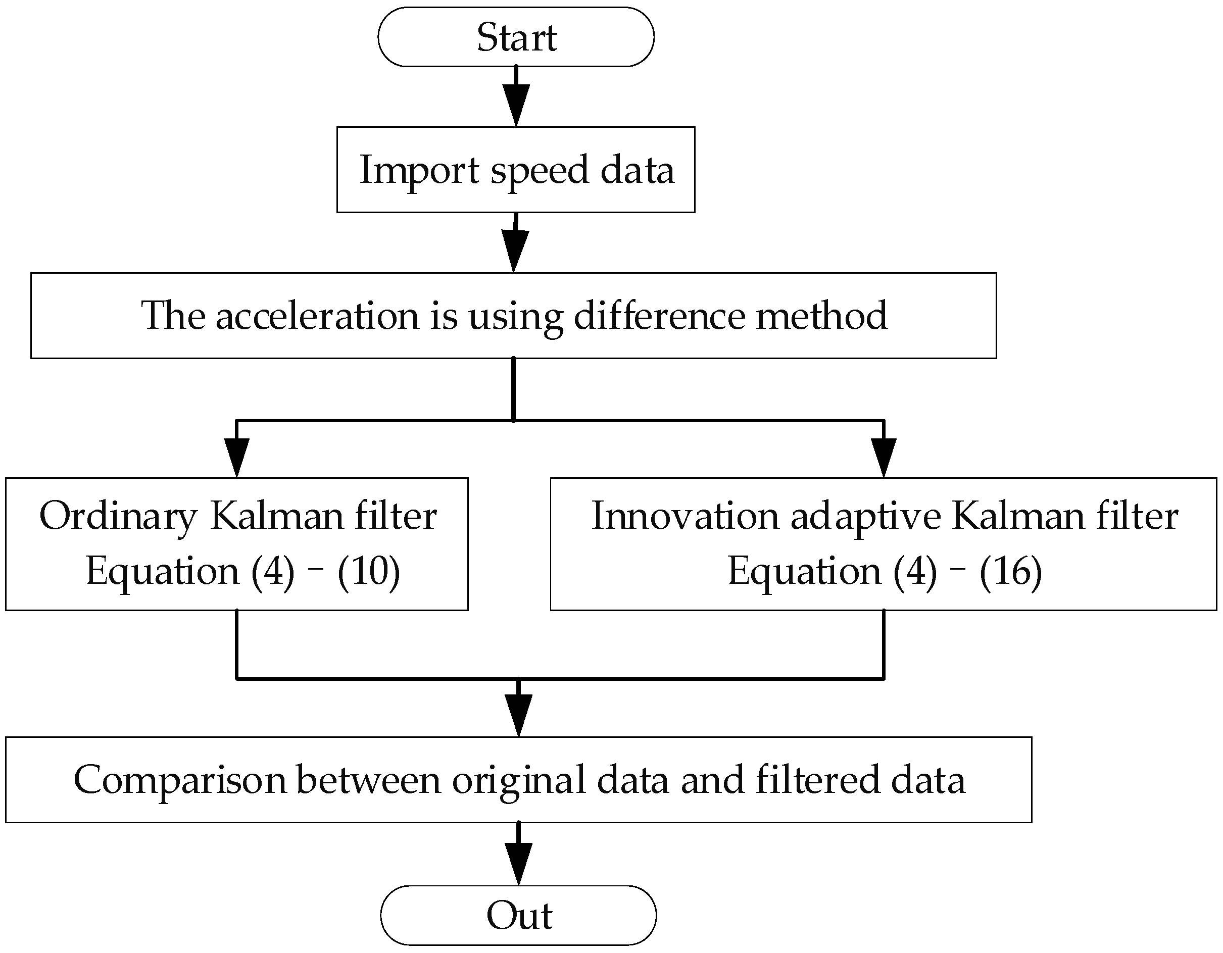
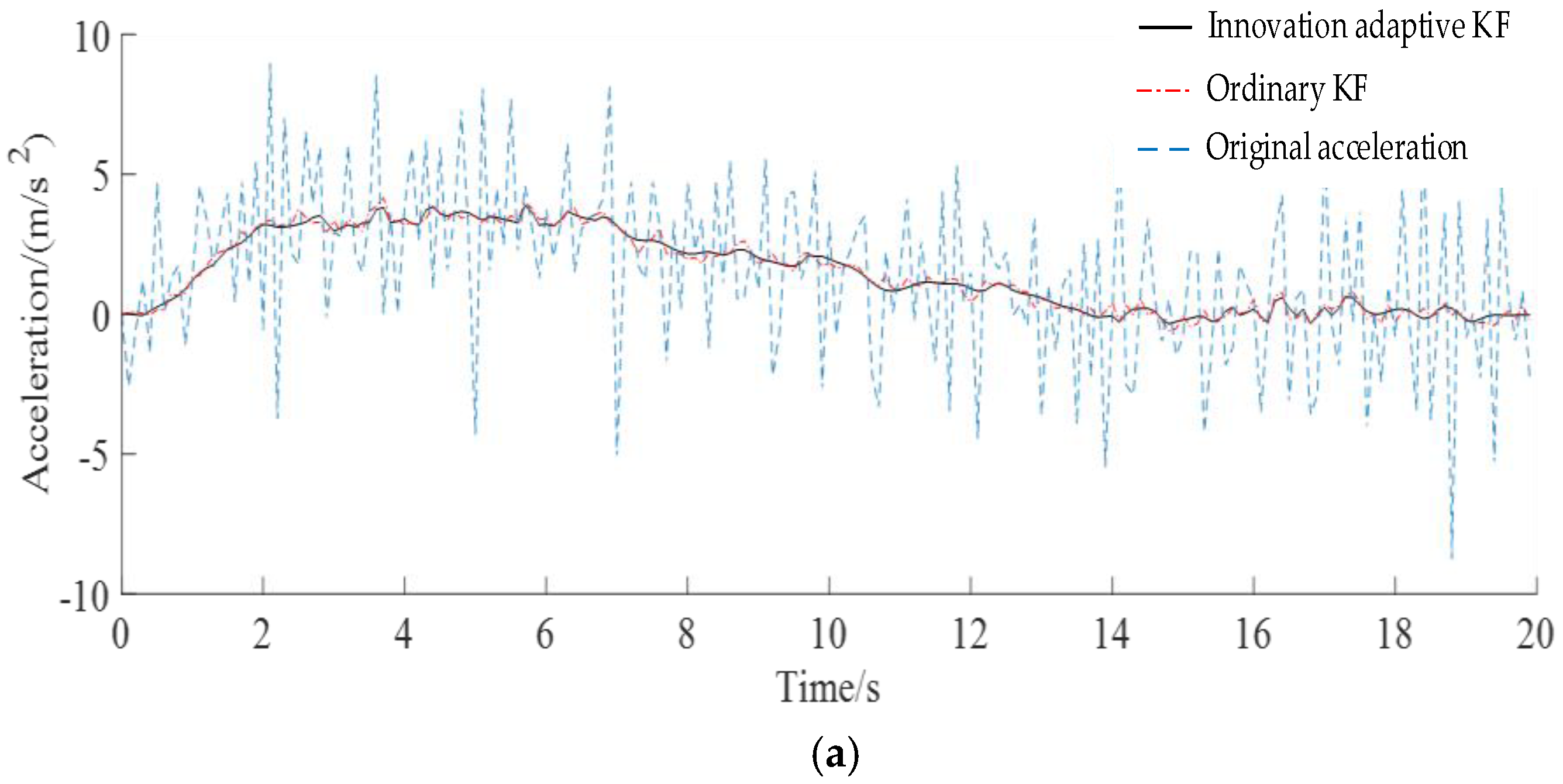
4.1. Simulation Verification

To validate the effectiveness of the adaptive KF algorithm based on innovation covariance, sets of vehicle data are processed using the conventional KF algorithm and the adaptive KF algorithm based on innovation covariance respectively. The resultant velocity and acceleration signals are subsequently compared and analyzed against the original data. The simulation process based on MATLAB R2021a is shown in Figure 2.

Firstly, a set of time-varying speed data is imported into MATLAB R2021a, representing the speed collected by the chassis dynamometer. This dataset consists of 200 speed measurements, reflecting the speed trend throughout 20 s, with a measurement interval of 0.1 s. Since the original dataset is devoid of noise, Gaussian white noise with a mean of 0 and a variance of 0.2 is introduced to simulate the environmental disturbances encountered during the actual operation of the chassis dynamometer. Subsequently, the difference in speed is calculated to derive the acceleration of the vehicle. Blue curves representing the original vehicle speed and acceleration over time are illustrated in Figure 3.

As shown in Figure 3, the acceleration derived from the differential calculation exhibits significant noise. If this acceleration is utilized directly to compute the simulated road resistance, the resistance will fluctuate drastically, preventing the AC motor from responding adequately, which will adversely impact the test results. Therefore, it is essential to apply KF to the initial values in order to reveal the true pattern of change.

The initial acceleration values, as observed, are input into both the standard KF and the adaptive KF based on the innovation, respectively. It is assumed that the error in the vehicle acceleration followed a Gaussian distribution with a mean of 0 and a variance of U. Given that the initial time covariance P(0) has a negligible impact on the filtering effect, the system can rapidly converge as the iterations advance. In setting U = 0.04, the optimal estimate of the acceleration is achieved following the filtering process. The filtered acceleration signal is employed for time integration to derive the new vehicle speed. The resulting curves representing the variations in filtered acceleration and speed over time are depicted in red and black in Figure 3, respectively.

Compared with the original signal, the Gaussian white noise, which is amplified through the differentiation process, is effectively filtered out following ordinary KF. Consequently, the temporal variations in acceleration are discernible, exhibiting a relatively smooth transition that conforms to the acceleration patterns typical of conventional vehicles. However, owing to the inherent limitations of conventional KF in adjusting the noise variance parameters Q and R, there are still certain glitches in the curve. Following the adaptive KF based on innovation covariance, the variance of the innovation is continually assessed, resulting in a more precise noise model. It can be seen that the curve changed smoothly based on the following original signal. Meanwhile, the filtered speed curve exhibits fewer glitches and a smoother profile, thereby confirming the effectiveness of the adaptive KF prediction algorithm based on innovation covariance.

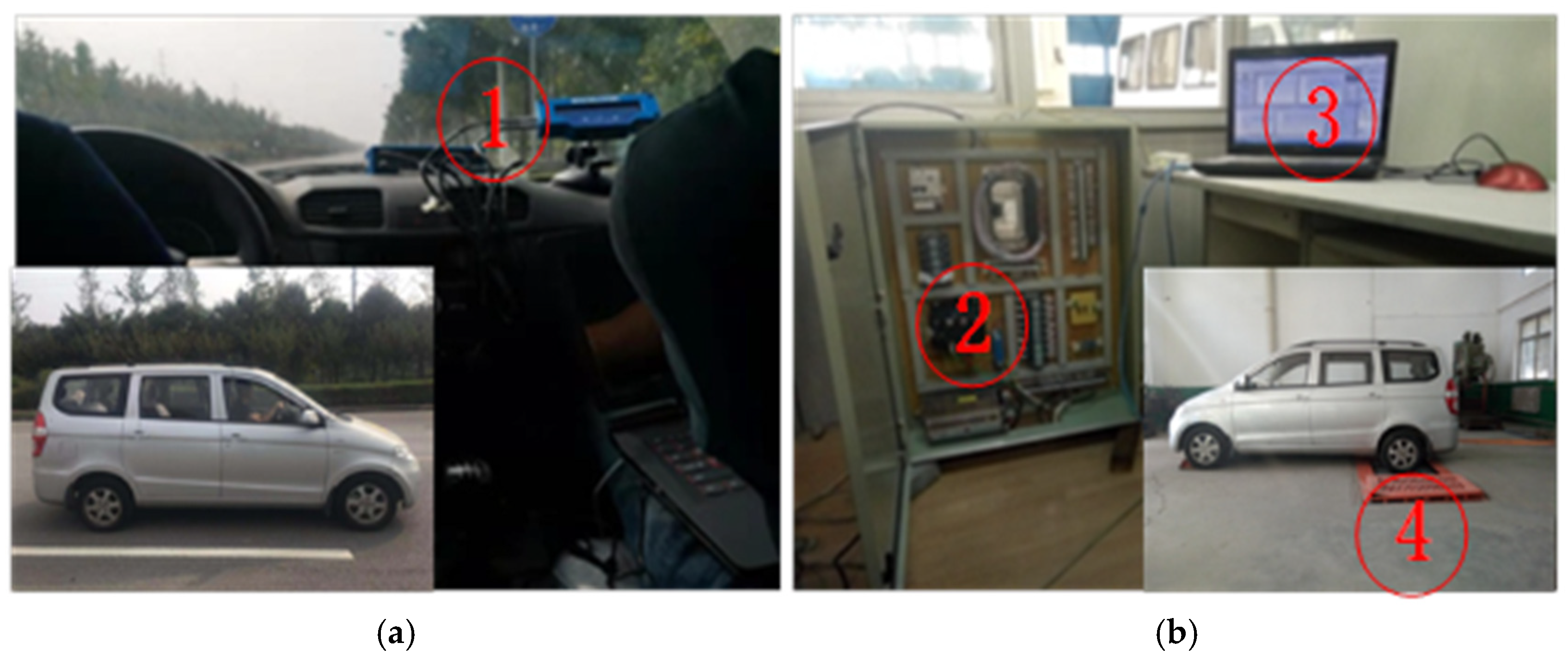
4.2. Test Verification

To further verify the influence of the innovation-based adaptive KF algorithm on the test error, the 2015 SGMW-Wuling Hongguang was used as the test vehicle. Acceleration tests were conducted on both the road and the AC chassis dynamometer, with the testing locations illustrated in Figure 4. Using the road test acceleration time as a reference, the effectiveness of the algorithm was validated by comparing the errors in the acceleration times of the test vehicle before and after the implementation of the KF algorithm with the loading force model.

(a) Road test

The GPS-based VBOX-3i data acquisition system was employed during the road test. In accordance with national standards, the test vehicle was outfitted with the necessary equipment and preheated, subsequently undergoing three round-trip coasting test and acceleration tests. The experimental results are shown in

Table 1. Road coasting test results.

Serial Number	Speed Range (km/h)	65–55		55–45		45–35		35–25		25–15		15–5
		Go	Back	Go	Back	Go	Back	Go	Back	Go	Back	Go	Back
1	Cumulative coasting time (s)	12.7	12.6	28.2	28.7	48.3	49.1	71.0	70.7	97.7	98.1	128.0	128.6
2	Cumulative coasting time (s)	12.9	13.0	29.0	29.2	48.6	48.9	70.8	71.3	98.1	98.2	127.9	129.0
3	Cumulative coasting time (s)	12.5	12.6	28.9	28.6	48.3	48.8	71.3	70.8	97.9	97.6	128.3	128.2
	Average coasting time (s)	12.7		28.75		48.65		71.0		97.9		128.35

and

Table 2. Road acceleration test results.

Serial Number	Speed (km/h)	10		20		30		40		50		60		70
		Go	Back	Go	Back	Go	Back	Go	Back	Go	Back	Go	Back	Go	Back
1	Time (s)	1.1	1.2	2.0	2.1	3.1	3.0	4.9	5.0	6.1	6.0	8.1	8.0	11.0	10.9
2	Time (s)	1.0	1.1	2.1	2.0	3.2	3.0	5.0	4.8	6.3	6.2	8.0	8.1	10.8	11.1
3	Time (s)	0.9	1.1	1.9	2.1	3.0	2.9	5.1	5.0	5.9	6.1	7.9	8.2	10.9	11.1
	Average time (s)	1.1		2.0		3.0		4.9		6.1		8.1		11.0

. The speed of the vehicle and corresponding time are recorded individually, and average values are utilized. The results from the road coasting test are used for curve fitting to obtain coefficients A₁, B₁, and C₁ in Equation (1). The results from the road test serve as a benchmark for comparison.

To ensure the validity of the test results, a repeatability analysis of the data from multiple trials is required. In this study, the 95th percentile distribution method was used for the repeatability assessment. Taking the road acceleration test results as an example, the test was conducted three times. Based on tabulated values, the standard deviation in the acceleration time corresponding to the vehicle speed is 0.063 Q, where Q represents the arithmetic mean of the results from the three repeated tests. The computed standard deviations are 0.0693, 0.126, 0.189, 0.3087, 0.3843, 0.5103, and 0.693, while the corresponding ranges are 0, 0, 0, 0.1, 0.25, 0.15, and 0.15. These ranges are all smaller than the respective standard deviations, indicating good repeatability of the three acceleration test results. Therefore, the vehicle acceleration test data are deemed valid. Likewise, it can be concluded that the coasting test data are also valid.

Based on the road coasting test results, the least squares method was applied in MATLAB R2021a to fit the test data with a polynomial, and the values of A₁, B₁, and C₁ in Equation (1) were obtained as 140.83, −0.40, and 0.06, respectively.

(b) Chassis dynamometer test

Through the use of the chassis dynamometer coasting method and the vehicle coasting without a load and with a secondary load on the chassis dynamometer, the least squares method can be applied to fit the test data to obtain that A₂, B₂, and C₂ in Equation (2) are 530.88, −0.96, and 0.01, respectively. Combined with the relevant parameters of the test vehicle, M is 810 kg, and α, β, and γ are −390.05, 0.56, and 0.05, respectively, and the loading force model of the AC chassis dynamometer is obtained.

The test vehicle was correctly fixed on the AC chassis dynamometer, and its operational condition was adjusted to closely resemble that of the road test. Subsequently, the acceleration performance test was conducted. The loading force model was established in the upper computer of the chassis dynamometer according to Equation (3), and the AC motor was controlled through the inverter to load the drum. Regarding the speed and acceleration motion parameters, both direct loading (the speed and acceleration values directly measured with the sensors) and the innovative adaptive KF prediction algorithm were employed to determine the optimized values of the loading force model. This test was conducted three times. The speed and time were recorded individually, and their average values were computed. The experimental results are shown in

Table 3. Direct load acceleration test results of chassis dynamometer.

Serial Number	Speed (km/h)	10	20	30	40	50	60	70
1	Time (s)	0.9	1.5	2.4	4.5	5.4	7.8	10.3
2	Time (s)	1.1	1.6	2.7	4.7	5.8	7.4	10.4
3	Time (s)	0.7	2.0	2.7	4.3	5.9	7.6	10.2
	Average Time (s)	0.9	1.7	2.6	4.5	5.7	7.6	10.3

and

Table 4. Innovative adaptive KF algorithm acceleration test results of chassis dynamometer.

Serial Number	Speed (km/h)	10	20	30	40	50	60	70
1	Time (s)	1.1	1.8	2.8	4.9	6.3	7.9	11.4
2	Time (s)	1.2	1.9	3.3	5.3	6.3	8.4	11.0
3	Time (s)	1.3	2.3	3.2	5.1	6.3	8.3	11.2
	Average Time (s)	1.2	2.0	3.1	5.1	6.3	8.2	11.2

. The three sets of test data were then plotted to create a time–speed curve, as depicted in Figure 5.

The deviation relative to the road test acceleration time served as the evaluation index, and the test error was defined as

$$\sigma ={\displaystyle \frac{\left|t-t_0\right|}{t_0}}$$

(22)

where σ is the test error, t is the acceleration time of the chassis dynamometer, s; and t₀ is the road test acceleration time, s.

It can be intuitively seen from Figure 5 that, when using the actual road test acceleration time as a reference, the acceleration time of the direct loading scheme exhibits significant discrepancies. In contrast, the optimized acceleration time derived from the loading force model closely approximated that of the road test. As the velocity reached 70 km/h, the error of the optimized loading force model diminished from 6.4% to 1.8%. This demonstrates that the adaptive KF prediction algorithm based on innovation covariance could effectively optimize the loading force model of the chassis dynamometer, thereby enhancing its accuracy.

5. Conclusions

The adaptive KF algorithm, based on innovation covariance, was employed in vehicle chassis dynamometer testing to estimate the motion parameters of the test vehicle. Following simulation and experimental validation, the following conclusions were reached:

(1) The loading force model of the chassis dynamometer was established through an analysis of the principles of the chassis dynamometer and subsequently optimized using the adaptive KF algorithm based on innovation covariance.

(2) The innovation-based adaptive KF algorithm effectively mitigates the Gaussian white noise amplified by the velocity differential operation, allowing for a more precise estimation of the motion parameters of the vehicle. Additionally, it optimizes the loading force model within the measurement and control system of the chassis dynamometer.

(3) The test error of the chassis dynamometer can be reduced from 6.4% to 1.8% by employing the adaptive KF algorithm based on innovation covariance. This improvement significantly enhances the testing accuracy of the chassis dynamometer, demonstrating the effectiveness of the algorithm in refining measurement precision.

References

1. Li, B. Research on Objective Test and Evaluation Method of Vehicle Drivability Based on Chassis Dynamometer. Master’s Thesis, Hefei University of Technology, Hefei, China, 2022. [Google Scholar]
2. Zhou, L.; Guo, H.; Zhao, H.; Ma, M. A Review of Research on Dynamometer System. Electr. Mach. Control. Appl. 2020, 47, 1–9. [Google Scholar]
3. Zhang, S.; Zhang, X.; Xu, L.; Yan, X. Research on AC chassis dynamometer system based on virtual prototype. Mod. Manuf. Eng. 2022, 9, 123–131. [Google Scholar]
4. Lourenço, M.A.d.M.; Eckert, J.J.; Silva, F.L.; Santiciolli, F.M.; Silva, L.C.A. Vehicle and twin-roller chassis dynamometer model considering slip tire interactions. Mech. Based Des. Struct. Mach. 2022, 51, 6166–6183. [Google Scholar] [CrossRef]
5. Huang, W.; Liu, D.; Chu, R.; Qiu, F.; Li, Z.; Jin, X.; Zhang, H.; Wang, Y.; Ji, S. Analysis of Resistance Influencing Factors of a Bench System Based on a Self-Developed Four-Wheel Drive Motor Vehicle Chassis Dynamometer. Machines 2024, 12, 580. [Google Scholar] [CrossRef]
6. Casadei, S.; Maggioni, A. Performance Testing of a Locomotive Engine Aftertreatment Pre-prototype in a Passenger Cars Chassis Dynamometer Laboratory. Transp. Res. Procedia 2016, 14, 605–614. [Google Scholar] [CrossRef]
7. Akpolat, Z.H.; Asher, G.; Clare, J. Dynamic emulation of mechanical loads using a vector-controlled induction motor-generator set. IEEE Trans. Ind. Electron. 1999, 46, 370–379. [Google Scholar] [CrossRef]
8. Hewson, C.; Wheeler, P.; Asher, G.; Sumner, M. Dynamic mechanical load emulation test facility to evaluate the performance of AC inverters. Power Eng. 2000, 14, 21–28. [Google Scholar] [CrossRef]
9. Zhang, L.; Li, L.; Zhang, T. The application of human-like intelligent control in motorcycle chassis dynamometer. Autom. Instrum. 2006, 128, 65–71. [Google Scholar]
10. Zheng, Z.W. Research on Application of Fuzzy Control Theory in Automobile Chassis Dynamometer System. Master’s Thesis, South China University of Technology, Guangzhou, China, 2010. [Google Scholar]
11. Li, L. DTC Control System of Energy-Feeding AC Chassis Dynamometer. Master’s Thesis, Chongqing University, Chongqing, China, 2010. [Google Scholar]
12. Li, Z.; Geng, Y.; Shi, W. Design of a prototype measurement and control platform for rapid control of automobile chassis dynamometer. Mech. Des. Manuf. Eng. 2018, 4, 162–164. [Google Scholar] [CrossRef]
13. Huang, P.; Ding, W.; Wang, X.; Teng, X. Review of interferometric synthetic aperture sonar interferometric phase filtering methods. Adv. Mech. Eng. 2023, 15. [Google Scholar] [CrossRef]
14. Kumar, M.; Mishra, S.K. A Comprehensive Review on Nature Inspired Neural Network based Adaptive Filter for Eliminating Noise in Medical Images. Curr. Med. Imaging Former. Curr. Med. Imaging Rev. 2020, 16, 278–287. [Google Scholar] [CrossRef]
15. Zhao, J.; Lei, Y.; Li, Z. Survey on Application of Kalman Filter in Equipment Fault Prediction. Ordnance Ind. Autom. 2024, 43, 16–20. [Google Scholar]
16. Zhang, H.; Zhang, H. Research and Application of Differential Tracker. Control. Instrum. Chem. Ind. 2013, 40, 474–477. [Google Scholar]
17. He, Y.; Han, J. Experimental Study of Angular Acceleration Estimation based on Kalman Filter and Newton Predictor. Chin. J. Mech. Eng. 2006, 42, 226–232. [Google Scholar] [CrossRef]
18. Zhang, X.; Zhou, Z. Speed control strategy for tractor assisted driving based on chassis dynamometer test. Int. J. Agric. Biol. Eng. 2021, 14, 169–175. [Google Scholar] [CrossRef]
19. Zheng, X.X. Research on Test Technology of Chassis Dynamometer Based on Dynamic Loading of Rolling Resistance and Prediction of Motion Parameters. Master’s Thesis, Zhejiang University, Hangzhou, China, 2018. [Google Scholar]
20. Bisht, S.S.; Singh, M.P. An adaptive unscented Kalman filter for tracking sudden stiffness changes. Mech. Syst. Signal Process. 2014, 49, 181–195. [Google Scholar] [CrossRef]
21. Wang, X.D. Simulating the Road Resistance of Commercial Vehicles with the Dynamometer and Studying the Load Force. Master’s Thesis, Changan university, Xi’an, China, 2010. [Google Scholar]
22. Archibald, R.; Bao, F.; Tu, X. A direct filter method for parameter estimation. J. Comput. Phys. 2019, 398, 108871. [Google Scholar] [CrossRef]
23. Euler-Rolle, N.; Mayr, C.H.; Škrjanc, I.; Jakubek, S.; Karer, G. Automated vehicle driveaway with a manual dry clutch on chassis dynamometers: Efficient identification and decoupling control. ISA Trans. 2020, 98, 237–250. [Google Scholar] [CrossRef]
24. Hernandez-Barragan, J.; Rios, J.D.; Alanis, A.Y.; Lopez-Franco, C.; Gomez-Avila, J.; Arana-Daniel, N. Adaptive Single Neuron Anti-Windup PID Controller Based on the Extended Kalman Filter Algorithm. Electronics 2020, 9, 636. [Google Scholar] [CrossRef]
25. Xiao, X.; Sun, Z.; Shen, W. A Kalman filter algorithm for identifying track irregularities of railway bridges using vehicle dynamic responses. Mech. Syst. Signal Process. 2020, 138, 106582. [Google Scholar] [CrossRef]
26. Cao, Q.; Zhou, Z.; Zhang, M.; Xi, Z.; Xi, J. Estimation method and verification of slip ratio of tractor driving wheel. J. Agric. Eng. 2015, 31, 35–41. [Google Scholar]
Figure 1. Schematic of AC chassis dynamometer.
Wevj 16 00239 g001
Figure 2. Simulation flow chart.
Wevj 16 00239 g002
Figure 3. Simulation results before and after filtering algorithm: (a) Vehicle acceleration. (b) Vehicle speed.
Wevj 16 00239 g003aWevj 16 00239 g003b
Figure 4. Test Site: ① VBOX-3i; ② data acquisition controller; ③ upper computer; ④ chassis dynamometer bench. (a) Road test. (b) Chassis dynamometer test.
Wevj 16 00239 g004
Figure 5. Comparison of test data.
Wevj 16 00239 g005