Abstract
By applying the wavelet tool, this study examines the effect of foreign direct investment (FDI) on pollution in China, for the period 1982 to 2016. Carbon dioxide and sulfur dioxide emissions are used as pollution variables. The results reveal that FDI positively affected pollution at high frequency (short term) during the 1980s and after 2000, and at low frequency (long term) but not at medium frequency (medium term) for the entire time period. It demonstrates that FDI increases pollution both in the short and long term, but not in the medium term. It indicates that FDI has created pollution havens in China. For robustness analysis, spectral causality test was applied. The results of this causality test indicate that FDI causes CO2 emissions both in the short-run and long-run. This suggests that in China FDI predicts CO2 emissions. Thus, stringent environmental rules are required to restrict the inflows of foreign dirty industries in China.
1. Introduction
For sustainable economic development, improvement in environmental quality is indispensable. There are different factors which affect environmental quality, such as economic growth, industrial production, energy consumption, financial development, etc. Besides national economic activities, international economic activities also affect the environment. So, there is a need to examine interrelations between transboundary economic activities such as capital flows, trade, finance, transport, etc. and domestic environment. Foreign direct investment (FDI) is also an international activity which is indispensable for economic growth, however, it also affects the environment of the host country. FDI inflows increase domestic production, which increases the burning of fossil fuels in domestic industries. It increases the pollution levels, which deteriorates the environmental quality.
There are basically two competing theories regarding the impact of FDI on environmental quality in host country i.e., the pollution haven hypothesis and the pollution halo hypothesis [1,2]. Pollution haven hypothesis stipulates that FDI aggravates pollution in developing countries because these countries attract foreign investment by lowering their environmental standards. Empirically, many studies have supported the pollution haven hypothesis (see e.g., [3,4,5,6,7,8,9,10,11,12]). In turn, some studies have criticized the pollution haven hypothesis and have not supported this hypothesis [13,14]. According to the pollution halo hypothesis, FDI transfers high technology and diffuses best management practices in the host countries, which create pollution halos to reduce pollution by exerting positive externalities. Many empirical studies have also supported the pollution halo hypothesis [7,15,16].
FDI affects environmental quality through different channels i.e., scale effect, composition effect and technique effect [17]. According to scale effect, FDI increases pollution by simply scaling-up the economy, ceteris paribus [15]. The composition (structural) effect stipulates that FDI can increase or decrease pollution by changing the pattern of economic activity [18]. For instance, if foreign firms use labor-intensive (capital-intensive) production methods, then pollution will decrease (increase). The technique effect postulates that foreign firms may bring more environmentally friendly techniques, which will also have spillover for local firms [19]. It will improve the environment by reducing emission as resources will be efficiently utilized, and thereby less pollution will be emitted. FDI also affects pollution through another channel, which is called income effect. According to this effect when income increases due to FDI, people demand more stringent regulations and high environmental standards, which reduces pollution. Thus, the effect of FDI on pollution is complex and depends upon which effect dominates the other effects. If the technology effect dominates then FDI will decrease pollution. However, if scale effect dominates then pollution will increase with FDI.
This theoretical trade-off has stimulated researchers to empirically investigate the effect of FDI on the environment in the host country. Some studies have shown that FDI inflows increase pollution [9,16,20,21], while others have shown that FDI inflows reduce pollution [22,23,24]. Thus, like theoretical literature, empirical literature has also provided mixed results about the impact of FDI on environment in the host country. Empirical findings in China have also shown mixed results. Some studies have shown that FDI has turned China into a pollution haven as it has deteriorated the environment by contributing to pollution, while other studies have supported the pollution halo hypothesis and have shown that FDI has improved the environment by decreasing pollution through transfer of technology. Section 3 provides the literature review for China in detail.
Although some studies have been conducted to examine the effect of FDI on the environment in China, more empirical analysis is required for several reasons. Firstly, empirical literature has provided contradictory results for the effect of FDI on the environment in China. Thus, there is a need to re-examine the association between FDI and the environment. Secondly, almost all studies in China have used panel data, but examining the FDI–environment link using time series data for China will provide useful policy implications. The advantage of time series analysis is that it is useful for explanative analysis, that is, it helps to study cross-correlation and relationship between two time-series and their dependence on each other. Furthermore, time series analysis helps to understand the past and to predict the future. Thirdly, previous studies in China have used traditional analysis techniques such as regression analysis using OLS, panel fixed effect, random effect, Generalized Method of Moments (GMM), etc. This study is the first study which will use the wavelet coherence technique to examine the FDI-environment linkages. The wavelet coherence approach helps to identify the lead-lag relationship between the variables over time and across frequencies. The latter aspect highlights the dependence dynamics of variables from a short, medium and long run perspective, and thus assists in formulating the policies accordingly. Fourthly, previous studies have used annual data for the analysis, while the present will use quarterly frequencies for empirical analysis. The study will help China to formulate its future pollution abatement policy.
2. FDI and Pollution in China
Since its reforms for opening up its economy in 1978, the level of FDI has increased in China for last three decades. FDI, which was just $0.43 billion in 1982 increased to $11 billion in 1992. FDI decreased in the late 1990s, due to the Asian financial crisis, but started increasing again in the 2000s and has maintained a steady upward trend since then. FDI increased from $53 billion in 2002 to $291 billion in 2013, which is the highest of all time, for FDI inflows in China. In 2017, $144 billion entered into China in terms of FDI inflows, which has made it the world’s second largest recipient of FDI after the USA [25].
Thus, FDI has become an important component of the Chinese economy over the past three decades [11]. It has provided the financial resources for economic growth. It has stimulated technological innovations, created employment opportunities, improved the skills of laborers, promoted trade especially exports, upgraded management skills both in public and private institutions, and helped to eradicate poverty levels in the country. Figure 1 depicts the pattern of both GDP growth and FDI inflows (% of GDP). It is evident from the figure that when FDI increases, income growth also increases, especially, after 1990 when FDI surged. Both FDI and economic growth followed the same pattern i.e., when FDI increases economic growth also increases and vice versa. FDI inflows have not only increased the overall economic growth of the country but have also increased the per capita income of the country. Figure 2 depicts the trend of both per capita income and FDI. It is clear from the figure that both FDI and per capita income follow the same pattern i.e., when FDI increases, then per capita income also increases. Per capita income, which was $203 in 1982, it increased to $1148 in 2002 and further increased to $8123 in 2016. This pattern continued until 2014, after which FDI started declining, due to the global decline in FDI inflows.
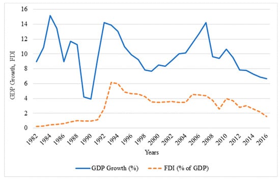
Figure 1.
GDP Growth (%) and foreign direct investment (FDI) (% of GDP).
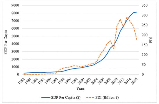
Figure 2.
GDP Per Capita ($) and FDI (Billions $).
FDI also has some problems and impediments in China. Some important issues are regional imbalance, imbalance in sectoral distribution, abuse of transfer pricing, and implications for competition in the domestic market. This high inflow of FDI is also accompanied by environmental deterioration [6]. Most of the foreign investment is invested in pollution emitting industries, which has deteriorated the environment [26,27]. China has become the largest carbon emission country in the world in 2017, sharing 30% of world carbon emissions. Carbon emissions have increased from approximately 2,442,431 (kt) in 1990 to 10,745,401 (kt) in 2016. In per capita terms, carbon emission has increased from 2.15 metric tons in 1990 to 8.09 metric tons in 2016. Figure 3 explains the pattern of carbon emissions in China, which clearly indicates that both CO2 (kt) and CO2 per capita (metric tons) have increased over time, in the wake of FDI inflows in the country. After joining World Trade Organization (WTO) in 2001, Chinese exports have increased globally, which has also increased carbon emissions.
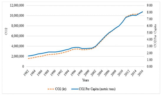
Figure 3.
CO2 (kt) and CO2 Per Capita (metric tons).
Air pollution in China is also worst in the world and has become a threat to public health. In China, PM2.5 concentration is 5 times higher than world health organization (WHO) standards, which is 10 micrograms per cubic meters. In 2015, 1.6 million deaths occurred in China due to air pollution. In 2016, out of 338, only 84 cities maintained air quality standards. Air pollution is worst in the northern industrial provinces of the country. Figure 4 explains the pattern of SO2 emissions in China. SO2 rapidly increased in the country between 1995 and 2006, a period during which FDI inflows also surged in the country. After 2006, SO2 started declining mainly due to the adoption of flue-gas desulfurization technology by power plants. Further, China is shifting from coal, which is the major source of air pollution, to other energy sources such as hydro, wind, solar, nuclear, etc. Figure 5 explains that, like SO2, total greenhouse gas (GHG) emissions (kt of CO2 equivalent) have also increased in China with the inflow of FDI. Total GHG has increased by 5 times in 2016 compared to its level in the early 1980s. GHG increased at a faster rate after 2001 when China joined the WTO. All it indicates, it that FDI has vandalized the environment in China.
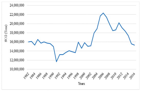
Figure 4.
Sulfur Dioxide (SO2) Emissions (tons).
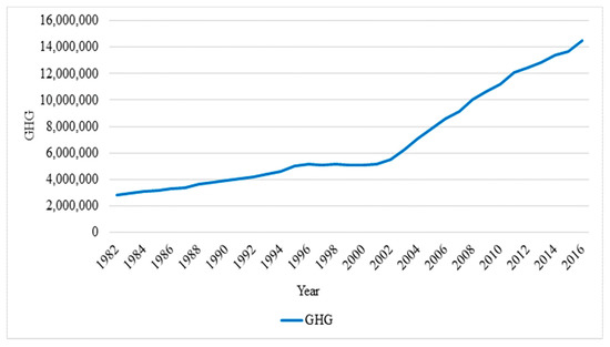
Figure 5.
GHG Emissions.
Environmental damage has become a serious issue in China. China had previously shown efforts to curb pollution, but in the early 2010s, China started taking serious steps to reduce pollution. To deal with the pollution issue, the Chinese government has introduced several measures. One important step is the introduction of the electric vehicle in the country. Since 2015, China has become the global leader in sales of electric vehicles. China is also cutting excess industrial capacity, which will help to clean the environment by reducing coal consumptions. The Chinese government has also taken steps to reduce pollution in its 13th five-year plan, which was announced in November 2016. In this plan, special emphasis was given to reduce air pollution by reducing PM2.5 in the 10 worst affected cities of China by 18 percent and by reducing coal production by 140 million tons by 2020. To alleviate air pollution China has also closed 40 percent of its industrial units which were contributing to pollution. Furthermore, the Chinese government will spend $367 billion on renewable power projects which will also help to decrease dependence on coal consumption for power generation, to less than 40 percent by 2040, compared to the current 70 percent (Data is taken from https://chinapower.csis.org/air-quality/). Previously, in 2015, an Environmental Protection Law was also introduced to curb pollution. Although the government has taken many steps to curb pollution, still more needs to be done in this regard.
3. Literature Review
Empirically, many studies have examined the effect of FDI on environmental pollution. Some of them have supported the Pollution Haven Hypothesis (see e.g., [3,4,5,6,7,8,9,12,16,20,28,29,30,31,32,33,34,35,36,37,38]). Other studies have supported the Pollution Halo Hypothesis and suggest that FDI is accompanied by green technologies which improves environmental conditions [22,23,24,33,39,40,41,42]. According to Hoffmann et al. [43] the impact of foreign investment on pollution is contingent upon the level of development, as the pollution haven hypothesis holds only for less developed countries, not developed countries. According to Kim and Adilov [44] both the pollution haven and the pollution halo hypotheses may hold together in developing countries.
Empirical literature is also available for China. Table 1 provides a summary of the literature review for China (See Sung et al. [45] for a recent literature review for other countries). It is evident from this table that different studies have provided contradictory results. Recently, Liu et al. [46] have also shown that FDI has different effects on distinct pollutant variables, as FDI has decreased dust pollution and waste soot, while it has increased waste water and air pollution. Similarly, Yang and Wang [47] have found that FDI has increased air pollution and has decreased solid waste. Zhang and Zhou [24] documents that FDI has decreased pollution in China. Recently, Zheng and Sheng [48] have shown that FDI has increased China’s pollution after market-oriented reforms. But this effect has gradually decreased over time.

Table 1.
Literature Review.
Wang and Chen [11] reveal that investments from Organization for Economic Co-operation and Development (OECD) countries have increased pollution, but FDI from Hong Kong, Macau, and Taiwan (HMT) has not affected the environment. The study suggests that institutional development reduces the detrimental impacts of FDI on environment. In contrast, Huang et al. [49] have shown that FDI from HMT decreases pollution while FDI from other origins has no measurable impacts on the environment. Dean et al. [50] indicate that FDI from HMT increases pollution as FDI from these countries is attracted to areas with lax environment rules, while FDI from OECD countries decreases pollution. Lan et al. [6] show that the effect of FDI on pollution in China depends upon the level of human capital. FDI improves (deteriorates) environment in provinces which have high (low) level of human capital.
In brief, the empirical literature is inconclusive about the impact of FDI on pollution in China. This inconclusive evidence is due to differences in research objectives, estimation techniques, pollutant variables, time period, data types (panel vs. times series), heterogeneity in panels, number of provinces/cities considered, sectors covered, control variables taken, etc. Thus, there is a need to further probe the linkages between FDI and pollution in China, as China is the world’s largest recipient of FDI and pollution emitting county. In this paper, our main concern is about the estimation technique, as previous studies have used traditional econometric techniques to check FDI-pollution linkages. The present study will apply a more sophisticated technique called wavelet coherence to gauge the association between these two variables.
4. Methodology
4.1. Continuous Wavelet Transformation
We probe the dynamic interaction between FDI and pollution using time–frequency analysis, namely the wavelet approach. This time–frequency approach helps to examine the dynamic links between variables over time and across different frequencies [59].
For a time series the continuous wavelet transformation (CWT) for wavelet is expressed as:
indicates the time domain of the wavelet while indicates the frequency domain of the wavelet. In this way, wavelet transformation gives us information simultaneously about time and frequency. An important concept in the wavelet domain is the wavelet power spectrum (WPS) which is defined as follows:
WPS measures the contribution at each time and scale to time series’ variance.
4.2. Wavelet Coherence and Phase Difference
The wavelet coherence (WTC) is denoted by and is defined as
with . The phase difference is defined as
Here , hence it is called phase difference. Where and are calculated as and , respectively. This relation holds when is converted into an angle in the interval . and represent the real and imaginary part of a complex number, respectively. Two time series move together when the phase difference is zero, at a specified frequency. The series are in phase and leads when , and leads for , respectively. In contrast, the series are in anti-phase, when the phase difference is or . Therefore, leads for , and leads when , respectively.
4.3. Wavelet Cohesion and Wavelet-Based Causality
The causality measure is based on the CWT correlation measure of Rua [60]. The wavelet correlation measure of Rua [60] is provided as:
lies between −1 and 1 i.e., . This correlation measures indicates co-movements both at frequency and over time. The Granger causality measure of Olayeni [61] in CWT framework is an extension of the wavelet-based correlation measure of Rua [60]. The CWT–Granger causality measure is expressed as:
where denotes an indicator function, which is defined as follows:
As can be seen, the main difference between the wavelet correlation and the CWT–Granger causality measure is the inclusion of the causal information through the indicator function .
5. Empirical Results
5.1. Data and Preliminary Statistics
We use two measurements of FDI i.e., the amount of FDI and FDI (% of GDP) to comprehensively capture its effect on pollution. The amount of FDI is extensively used to measure the size of foreign financial inflows in the recipient country [62]. Following Cole et al. [63], we also take FDI (% of GDP) to see the relative importance of foreign capital inflows in the recipient country’s economic activity. Since carbon emission is an important source of global pollution, we use CO2 emission to measure pollution. Two measures of CO2 emission are used i.e., CO2 emissions (kt) and per capita CO2 emissions (metric tons). These indicators are widely used in the environmental literature. Further, we have also considered SO2 emission to measure air pollution. Data for FDI and CO2 variables is taken from the World Bank and the data for SO2 is taken from China Environmental Statistics Yearbooks. Initially, annual times series data is collected for the period 1982 to 2016, which is then converted into quarterly frequencies. It gives us 140 observations.
Table 2 provides the descriptive statistics of the variables. The mean value of FDI is $20.80 billion, which ranges between 0.09 and 75.06 billion dollars. Similarly, the mean value of FDI to GDP ratio is 2.87%, which ranges from 0.20% to 7.13%. The mean value of per capita CO2 emission is 3.89, which ranges between 1.55 and 8.23 metric tons per capita. FDI to GDP ratio is the only variable which is normal and all other variables are not normal, as the Jarque–Bera (JB) rejects the null hypothesis of normality for all variables except FDI to GDP ratio. Table 3 provides the correlation matrix of the variables. FDI has a high correlation with all polluting variables and this correlation is highly statistically significant. The FDI to GDP ratio also has statistically significant correlation with all polluting variables, however, the magnitude of this correlation is low compared to the correlation of FDI with pollution variables. Further, the correlation of FDI and FDI to GDP ratio is more with CO2 variables as compared to SO2.
Table 2.
Descriptive Statistics of the Variables.
Table 3.
Correlation Matrix.
5.2. Continuous Wavelet Transformation (CWT) Power Spectrum
The wavelet technique measures association between two non-stationary series, therefore testing the stationarity of the variables is not necessary in a frequency–domain approach [59,64,65,66]. As evident from the previous section, all series have an increasing trend, therefore, for wavelet analysis all series are detrended by taking their log first difference. To examine the power/variance of the variables, the continuous wavelet transformation (CWT) power spectral is plotted. Figure 6 provides the CWT power spectra1 of the FDI and pollution variables. The power spectral of FDI shows that FDI has high and significant variations between 1989 and 1996 at 14–20 quarters of scale (medium frequency or medium term), and 2008–2013 at 0–14 quarters of scale (high frequency or short term to medium frequency). These frequency bands are conventional. The first 4 quarters show high frequency, 4–8 quarters show medium and more than 8 quarters show low frequency bands. Thus, FDI is found to be highly volatile in two periods, but at different frequency levels. During the first period, FDI inflows surged in China and the second period is the period after the recent financial crisis of 2007/08. More or less a similar pattern is found when FDI is taken as share of GDP. Both carbon emission variables have strong and significant power in the short run at 1–6 quarters of scale mainly between 1992–2012. Further, volatility is also high mainly in the long-run (from 32 scale onwards). Volatility for SO2 is high for the period 1987 to 2002 for 1 to 14 quarters (high to medium frequency).
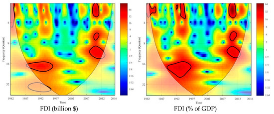
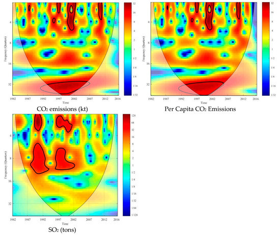
Figure 6.
Continuous Wavelet Transformation (CWT) Power Spectrum of Time Series. Note: The 5% significance level (against the red noise) is depicted by thick black contour. The cone of influence (COI) is shown as a lighted shadow, the area where the edge effects might distort the picture. The color bar shown on the right side of each figure indicates the color code for power that ranges from low power (in blue) to high power (in red). The study time period is on X-axis whereas the Y-axis indicates the frequency (in quarters).
5.3. Wavelet Coherency (WTC)
Figure 7 provides the WTC plots. Panel A provides WTC plots of FDI with pollution variables while panel B provides the WTC plots of FDI (% of GDP) with pollution variables. For WTC of FDI with carbon emission (kt), co-movements have been registered at frequency range of 1–3 quarters during 1984–1986, 1994–1995 and 2010–2011, and at medium frequency (medium term) 8–16 quarters during 2006–2016. The variables have cyclical effects, the arrows being oriented to right and up, FDI causes CO2 emission positively. It shows that FDI increases carbon emissions. The same results hold when per capita carbon emission is used. The results are very interesting for the case of SO2. Co-movements are found for medium frequencies from 1982 to 1997 for 16 to 22 quarters, and for frequencies 1–30 for 2007 to 2016. The arrows being oriented to right and up, FDI causes SO2 positively. It shows that FDI increases SO2 emissions. It re-enforces the hypothesis that FDI leads to pollution in China. The same results are found in Panel B when we use FDI (% of GDP).
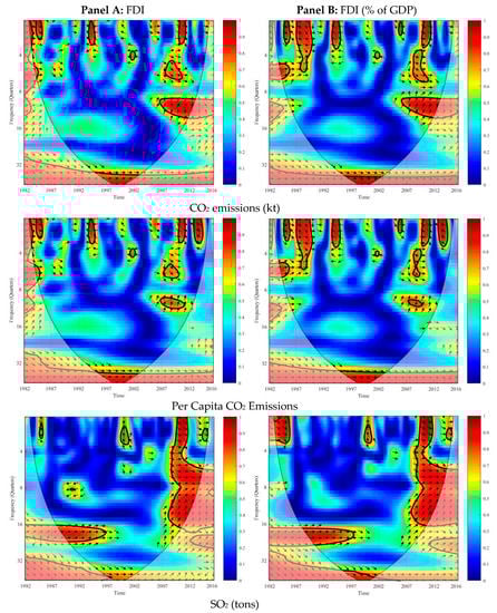
Figure 7.
Wavelet Coherency (WTC) between FDI and Pollution Variables. Note: The 5% significance level is depicted by thick black contour which is estimated through Monte Carlo simulations following phase randomized surrogate series. The phase differences between the two series are shown through arrows. The variables are in phase (out-of-phase) when the arrows are pointed to the right (left). In phase (out-of-phase) implies a positive (negative) relationship. The FDI (CO2 emissions) leads when the arrows point towards the right and up (right and down). The CO2 emissions (FDI) lead when the arrows are pointing towards left and up (left and down). For other details please refer to notes of previous figures.
5.4. Wavelet Causality and Correlations
Figure 8 provides causality results of the wavelet transformation. Panel A presents the causal effects from FDI to pollution variables. The color code shows the strength of causal effects which runs from 0 to 1. For CO2 emission (kt) causal effect is observed between 1982 and 1990 on 26~36 quarters and between 1983 and 2016 on 0~8 quarter frequency and this is a somewhat stronger causal effect. More or less a similar causal pattern holds with per capita CO2 emissions. However, for SO2 a strong causal effect is found between 2007 to 2016 on 0~8 quarter frequency. Panel B reports the causal flow from FDI (% of GDP) to pollution variables. The causal effect of FDI (% of GDP) on pollution variables is strong compared to the effect of FDI.
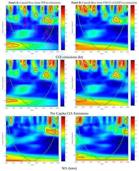
Figure 8.
Wavelet based Causality from FDI to Emissions. Note: The statistical significance at 5% and 10% level (computed based on 1000 Markov bootstrapped series) are indicated through white and red contours, respectively. For other details please refer to the notes of previous figures.
Figure 9 reports the Rua [60] measure of CWT correlation. Panel A provides the correlation of FDI with pollution variables while Panel B provides the correlation of FDI (% of GDP) with pollution variables. It is obvious from these plots that the period of high positive correlation between variables is the same as the periods of causal relations depicted in Figure 8. The plots generally confirm the outcomes in WTC. The first plot in Panel A shows the correlation between FDI and CO2 emission (kt). It is evident that both variables have high positive co-movements during 1982–1992, and 2005–2016 at 1–14 quarters band of scale (high and medium frequency). However, this positive co-movement is persistent for the entire time period at low frequency. No co-movement between FDI and CO2 emission is observed for the remaining sub-periods, which confirms the neutrality hypothesis during these periods. A similar interpretation holds for all variables. However, it is observed that the correlation between FDI variables and SO2 is high compared to the correlation between FDI variables and CO2 variables. It indicates that FDI has vandalized air quality more by emitting sulfur dioxide. These correlation results are somewhat in contrast with the simple correlation results given in Table 3, wherein FDI variables are highly correlated with CO2 variables, as compared to SO2 variables. However, these results are in line with the results of simple correlations that FDI variables are positively correlated with pollution variables.
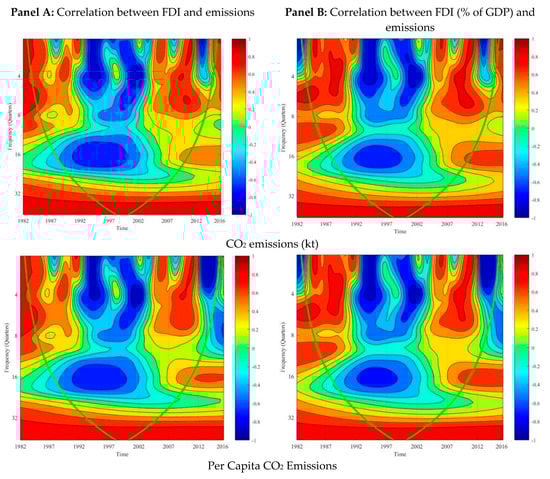
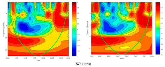
Figure 9.
Wavelet-Based Correlations [60]. Note: The figure shows the wavelet-based correlations [60]. The color code shows the degree of correlations, which goes from blue (negative correlation) to red color (positive correlation).
5.5. Robustness Checks
For robustness analysis, we have applied the Breitung and Candelon [67] spectral causality test. This test decomposes the causality test statistics into different frequencies. Breitung and Candelon [67] have suggested the estimation of the frequency domain causality by imposing linear restrictions on the autoregressive parameters in a Vector Autoregression (VAR) model, allowing for causality testing at different frequency bands that differ between short-, medium- and long-term. The relation between two variables and , under a stationary VAR model, is explained as:
The Granger causality from to at any frequency can be tested under the linear restriction , where given by:
In this test, the null hypothesis, in the frequency interval , is tested using the F-statistics, which are approximately distributed as . Recently, Bouri et al. [68] have used this test to analyze short and long run causality between gold and stock markets of India and China.
Figure 10 provides the results of the causality test. The results from this causality test are similar to those given in Figure 8. The first plot in panel A shows that FDI causes CO2 emissions both in short- and long-runs within (0.65, 1.48) and (2.12, 2.51) frequency bands. This suggests that in China FDI predicts the CO2 emissions. The same results hold for when FDI is taken as share of GDP in which FDI causes CO2 emissions both in short- and long-terms within (0.72, 0.98) and (2.19, 2.68) frequency bands. However, the causality from FDI to CO2 emission is more obvious than is the causality from FDI (% of GDP) to CO2 emissions in short-run. These frequency domain causality results mainly confirm (with few exceptions) the wavelets result, namely that FDI mostly impacts in the short-run (high frequency) and long-run (low frequency), not the medium term. This finding is not surprising, given that China is the second largest FDI recipient and the world’s largest carbon emitter. These results suggest that the government in China should design the FDI policies while having a closer look at the environmental consequences of capital inflows.
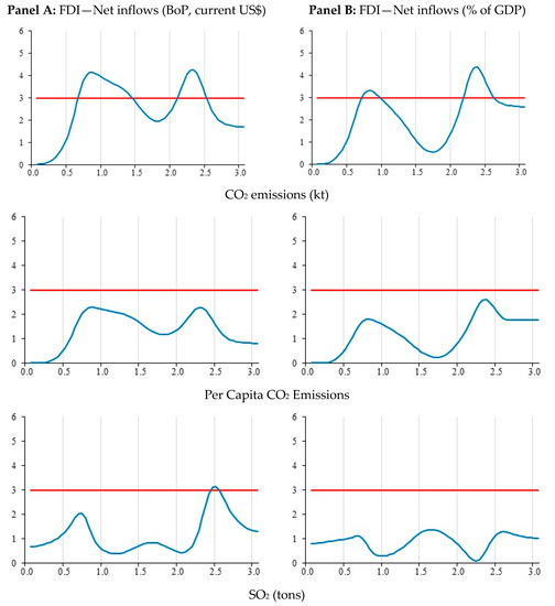
Figure 10.
Short Run and Long Run Causality Test in Frequency Domain from FDI to Emissions. Note: The frequencies (omega) are on x-axis and y-axis show the F statistics testing the null hypothesis of no Granger-causality. The horizontal red line indicates the 5% critical values.
FDI does not cause per capita CO2 emission in short and long runs. This result also holds for when FDI is taken as share of GDP. FDI has no effect on SO2 in the long term and has little effect in the short term. FDI (% of GDP) has no effect on SO2 in short and long terms.
6. Conclusions
The paper explores the effect of FDI on pollution in China using data for the period 1982 to 2016 by applying the wavelet tool. The main findings reveal that FDI positively drives the pollution at high and low frequencies, which confirms the ‘pollution haven hypothesis’ for short and long terms. At low frequency, FDI provoked pollution during the 1980s in the wake of economic reforms when FDI inflows started to increase, and after 2000 due to a surge in FDI and high economic growth which increased production after the joining of WTO by China in 2001. It accelerated the FDI flows of dirty industries and led to both scale and composition effects. Hence, for the short and long term, lax environment regulations have stimulated FDI in polluting industries. Interestingly, FDI has no effect on pollution at medium frequency. These results support the findings of some previous studies showing that FDI increases pollution in China [4,12,51,58]. For robustness analysis, spectral causality analysis was conducted and the results of this spectral causality test indicate that FDI causes CO2 emissions both in the short-run and long-run. It suggests that FDI predicts CO2 emissions in China.
The study has some important policy implications. The government should introduce strict environmental regulations to restrict the entry of pollution industries in the country. The government should also introduce rules so that local firms receiving FDI may adopt and exchange green technology. These measures will help reduce pollution in the country. Further, government should promote education, which will help to reduce pollution. Government should provide incentives to local firms to increase research and development (R&D) investment; it will strengthen the technical efficiency of the host economy, which will lower pollution in China.
Author Contributions
All authors contributed to data collection, estimation, writing and editing of this study. The idea, initial work and data collection are carried out by M.Z. and H.M. The analysis and supportive work is done by S.J.H.S. Critical review and amendments in the draft from W.J. significantly improved the quality of the study.
Funding
This research received no external funding.
Conflicts of Interest
The authors declare no conflicts of interest.
References
- Copeland, B.R.; Taylor, M.S. North-South Trade and the Environment. Q. J. Econ. 1994, 109, 755–787. [Google Scholar] [CrossRef]
- Tobey, J.A. Effects of Domestic Environmental Policy on Patterns of International Trade: An Empirical Test. Kyklos Int. Rev. Soc. Sci. 1990, 43, 191–2019. [Google Scholar]
- Cole, M.A. Trade, the pollution haven hypothesis and the environmental Kuznets curve: Examining the linkages. Ecol. Econ. 2004, 48, 71–81. [Google Scholar] [CrossRef]
- He, J. Pollution haven hypothesis and environmental impacts of foreign direct investment: The case of industrial emission of sulfur dioxide (SO2) in Chinese provinces. Ecol. Econ. 2006, 60, 228–245. [Google Scholar] [CrossRef]
- Kivyiro, P.; Arminen, H. Carbon dioxide emissions, energy consumption, economic growth, and foreign direct investment: Causality analysis for Sub-Saharan Africa. Energy 2014, 74, 595–606. [Google Scholar] [CrossRef]
- Lan, J.; Kakinaka, M.; Huang, X. Foreign Direct Investment, Human Capital and Environmental Pollution in China. Environ. Resour. Econ. 2012, 51, 255–275. [Google Scholar] [CrossRef]
- Levinson, A.; Taylor, M.S. Unmasking the Pollution Haven Effect. Int. Econ. Rev. 2008, 49, 223–254. [Google Scholar] [CrossRef]
- Omri, A.; Nguyen, D.K.; Rault, C. Causal interactions between CO2 emissions, FDI, and economic growth: Evidence from dynamic simultaneous-equation models. Econ. Model. 2014, 42, 382–389. [Google Scholar] [CrossRef]
- Shahbaz, M.; Nasreen, S.; Abbas, F.; Anis, O. Does foreign direct investment impede environmental quality in high-, middle- and low-income countries? Energy Econ. 2015, 51, 275–287. [Google Scholar] [CrossRef]
- Tang, C.F.; Tan, B.W. The impact of energy consumption, income and foreign direct investment on carbon dioxide emissions in Vietnam. Energy 2015, 79, 447–454. [Google Scholar] [CrossRef]
- Wang, D.T.; Chen, W.Y. Foreign direct investment, institutional development, and environmental externalities: Evidence from China. J. Environ. Manag. 2014, 135, 81–90. [Google Scholar] [CrossRef] [PubMed]
- Zhang, Y.J. The impact of financial development on carbon emissions: An empirical analysis in China. Energy Policy 2011, 39, 2197–2203. [Google Scholar] [CrossRef]
- Bin, S.; Yue, L. Impact of foreign direct investment on china’s environment: An empirical study based on industrial panel data. Soc. Sci. China 2012, 33, 89–107. [Google Scholar] [CrossRef]
- Javorcik, B.S.; Wei, S.-J. Pollution havens and foreign direct investment: Dirty secret or popular myth? Contrib. Econ. Anal. Policy 2004, 3, 1–32. [Google Scholar] [CrossRef]
- Antweiler, W.; Copeland, B.R.; Taylor, S. Is free trade good for the environnement. Am. Econ. Rev. 2001, 91, 807–908. [Google Scholar] [CrossRef]
- Eskeland, G.S.; Harrison, A.E. Moving to greener pastures? Multinationals and the pollution haven hypothesis. J. Dev. Econ. 2003, 70, 1–23. [Google Scholar] [CrossRef]
- Grossman, G.M.; Krueger, A.B. Environmental Impacts of a North American Free Trade Agreement; NBER Working Paper No. 3914; MIT Press: Cambridge, MA, USA, 1991; pp. 1–57. [Google Scholar]
- Araya, M. FDI and the environment: What empirical evidence does—And does not—Tell us. In International Investment for Sustainable Development Balancing Rights and Rewards; Routledge: London, UK, 2012; pp. 46–73. [Google Scholar]
- Zhu, Q.; Sarkis, J.; Lai, K.H. Initiatives and outcomes of green supply chain management implementation by Chinese manufacturers. J. Environ. Manag. 2007, 85, 179–189. [Google Scholar] [CrossRef] [PubMed]
- Al-mulali, U. Factors affecting CO2 emission in the Middle East: A panel data analysis. Energy 2012, 44, 564–569. [Google Scholar] [CrossRef]
- Cole, M.A.; Elliott, R.J.R. FDI and the capital intensity of “dirty” sectors: A missing piece of the pollution haven puzzle. Rev. Dev. Econ. 2005, 9, 530–548. [Google Scholar] [CrossRef]
- Al-mulali, U.; Tang, C.F. Investigating the validity of pollution haven hypothesis in the gulf cooperation council (GCC) countries. Energy Policy 2013, 60, 813–819. [Google Scholar] [CrossRef]
- Tamazian, A.; Chousa, J.P.; Vadlamannati, K.C. Does higher economic and financial development lead to environmental degradation: Evidence from BRIC countries. Energy Policy 2009, 37, 246–253. [Google Scholar] [CrossRef]
- Zhang, C.; Zhou, X. Does foreign direct investment lead to lower CO2 emissions? Evidence from a regional analysis in China. Renew. Sustain. Energy Rev. 2016, 58, 943–951. [Google Scholar] [CrossRef]
- UNCTAD. World Investment Report; United Nations Conference on Trade and Development: Geneva, Switzerland, 2018. [Google Scholar]
- Li, M.; Zhang, L. Haze in China: Current and future challenges. Environ. Pollut. 2014, 189, 85–86. [Google Scholar] [CrossRef] [PubMed]
- Liu, Q.; Wang, Q. How China achieved its 11th Five-Year Plan emissions reduction target: A structural decomposition analysis of industrial SO2 and chemical oxygen demand. Sci. Total. Environ. 2017, 574, 1104–1116. [Google Scholar] [CrossRef] [PubMed]
- Acharyya, J. FDI, Growth and the environment: Evidence from India on co2 emission during the last two decades. J. Econ. Dev. 2009, 34, 43–58. [Google Scholar]
- Akbostanci, E.; Tunç, G.I.; Türüt-Aşik, S. Pollution haven hypothesis and the role of dirty industries in Turkey’s exports. Environ. Dev. Econ. 2007, 12, 297–322. [Google Scholar] [CrossRef]
- Baek, J.; Cho, Y.; Koo, W.W. The environmental consequences of globalization: A country-specific time-series analysis. Ecol. Econ. 2009, 68, 2255–2264. [Google Scholar] [CrossRef]
- Chung, S. Environmental regulation and foreign direct investment: Evidence from South Korea. J. Dev. Econ. 2014, 108, 222–236. [Google Scholar] [CrossRef]
- Hitam, M.B.; Borhan, H.B. FDI, Growth and the Environment: Impact on Quality of Life in Malaysia. Procedia Soc. Behav. Sci. 2012, 50, 333–342. [Google Scholar] [CrossRef]
- List, J.A.; Co, C.Y. The effects of environmental regulations on foreign direct investment. J. Environ. Econ. Manag. 2000, 40, 1–20. [Google Scholar] [CrossRef]
- Pao, H.T.; Tsai, C.M. Multivariate Granger causality between CO2 emissions, energy consumption, FDI (foreign direct investment) and GDP (gross domestic product): Evidence from a panel of BRIC (Brazil, Russian Federation, India, and China) countries. Energy 2011, 36, 685–693. [Google Scholar] [CrossRef]
- Smarzynska, B.K.; Wei, S. Pollution Havens and Foreign Direct Investment: Dirty Secret or Popular Myth? National Bureau of Economic Research: Cambridge, MA, USA, 2001. [Google Scholar]
- Xing, Y.; Kolstad, C.D. Do lax environmental regulations attract foreign investment? Environ. Resour. Econ. 2002, 21, 1–22. [Google Scholar] [CrossRef]
- Zeng, D.Z.; Zhao, L. Pollution havens and industrial agglomeration. J. Environ. Econ. Manag. 2009, 58, 141–153. [Google Scholar] [CrossRef]
- Zhang, J.; Fu, X. Do Intra-Country Pollution Havens Exist? FDI and Environmental Regulations in China; SLPTMD Working Paper Series No. 013; Department of International Development, University of Oxford: Oxford, UK, 2008. [Google Scholar]
- Lee, C.G. Foreign direct investment, pollution and economic growth: Evidence from Malaysia. Appl. Econ. 2009, 41, 1709–1716. [Google Scholar] [CrossRef]
- Liang, F.H. Does Foreign Direct Investment Harm the Host Country’s Environment? Evidence from China. 2008. Available online: https://ssrn.com/abstract=1479864 (accessed on 9 July 2018).
- Merican, Y.; Yusop, Z.; Mohd Noor, Z.; Siong Hook, L. Foreign direct investment and the pollution in Five ASEAN nations. Int. J. Econ. Manag. 2007, 1, 245–261. [Google Scholar]
- Sbia, R.; Shahbaz, M.; Hamdi, H. A contribution of foreign direct investment, clean energy, trade openness, carbon emissions and economic growth to energy demand in UAE. Econ. Model. 2014, 36, 191–197. [Google Scholar] [CrossRef]
- Hoffmann, R.; Lee, C.; Ramasamy, B.; Yeung, M. FDI and pollution: A granger causality test using panel data. J. Int. Dev. 2005, 17, 311–317. [Google Scholar] [CrossRef]
- Kim, M.H.; Adilov, N. The lesser of two evils: An empirical investigation of foreign direct investment-pollution tradeoff. Appl. Econ. 2012, 44, 2597–2606. [Google Scholar] [CrossRef]
- Sung, B.; Song, W.Y.; Park, S.-D. How foreign direct investment affects CO2 emission levels in the Chinese manufacturing industry: Evidence from panel data. Econ. Syst. 2018, 42, 320–331. [Google Scholar] [CrossRef]
- Liu, Q.; Wang, S.; Zhang, W.; Zhan, D.; Li, J. Does foreign direct investment affect environmental pollution in China’s cities? A spatial econometric perspective. Sci. Total Environ. 2018, 613–614, 521–529. [Google Scholar] [CrossRef] [PubMed]
- Yang, J.; Wang, Y. FDI and Environmental Pollution Nexus in China. Master’s Thesis, Lund University, Lund, Sweden, 2016; pp. 1–47. [Google Scholar]
- Zheng, J.; Sheng, P. The Impact of Foreign Direct Investment (FDI) on the Environment: Market Perspectives and Evidence from China. Economies 2017, 5, 8. [Google Scholar] [CrossRef]
- Huang, J.; Chen, X.; Huang, B.; Yang, X. Economic and environmental impacts of foreign direct investment in China: A spatial spillover analysis. China Econ. Rev. 2017, 45, 289–309. [Google Scholar] [CrossRef]
- Dean, J.; Mary, L.; Wang, H. Are foreign investors attracted to weak environmental regulations? Evaluating the evidence from China. J. Dev. Econ. 2009, 90, 1–13. [Google Scholar] [CrossRef]
- Haisheng, Y.; Jia, J.; Yongzhang, Z.; Shugong, W. The impact on environmental kuznets curve by trade and foreign direct investment in China. Chin. J. Popul. Resour. Environ. 2005, 3, 14–19. [Google Scholar] [CrossRef]
- Zeng, K.; Eastin, J. International Economic Integration and Environmental Protection: The Case of China. Int. Stud. Q. 2007, 51, 971–995. [Google Scholar] [CrossRef]
- Zheng, S.; Kahn, M.E.; Liu, H. Regional Science and Urban Economics Towards a system of open cities in China: Home prices, FDI flows and air quality in 35 major cities. Reg. Sci. Urban Econ. 2010, 40, 1–10. [Google Scholar] [CrossRef]
- Kirkulak, B.; Qiu, B.; Yin, W. The impact of FDI on air quality: Evidence from China. J. Chin. Econ. Foreign Trade Stud. 2011, 4, 81–98. [Google Scholar] [CrossRef]
- Bao, Q.; Chen, Y.; Song, L. Foreign direct investment and environmental pollution in China: A simultaneous equations estimation. Environ. Dev. Econ. 2011, 16, 71–92. [Google Scholar] [CrossRef]
- Cole, M.A.; Elliott, R.J.R.; Zhang, J. Growth, foreign direct investment, and the environment: Evidence from chinese cities. J. Reg. Sci. 2011, 51, 121–138. [Google Scholar] [CrossRef]
- Chang, N. The empirical relationship between openness and environmental pollution in China. J. Environ. Plan. Manag. 2012, 55, 783–796. [Google Scholar] [CrossRef]
- Jiang, Y. Foreign direct investment, pollution, and the environmental quality: A model with empirical evidence from the Chinese regions. Int. Trade J. 2015, 29, 212–227. [Google Scholar] [CrossRef]
- Aguiar-Conraria, L.; Azevedo, N.; Soares, M.J. Using wavelets to decompose the time-frequency effects of monetary policy. Phys. A Stat. Mech. Appl. 2008, 387, 2863–2878. [Google Scholar] [CrossRef]
- Rua, A. Worldwide synchronization since the nineteenth century: A wavelet-based view. Appl. Econ. Lett. 2013, 20, 773–776. [Google Scholar] [CrossRef]
- Olayeni, O.R. Causality in Continuous Wavelet Transform Without Spectral Matrix Factorization: Theory and Application. Comput. Econ. 2016, 47, 321–340. [Google Scholar] [CrossRef]
- Lee, J.W. The contribution of foreign direct investment to clean energy use, carbon emissions and economic growth. Energy Policy 2013, 55, 483–489. [Google Scholar] [CrossRef]
- Cole, M.A.; Elliott, R.J.R.; Okubo, T.; Zhou, Y. The carbon dioxide emissions of firms: A spatial analysis. J. Environ. Econ. Manag. 2013, 65, 290–309. [Google Scholar] [CrossRef]
- Boashash, B. Time-Frequency Signal Analysis and Processing, 2nd ed.; Academic Press: Cambridge, MA, USA, 2015. [Google Scholar]
- Crowley, P.M.; Mayes, D.G. How fused is the euro area core? An evaluation of growth cycle co-movement and synchronization using wavelet analysis. OECD J. J. Bus. Cycle Meas. Anal. 2008, 4, 63–95. [Google Scholar]
- Hallett, A.H.; Richter, C. Have the Eurozone economies converged on a common European cycle? Int. Econ. Econ. Policy 2008, 5, 71–101. [Google Scholar] [CrossRef]
- Breitung, J.; Candelon, B. Testing for short- and long-run causality: A frequency-domain approach. J. Econ. 2006, 132, 363–378. [Google Scholar] [CrossRef]
- Bouri, E.; Roubaud, D.; Jammazi, R.; Assaf, A. Uncovering frequency domain causality between gold and the stock markets of China and India: Evidence from implied volatility indices. Financ. Res. Lett. 2017, 23, 23–30. [Google Scholar] [CrossRef]


© 2018 by the authors. Licensee MDPI, Basel, Switzerland. This article is an open access article distributed under the terms and conditions of the Creative Commons Attribution (CC BY) license (http://creativecommons.org/licenses/by/4.0/).