Sustainable Decision Making for Store Brand Product

Abstract

We investigate a multi-brands sustainable channel coordination problem where a national brand manufacturer sells a product through two local retailers competing against their own store brand product, respectively. We shows how the retailers strategically optimize the price and quality of private brands given the customer tastes and the production costs of the store brands in order to make their store brands sustainable. We identify two underlying strategic forces; a competitive force, and a quality force. First, we find that retailers have an incentive to position their store brand far away from the national brand in order to maximize monopolistic power. This strategic force attenuate the incentives for customer to switch to other retailer’s store brands. One the other hand, we show that the retailers prefer increasing the store brand’s quality to get more profit margin when the production cost is relatively high as well.

1. Introduction

Selling store brand products along with the national brand products on the same shelves in a grocery store or supermarket have been becoming popular in retailer markets over the past two decades. Walmart have ‘Great Value’ for sliced bread, frozen vegetables, frozen dinners, light bulbs, cinnamon rolls, and canned food. Another store brand for consumable pharmacy and health and beauty product category, ‘Equate’ is very popular example of multivitamin over-the-counter medicine competing with the ‘Centrum’, the national brand product and the market leader. Costco carry Kirkland brand for cheaper and lower quality of product such as bottled water, cereal, and nuts. Some of above listed store brand products are targeting less-for-more segments of the consumer groups; however, some of them are positioning as close to the national brand product as possible. They used to be considered as cheap products or simple generic products in the past as price-sensitive customers could substitute the national brands with them. However, a recent report shows that the market share of store brands in the United States was about 18 percent in 2013 [1]. This report also states that 33 percent of North American consumers have come to the realization that, in terms of quality and value, store brand products are equally as good as the national brands they used to purchase. In fact, store brands today are carefully managed and marketed in order to improve the retailer’s competitive edge. Therefore, many are actually seen as brands in their own right.

Based on such trend in retailer market such as grocery market, researches have been conducting actively in the areas of store brands. Initial studies have found that a retailer’s introduction of a store brand product can be viewed as its resource use for additional marketing strategies such as store differentiation, store loyalty, or store profitability. More recently, studies have shown that retailers who offer store brands set a quality of their store brands very close to the quality of leading national brands in terms of product characteristics because of its strategic relationship with the national brand [2,3,4,5,6]. Retailers have to make two positioning decisions, namely, horizontal and vertical positioning. The horizontal positioning of a product, for example, can be a decision on product design, such as color, size, shape, and package, whereas vertical positioning mostly refers to the decision on product quality, which is measured as a relative quality level to the national brand.

Even though an overwhelming studies have been conducted over the last two decades, with authors’ best knowledge, only a few of the following studies have addressed a retail-level competitive environment [7,8,9,10,11]. These studies suggest that retailers introduce quality-equivalent store brands and focus on competitive strategies involving which brand the retailers advertise or whether a store brand is introduced. These strategies can also show why retailers have an incentive to introduce store brands if the levels of competition between the retailers vary under a certain consumer structure. What previous studies minimally focused on, however, is the fact that consumers who are willing to pay less are non-brand seekers, and thus, they tend to purchase a store brand in a retailer who is more likely to buy another store brand from different retailers.

In the current study, we argue that the competitor of a retailer, who focuses on the common consumer segment, may be other retailers who provide their own store brands, rather than the national brand that they have on stock. A separate segment whose consumers are loyal to the national brand usually exists, and they are not considered as they easily switch loyalty to store brands only because of product prices. Therefore, this study focuses on investigating how a retailer can sustain their store brand products’ quality and price under a competitive setting. To this extent, the market we investigate is in the form of a monopolistic competition. (Products are differentiated in terms of customer segments’ tastes. Given that, the market we design in this study can be interpreted as a market with bilateral monopolists even though each retailer sells a common national brand manufacturer’s product.) Two retailers with substitutable store brand products face each other as they compete with a common national brand product.

We argue that retailers vertically position their store brands very close to the national brand because of (a) their competitive reaction toward the national brands and/or (b) their strategic decision against the other retailers that offer store brands. Therefore, we consider a monopolistically competing market where a retailer competes with the competing retailer’s both the store brand and the national brand. Furthermore, we investigate two segments of consumers: (a) one includes those who are more localized to one retailer; and (b) the other involves another set of localized consumers for the other store. Based on this structure, we address the following two main research questions. First, how does a retailer position its own store brand (i.e., product quality) and set a product price? Second, how are these decisions affected when store-level competition becomes more (or less) localized?

The rest of the paper is organized as follows: Section 2 reviews the existing literatures, whereas the model is introduced in Section 3. In Section 4, we analyze the market of two localized retailers that share one common manufacturer and then compare the interactions on decision-making of market players. Finally, we conclude and discuss future research in Section 5. The derivations and proofs are given in the Appendix A.

2. Literature Review

Initial literature stream of store brands focus mainly on the existence of store brands validity and profitability of their introduction. The work done by Raju, Sethuraman, and Dhar (1995) is one of the studies that initiated such research stream [12]. They analyze a grocery market including bakery and deli products and frozen goods product categories that consists of three players: two manufacturers selling a national brand and a common retailer who introduces a store brand. Raju et al. (1995) solve for equilibrium solutions using a linear demand system and show the tendency of store brands to increase the retailer’s category profit when the cross-price sensitivity among national brands is low and the cross-price sensitivity between the national brands and the store brand is high [12]. Some other works also explain what role store brands can play as a leveraging effect [13,14,15]. Mills (1995) shows that private label marketing generates stronger power of the retailer’s position via a national brand manufacturer. Narasimhan and Wilcox (1998) argue that a store brand can use bargaining power toward the national brand, and thus lead a higher store brand margin. There are also some early works that examine store brands from different angles. Both of Hoch and Banerji (1993) illustrated that market share of private labels or store brands varies across supermarket merchandise group, for example, 65% of sales of frozen green beans are covered by store brands or private labels, and however, only 1.1% of sales of personal deodorants are store brands [16]. Using data from 34 food categories for 106 supermarket stores in the largest 50 retail markets in the United States, Dhar and Hoch (1997) empirically conduct a cross-category analysis and a cross-retailer analysis, respectively, to find conditions for successful store brands business [17]. Their within-category across-retailer analysis demonstrates that the national brand-private label price differential exerts an important positive influence on store brand performance. Other empirical approaches have also made and contributed in analyzing margins and profits from store brands compared to those from national brands [18,19,20,21,22].

More recent studies on store brands address quality problems (i.e., positioning). Sayman, Hoch and Raju (2002) demonstrate that the most profitable strategy for the retailer is to position the store brand close to the high tier national brand [2]. Using a Nash bargaining game for the demand model, Morton and Zettlemeyer (2004) replicated Sayman’s research, wherein they positioned private brands as close to the leading national brand as possible [3]. Du, Lee, and Stalin (2005) found that three possible strategies for each parameter space are optima; (i) close to the top tier national brand; (ii) close to the lower tier national brand; or (iii) around midpoint between the two national brands [23]. Choi and Coughlan (2006) reported similar results by using the representative consumer approach [4]. In addition, Soberman and Parker (2006) and Gabrielsen and Sorgard (2007) argue that high quality store brands can be used as a price discrimination tool for the retailer [24,25]. Although these studies have focused on the system characterized by two manufacturers and a common retailer, we developed our model based on a situation with one manufacturer and two retailers, who can introduce their own private brand by choosing the vertical and horizontal positions.

Our research is also closely related to topics of product line rivalry and market segmentation [26,27]. These topics have been being popular, especially in marketing area and have been widely studied with different setups and dimensions in other business areas and economics. Katz (1984) introduces game theories to play product positioning games by considering horizontal and vertical differentiation [28]. Gilbert and Matutes (1993) studies a product line strategy with exogenous quality levels and proves that firms prefer a full product lines when a differentiation among firms is sufficiently large [29]. Villas-Boas (1998) solves channel issues and proves how manufacturers increases its profits over retailers by differentiating its product with quality [30]. Villas-Boas and Schmidt-Mohr (2008) extend this result by applying it to a credit market [31]. They claim that a higher level of differentiation will make firms to compete less intensively for high profitable consumers.

Desai (2001) investigates multiproduct firms bearing with a cannibalization problem in designing their product lines [32]. Desai (2001) develops a model of a market characterized by both quality and taste differentiation just like the current study sets up, but he uses Hotelling (1929) model for horizontal differentiation while the current study uses a utility function that is suggested by Du, Lee, and Stalin (2005) to describe two levels of market segmentations [23,33]. Also, Desai (2001) suggests that an intense competition in the low-valuation segment affects the market, which is also one of our main questions in this study [32]. Villas-Boas and Schmidt-Mohr (2008) and Kim and Choi (2017) later support this argument by showing that high degree of differentiation pools customer types for high and low segments [31,34,35,36,37]. In sum, although product line problems do not directly propose a solution for channel-structured problems, their optima decisions suggests valuable insights to reflect the problem of store brands in terms of strategic decision on product positioning.

3. Model

As an analytical analysis, we start with the parsimonious model that only has essential variables to design the mathematical model to test. Thus, we intentionally reduce the dimension of the analysis in order to extract solid dynamics between independent variables (i.e., decision variables, or choice variables) and dependent variables such as sales or profit. Unlike other methodologies such as empirical research using real world data sample which can be influenced by lots of factors, in analytical modeling research, by soling a few key independent variables, we are more likely to focus on concrete direct and indirect effects of parameters on dependent variables. Adding one more dimension (e.g., putting one additional choice variables) often drives the whole problem to be extremely hard to solve mathematically, and thus ends up giving us ambiguous insights.

We assumed in this particular project that quality level and price are the two most important variables when customers are shopping at local supermarkets or other various types of grocery stores or wholesalers. Any daily product such as a toothbrush or a can of soda might be the good example of this behavior. As far as a customer does not distinguish the taste of a store brand drink from that of a national brand, that is, if two products’ quality difference is minimal to the customer, she/he would buy a store brand by paying less. However, if a customer can easily find a quality difference between a store brand and a national brand, then which product variant this customer buys is dependent upon how much a customer is price-sensitive. However, this price-sensitivity is even a heterogeneous factor across customers. On the contrary, from the store brand producer’s point of view, retailers can decide the quality level of their own product given the quality of national brands and/or customer’s willingness-to-pay.

What we try to answer in this study is a strategic decision that a retailer should make; i.e., how much to price and what quality of product to produce in order to achieve retailer’s profit maximization. A retailer carefully investigates customers’ preference (i.e., heterogeneity) and price sensitivity (i.e., willingness-to-pay) and make a decision for two variables; price and quality level of the store brand product, by knowing the current quality level and price of national brands. In sum, in the customers’ mind, there must be many determinants that prompt their decisions when they purchase an item. These determinants may be not only price or quality, but also brand perception or loyalty or even location of the stores. Facing with all the situations of an academic research that uses one methodology, our study must have a limitation, and the results driven by our model setup are not able to incorporate all valuable dimensions. However, our model clearly gives us answers to questions we would like to solve based on the model setup. Those are answers of effects of retailers’ strategic decisions because price and quality are set in ways of maximizing profits and utilities.

3.1. Consumer Utilities and Market Structure

We consider a market that consists of one manufacturer and two competing retailers with their store brand products, SA and SB, respectively. Furthermore, consider a manufacturer who produces a national brand and sells it through both retailers. We assume that two segments of consumers exist. Within each segment, consumers are heterogeneous with respect to product valuation (or equivalently, willingness to pay), ${\theta }_i$, which is uniformly distributed between 0 and 1 with a density of 1.

This study models consumer behavior based on the utility function suggested by Du, Lee, and Staelin (2005; DLS hereafter) [23]. We consider both vertical and horizontal heterogeneities of consumers for their utility function. The utility function is given below:

$$U_{ij}={\theta }_i{v}_j-t_i\left|x_i-x_j\right|-p_j$$

(1)

where ${\theta }_i$ is the willingness of consumer segment i to pay for quality, $v_j$ is the quality level ($j=NA,NB,SA,SB$) of seller j, $t_i$ is the mismatching cost of consumer i, $\left|x_i-x_j\right|$ measures the disutility between consumer i’s ideal point and brand j’s position, and $p_j$ is the retail price of brand j.

This part discusses three things: (1) the heterogeneous parameters and their correlation; (2) the rescaling of degree of product mismatch based on the correlation of the parameters; and (3) the new utility functions converted to better fit our model. First, the above equation indicates that consumers are heterogeneous in three manners: willingness to pay for quality (${\theta }_i$), cost of mismatch ($t_i$) and degree of product mismatch ($x_i-x_j$). Moreover, we consider different mismatching transportation costs, in which higher transportation costs are equivalent to lower price sensitivity. Thus, given $t_H>t_L$, high-type customers respond less to price changes than low-type ones. We also assume that ${\theta }_H>{\theta }_L$, which means that the willingness-to-pay increases as the quality level increases. Thus, as Desai (2001) showed, we assume that if ${\theta }_H>{\theta }_L$, then, $t_H\ge t_L$; that is, ${\theta }_i$ and $t_i$ are positively correlated [33].

Following DLS, we define a rescaled mismatch variable, $m_{ij}=\left|x_i-x_j\right|/b$ where b is the constant that perfectly maps $t_i$ into ${\theta }_i$, i.e., ${\theta }_i=b{t}_i$. Therefore, the utility function is rewritten as

$$U_{ij}={\theta }_i\left(v_j-m_{ij}\right)-p_j$$

(2)

We assume that each customer segment is targeted by one store brand and the brand characteristics fit the taste of its target segment perfectly. Let d denote the “perceived distance” between two store brand locations. The positions of the store brands in relation to the national brand are captured by $x_j$. Hence, $x_{j}d$ and $\left(1-x_j\right)d$ capture the distances from each of the positions of store brand j ($x_{SA}$ and $x_{SB}$), respectively, toward a common location of the national brand ($x_N$). See Figure 1.

We also set the quality levels of the national brand, retailers A and B as one, $q_{SA}$, and $q_{SB}$, respectively ($0<q_{SA,}{q}_{SB}\le 1$). For now, we assume that the quality level of the national brand reaches the maximum level of one. Therefore, based on assumptions stated above, the utility functions of consumer i in segment A for manufacturers and retailers can be summarized as follows:

$$U_{i,NA}={\theta }_i\left(1-\frac{d}{2}\right)-p_{NA}$$

(3)

$$U_{i,SA}={\theta }_i\left(q_{SA}\right)-p_{SA}$$

(4)

$$U_{i,SB}={\theta }_i\left(q_{SB}-d\right)-p_{SB}$$

(5)

Similarly, consumer i in segment B has the following utility functions for one manufacturer and two retailers:

$$U_{i,NB}={\theta }_i\left(1-\left(d-\frac{d}{2}\right)\right)-p_{NB}$$

(6)

$$U_{i,SA}={\theta }_i\left(q_{SA}-d\right)-p_{SA}$$

(7)

$$U_{i,SB}={\theta }_i\left(q_{SB}\right)-p_{SB}$$

(8)

Please note that when ${\theta }_i$ is close to zero, the net utility of consumer i depends mostly on prices and minimally on the quality levels and positions of the products; furthermore, it indicates high price sensitivity and low brand loyalty.

3.2. Derivation of Demand

The market demand for each brand can be derived from Equations (3)–(8). Please note that given our interest in finding the effects of the characteristics of store brands on the market, we assume that retailers constantly offer store brands. Thus, a retailer’s introduction of a store brand is not deemed as a strategic decision in this study. In addition, we will also derive and discuss a condition to the extent in which introducing a store brand is not a profitable decision. Moreover, without loss of generality, the location of the national brand is assumed at half of the distance between two store brands. Thus, $x_{N}d=d/2$.

We determine the rank order of the three brands in terms of gross utility for each segment. In each segment i, there is a marginal consumer who is indifferent to purchasing between national brand or a store brand and between a store brand and another store brand. For example, in Segment A, a consumer of the first case can be identified by equating Equations (3) and (4). That is, $U_{i,NA}={\theta }_i\left(1-\frac{d}{2}\right)-p_{NA}$ and $U_{i,SA}={\theta }_i\left(q_{SA}\right)-p_{SA}$. Solving them for ${\theta }_i$, ${\theta }_{A,NASA}=\frac{2\left(p_{NA}-p_{SA}\right)}{2\left(1-q_{SA}\right)-d}$, where the first subscript denotes the segment and the second one (NASA) represents the two brands being compared. Thus, NA is the (common) national brand being sold at the physical store location of the retailer and SA is the retailer’s store brand. In a same fashion, we can obtain ${\theta }_{A,SASB}=\frac{p_{SA}-p_{SB}}{d+q_{SA}-q_{SB}}$ for an indifferent consumer between purchasing a store brand and the other store brand. In this manner, we determine the four critical $\theta$’s for each of segment i = A, B, labeled as ${\theta }_{A,NANB}$ ${\theta }_{A,NASA}$, ${\theta }_{A,NASB}$, and ${\theta }_{A,SASB}$ for segment A, and ${\theta }_{B,NBNA}$, ${\theta }_{B,NBSB}$, ${\theta }_{B,NBSA}$, and ${\theta }_{B,SBSA}$ for segment B. We determine the within-segment demand for each brand by partitioning the unit line representing each segment as shown in Figure 1.

Let H, M, and L as symbols for the three ranking levels; that is, they represent the brands of highest, medium, and lowest rankings, respectively. For example, if buying a national brand has consumers with the highest utility compared to buying the other two (store brands); thus, it will be placed in the highest ranking and take the portion of the highest part of the vertical line segment. For example, if buying store brand B shows the lowest utility in Segment A, then the corresponding portion will be the lowest part of the vertical line. We assume a full covered-market, wherein each vertical segment is partitioned by three different brands depending on the ranking discussed here. (See Appendix A for the detailed derivations.) Accordingly, the demand functions for the manufacturer and the retailer in Segment A are, respectively, given by:

$$D_{A,H}=1-Min\left[1,Max\left\{{\theta }_{A,NANB},{\theta }_{A,NASA},{\theta }_{A,NASB},{\theta }_{A,SASB}\right\}\right]$$

(9)

$$D_{A,M}=1-D_{A,H}-Min\left[1-D_{A,H},{\theta }_{A,-H}\right]$$

(10)

$$D_{A,L}=1-D_{A,H}-D_{A,M}$$

(11)

Likewise, we have the demand functions of the manufacturer and the retailer in Segment B as:

$$D_{B,H}=1-Min\left[1,Max\left\{{\theta }_{B,NBNA},{\theta }_{B,NBSB},{\theta }_{B,NBSA},{\theta }_{B,SBSA}\right\}\right]$$

(12)

$$D_{B,M}=1-D_{B,H}-Min\left[1-D_{B,NB},{\theta }_{B,-H}\right]$$

(13)

$$D_{B,L}=1-D_{B,H}-D_{B,M}$$

(14)

3.3. Timing of the Game

The game is played in the following steps:

(1)

Once retailers decide to provide their own store brand, they simultaneously choose qualities of their own store brands given a fixed quality level of the national brand product, which is assumed to be the maximum possible of one unit.

(2)

The manufacturer decides the wholesale price of the national brand product in a way of maximizing its own profit.

(3)

To maximize product category profits, retailers simultaneously set retail prices for both the national and store brands that they carry.

4. Analysis

In this section, we analyze the basic model in a step-by-step fashion and derive insights regarding the impact of retailer competition on the quality of store brands. Our basic model assumes that retailers are symmetric in every aspect because one common manufacturer sells a national brand product through both retailers with the same price.

4.1. Profit Functions of the Manufacturer and the Retailer (When $\overline{d}<d$)

We consider the situation where two retailers have a certain horizontal distance. With a positive d, each retailer can be shown as a bilateral monopolist. However, the existence of the national brand in between the two retailers may not allow them to solely operate in local monopolies. This assumption of a positive d simplifies the model in a plausible range. Considering the location of two retailers at the most preferred positions to each of two consumer segments under our setup of the symmetric retailers, this positive d assumption can play as a boundary condition for each segment only consumed by its own buyers. Thus, in a single segment, we only consider two partitions of consumers who prefer to purchase product from retailers in that particular segment. This is the most profitable case for retailers. For example, consumers in Segment A only consume either national or store brands A under $\overline{d}<d$. If d decreases $\overline{d}$, the consumers in one segment start transferring to the other segment. However, quality is a function of d. Retailers can strategically choose a quality level that prevents customers from brand switching across the segments. Therefore, even if the length of d enlarges, retailers will choose their quality levels in the most profitable manner.

To determine the d-condition, recall the demand derivation described in Section 3.2. Based on the argument above, we derive the condition for d and the demand forms in each segment. Consider segment A. As discussed, this is only partitioned by either the store brand A (SA) or the national brand A (NA): (i) First, compare Equations (3) and (4), $U_{A,NA}={\theta }_A\left(1-\frac{d}{2}\right)-p_{NA}$ and $U_{A,SA}={\theta }_A\left(q_{SA}\right)-p_{SA}$. Considering that Segment A consists of consumers who prefer SA the most, d is determined accordingly to satisfy $U_{A,NA}<U_{A,SA}$. We can easily derive $d\le 2\left(1-q_{SA}\right)$, assuming $p_{NA}\ge p_{SA}$ (No restriction is made such that the price of the national brand has to be greater than or equal to that of the store brand. However, it is reasonable to assume that the national brand whose quality level is assumed to be the maximum high will be priced higher than store brand’s price. If the total valuation from the national brand is higher but its price is lower than those of the store brand, no one will buy the store brand. On the contrary, if the total valuation of the national brand is lower but its price is higher than the store brand’s total valuation and price, no one will buy the national brand. Thus, we exclude such unreasonable situations from our model by making $p_{NA}\ge p_{SA}$). Next, compare $U_{A,NA}={\theta }_A\left(1-\frac{d}{2}\right)-p_{NA}$ and ${\theta }_A\left(q_{SB}-d\right)-p_{SB}$, which drives a condition of $2\left(1-q_{SB}\right)\le d$. From the partitioning results above, we find that the top portion will be consumers of purchasing SA. Then, the next portion of the vertical line will be filled with the NA buyers, and SB-purchasers will be in the third place (the lowest region). However, for SB-purchasers not to be there in segment A, the following condition must be met: ${\theta }_A<\frac{p_{SB}}{\left(q_{SB}-d\right)}$. It implies that $q_{SB}<d$. Therefore, we summarize three d-conditions together as: $2\left(1-q_{SB}\right)\le d\le 2\left(1-q_{SA}\right)$ and $q_{SB}<d$. First inequalities will be almost automatically satisfied under a symmetric setting. The second inequality finally shows how d should be large. Since any q is assumed to be less than 1, we conclude that $0\le q_{SB}\le 1<d$.

If any of inequalities above is not satisfied, consumers will start jumping to the other segments. However, we do not consider such situations in this section. We conclude the demand functions for NA and SA as:

$$D_{A,SA}=1-\frac{2\left(p_{NA}-p_{SA}\right)}{2\left(1-q_{SA}\right)-d}$$

(15)

$$D_{A,NA}=\frac{2\left(p_{NA}-p_{SA}\right)}{2\left(1-q_{SA}\right)-d}$$

(16)

Similarly, the demand functions in Segment B are:

$$D_{B,SB}=1-\frac{2\left(p_{NB}-p_{SB}\right)}{2\left(1-q_{SB}\right)-d}$$

(17)

$$D_{B,NB}=\frac{2\left(p_{NB}-p_{SB}\right)}{2\left(1-q_{SB}\right)-d}$$

(18)

The production cost functions are identical across all firms. The marginal cost of producing a product of quality $q$ is $c\left(q\right)=\frac{\gamma q^2}{2}$, where $\gamma$ is the cost parameter that reflects the relative expense of production. Based on the assumptions and the models derived in the previous section, the objective functions of the manufacturer and the retailer are given by

$${\pi }_N=\left(w_{NA}-\frac{\gamma q_{NA}^2}{2}\right)D_{A,NA}+\left(w_{NB}-\frac{\gamma q_{NB}^2}{2}\right)D_{B,NB}$$

(19)

$${\pi }_{SA}=\left(p_{NA}-w_{NA}\right)D_{A,NA}+\left(p_{SA}-\frac{\gamma q_{SA}^2}{2}\right)D_{A,SA}\mathrm{s}.\mathrm{t}.p_{NA}\ge w_{NA},$$

(20)

$${\pi }_{SB}=\left(p_{NB}-w_{NB}\right)D_{B,NB}+\left(p_{SB}-\frac{\gamma q_{SB}^2}{2}\right)D_{B,SB}\mathrm{s}.\mathrm{t}.p_{NB}\ge w_{NB}.$$

(21)

The constraints in Equations (20) and (21), which play two roles, indicate that the prices of national brands should be greater than or at least equal to the wholesale price. First, this constraint prevents the model from driving into an infeasible solution (e.g., negative price), so that it provides us to have computational convenience to easily capture the correct optimal values. More importantly, this constraint maintains our setup for market structure stability. As we assume that retailers have already decided to produce store brands, this study is not concerned about the factors motivating them to introduce store brands. For instance, we assume that the retailer may introduce a store brand in a particular situation and try to make more profit with a higher store brand margin by setting a negative national brand price. This situation highly motivates the retailer to produce a store brand. However, we would like to exclude such situations here to observe a case where retailers do not manipulate margins, such that their strategic focus is placed only on decisions of prices and qualities.

4.2. Optimal Values

We assume that all the horizontal positions of the manufacturers and the retailers will be exogenously determined. Two competing retailers are assumed to be located at the end points of line d, which we defined as the distance of two segments. However, this is not an assumption made arbitrarily, it is also the most reasonable retailer location because the localized consumer segments match the best when their preferred store brands are at each of their line positions. Furthermore, as mentioned, we assume that the manufacturer is located at the middle point of this distance.

Using multipliers ${\lambda }_A$ and ${\lambda }_B$ for the retailers’ problem, (1) we form the Lagrangian objective functions; (2) differentiate them with respect to $p_j$ ($j=NA,NB,SA,SB$); (3) make them zero ($\frac{\partial L_{SA}}{\partial p_{NA}}=0,\frac{\partial L_{SB}}{\partial p_{NB}}=0,\frac{\partial L_{SA}}{\partial p_{SA}}=0,\frac{\partial L_{SB}}{\partial p_{SB}}=0$); and (4) solve them simultaneously for optimal prices. We then obtain best response retail prices as follows: $i=A,B$,

$${\widehat{p}}_{Ni}\left(w_{Ni}^{\ast },q_{Si}^{\ast }\right)=w_{Ni}^{\ast }\left(q_{Si}^{\ast }\right),$$

(22)

$${\widehat{p}}_{Si}\left(w_{Ni}^{\ast },q_{Si}^{\ast }\right)=\frac{1}{4}\left(-2\left(1-q_{Si}^{\ast }\right)+d+2w_{Ni}^{\ast }+q_{Si}^{\ast }{}^2\right).$$

(23)

Substituting these values into the profit functions of the manufacturers and differentiating them with respect to wholesale prices, we obtain:

$${\widehat{w}}_{Ni}\left(q_{Si}^{\ast }\right)=\frac{\gamma }{2},i=A,B$$

(24)

Now, we plug the wholesale prices along with the best price responses back into the problems of the retailers and the manufacturers, and then differentiate them with respect to qualities resulting in the following quality levels:

$$q_{SA}^{\ast }=q_{SB}^{\ast }=\frac{1-\sqrt{{\left(1-\gamma \right)}^2+d\gamma }}{\gamma }$$

(25)

4.3. Feasibility, Competitive Statics and Discussion

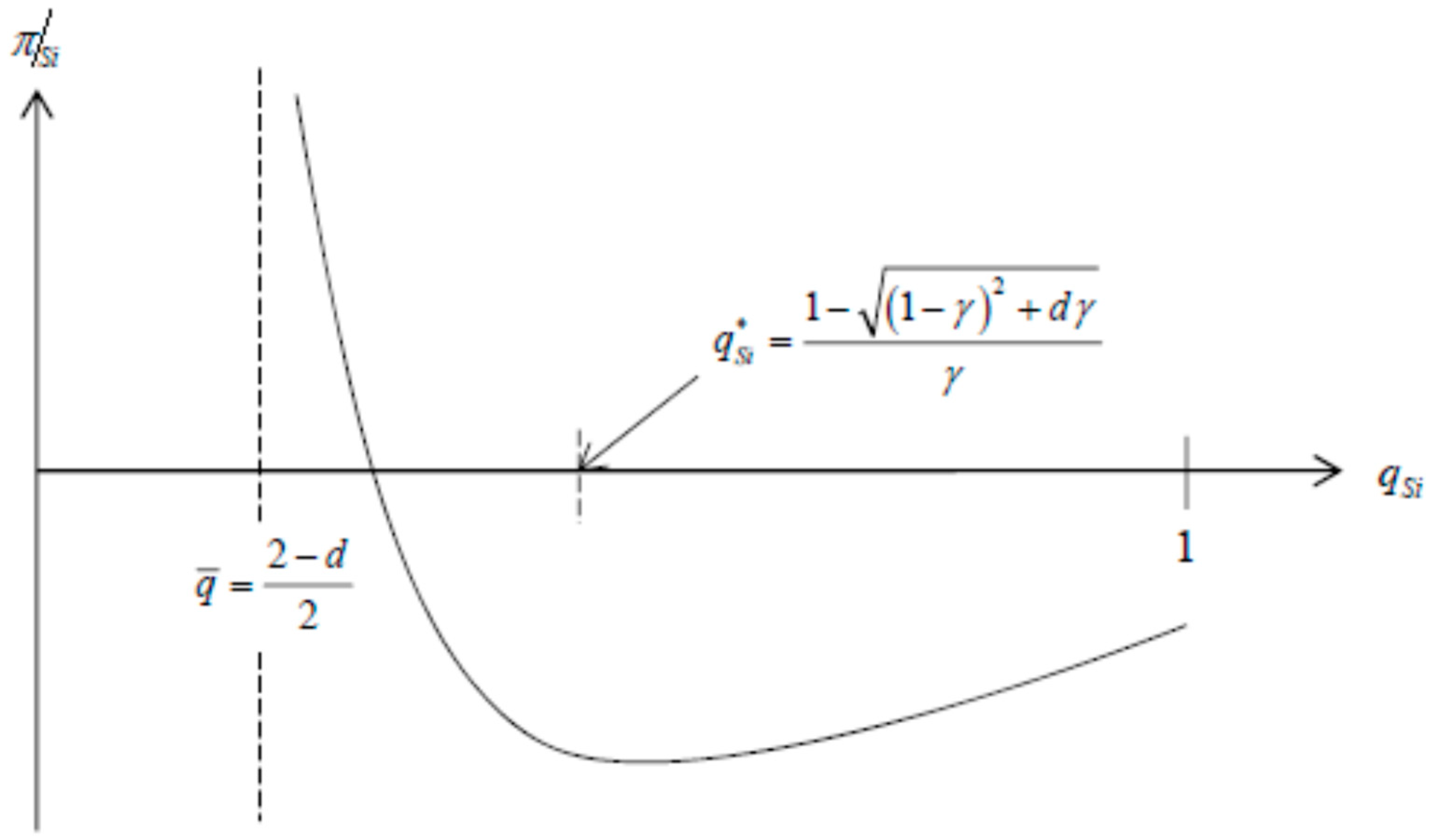
We initially analyze how the retailer determines the level of store brand quality by confirming the quality level obtained in Equation (25). To do so, we should observe the shape of the retailers’ profit functions first given the retail and wholesale prices obtained in the previous section. By plugging the retail and wholesale prices from Equations (22)–(24) into the retailer’s objective function, the retailer’s profit is given by

$${\widehat{\pi }}_{Si}=\frac{{\left(\gamma -q_{Si}^2\gamma -\left(2\left(1-q_{Si}\right)-d\right)\right)}^2}{-8\left(2\left(1-q_{Si}\right)-d\right)}$$

(26)

For the retailer with a positive profit, the above equation should be positive. The numerator is always positive, and the denominator will be positive only if $2\left(1-q_{Si}\right)-d$ is negative. This leads the important feasible condition of $q_{Si}>\frac{2-d}{2}$. Given this, we check the first order conditions to examine how the profit of the retailer is affected by the quality level. The first order condition of Equation (26) is given by

$$\frac{\partial {\widehat{\pi }}_{Si}}{\partial q_{Si}}=\frac{2\left(1-q_{Si}\gamma \right)\left(\gamma -q_{Si}^2\gamma -\left(2\left(1-q_{Si}\right)-d\right)\right)}{4\left(2-2q_{Si}-d\right)}-\frac{{\left(\gamma -q_{Si}^2\gamma -\left(2\left(1-q_{Si}\right)-d\right)\right)}^2}{4{\left(2-2q_{Si}-d\right)}^2}$$

(27)

The sign of this FOC is easy to determine: First, suppose that $\gamma$ is sufficiently large and with the condition found above ($q_{Si}>\frac{2-d}{2}$), we have $\left(1-q_{Si}\gamma \right)>0$, $\left(\gamma -q_{Si}^2\gamma -\left(2\left(1-q_{Si}\right)-d\right)\right)>0$, and $\left(2-2q_{Si}-d\right)<0$. Hence, the first term of LHS is negative. The second term is straightforwardly negative. Therefore, we conclude that ${\frac{\partial {\widehat{\pi }}_{Si}}{\partial q_{Si}}|}_{q_{Si}>\frac{2-d}{2}}<0$. Second, suppose that $\gamma$ is small. Then, ${\frac{\partial {\widehat{\pi }}_{Si}}{\partial q_{Si}}|}_{q_{Si}>\frac{2-d}{2}}<0\mathrm{and}>0$. Given a fixed distance from the other retailer, the profit of a retailer decreases initially as its store brand quality increases. However, at a certain point of quality, the profit increases as the quality level rises. Thus, we summarize our observations as follows:

Proposition 1.

Given a fixed taste distance from its competitor, (i) with a small$\gamma$, the profit of the retailer decreases as its store brand quality increases; (ii) with a large$\gamma$, the profit of the retailer initially decreases as its store brand quality rises. However, at a certain point of quality, the profit starts increasing as the quality level increases.

However, regardless of how large or little $\gamma$ is, the profit of the retailer commonly increases when the quality level decreases. The boundary where the profit stops increasing is at $\frac{2-d}{2}<q_{Si}$. The derivative function of the retailer’s profit consists of two terms as shown in Equation (28). In fact, the second term decreases or increases faster than the first term. Thus, if the quality used in this boundary decreases, the profit dramatically starts increasing. This actually provides us a sign of the maximum profit.

Next, we observe how the quality decisions may be affected by taste distance. We have

$$\frac{\partial q_{Si}}{\partial d}=-\frac{1}{2\sqrt{1+\gamma \left(-2+d+\gamma \right)}}$$

(28)

This is straightforward to conclude that the above equation is always negative. Lemma 1 follows.

Lemma 1.

The store brand quality decreases as the horizontal taste distance between the retailers increases.

From the lemma above and the discussion in Section 4.1, we can observe the relationship between the levels of the localization of retailers and the quality of their store brand and profits ($\frac{\partial {\pi }_{Si}}{\partial d}=\frac{\partial {\pi }_{Si}}{\partial q_{Si}}\cdot \frac{\partial q_{Si}}{\partial d}$). As d increases, the products produced by two retailers are further distinguished, which loosens competitive intensity. On the one hand, an enlarged localization of the retailers leads to a weak competition intensity. The retailers will then have no incentive to raise the quality levels of their store brands as well. On the other hand, if the localization becomes more indifferent, which means that the competition intensifies, the retailers are more likely to increase the store brand quality levels. If the quality increases, depending on the value of $\gamma$, the profit may increase or decrease. However, if the quality decreases, the profit tends to increase at all times. We summarize the following proposition.

Proposition 2.

Given Lemma 2, the boundary of the store brand quality increases when the competition intensity between retailers is high. The profit of the retailers will be globally maximized when its quality is determined close to this lower boundary.

Proof. 

See Appendix A.

The proposition above suggests that the retailer should raise the quality level of its store brand high enough when it strongly competes with other sellers. Afterwards, this quality level becomes a lower boundary of feasible ranges for its profit, and the maximum profit is then achieved at this point. However, it can moderately keep the quality level when the perceived distance of consumers from its competitor is sufficiently far.

Figure 2 illustrates what we found and discussed above. Given an assumption of a fixed production cost, the profits of the retailers increase as the quality of its store brand product either becomes high enough compared to the national brand or low enough toward the feasible lower boundary of a certain quality level. A bilaterally monopolized retailer has two store brand strategies. First, they can try to be less indifferent to each other by offering a relatively higher quality of the store brand product. Second, they can be localized by reducing their store brand quality, through which they can capture a customer segment of their own by considering that they can serve both national and store brands customers in each segment. If a retailer lowers its store brand quality when the distance between two segments becomes closer, the customers of its own segment will start jumping over from one segment to the other segment or vice versa. Moreover, the retailer tends to produce high quality store brand products when the retailer level competition intensifies. By offering a high quality store brand product through decreased localization, it can either earn a higher margin for its own brand and/or compete with the national brand manufacturer more strongly.

5. Conclusions and Future Research

Store brand is not a generic substitute anymore in retailing. Over the past two decades, an introduction of store brands has established itself as one of the profit-maximizing market strategies for retailers. Consumers tend to purchase products that are cheaper but have better qualities showing more practical aspect of their buying behaviors. Given that, store brands seem a perfect match with this customers’ buying tendency. Thus, it is not unreasonable to predict that customers will depend on store brands more and more in the future. Considering this trends, developing a good understanding of store brands is an inevitable task to all marketers and business decision makers.

This research considers the market of one manufacturer and two retailers where both players produce their own home brands. As we observe in practice, various quality levels of less differentiated products are offered, and the market structures given customer tastes are changing. Accordingly, our interest is placed on how retailers develop their own sustainable strategies when they decide the price and quality of their own home brands. Therefore, a manufacturer-retailer channel can be coordinated by optimal decisions of quality and price, which lead the channel members to have sustainable profit maximization.

Our study shows multiple counterintuitive findings. Unlike the conventional wisdom, the retailers position the quality of their store brand products far away from the national brand when they localize themselves. Customers are more likely to switch retailers if the quality of store brands become relatively high compared to the products competing retailers. However, we also find that the retailers are more likely to increase the quality level of their store brands to increase the profit margin that comes from their store brands when the cost of production was relatively high. In sum, we observe that retailers make two opposing strategies depending on the parameters such as the customer’s taste parameter or the production cost. Accordingly, managers should be aware of that such change of market and customer characteristics may affect the strategies they make in a way they do not expect. Typically, the strategies set by the retailers who carry their own brands are quite different from those of the leading national brands in the same category. This argument may be seen obviously, but in fact it is critical because practitioners should make a good strategic balance between two opposing strategies as discussed above.

Our analysis can be extended to the following directions of future inquiry. First, we can investigate a wider range of market structures. We may consider a market with two manufacturers whose products were exclusively served by each of the retailers. That is, one manufacturer sells its national brand only through a retailer. A channel competition with exclusive contracts would show us a clear distinction of product quality choices from what we observe in the current study in terms of a level of localization. In addition, it would also be interesting if we could extend our model to explore an upstream level competition. Competition intensity between the national brand manufacturers would provide us a whole different story, especially when retailers determine their strategic decisions. One instinct change we can simply guess is that the price of national brands will drop due to their competition, but it will give the retailers more room to play with their home brands’ quality variations by being free from other existing restrictions. We can expect a bargaining power at the retailer level. Finally, it would also be interesting if we could relax the assumption of symmetric manufacturer-retailer channel. Most of existing literatures including ours design a symmetric arrangement of channel members. An analysis of an asymmetric channel structure will be mathematically challenging. However, it will be well worth trying.

The second possible root of extension can be found from the market changes. Unlike the current setting of their simultaneous decision making for products and stores, customers may sequentially decide which retailer they visit and then which brand variant they purchase. Or on the contrary, they can choose a product variant first, and then decide where they visit for shopping. Customers’ strategic decision making will definitely change the retailers’ market-responding choices. Also, we can look at the market with different levels of customer loyalty. In the current study, we model consumer behavior based on a simple utility function, and thus derive the demand function from it. We can incorporate another dimension of customer characteristics, which is their brand or store loyalty into the model. This may produce a new insight from how the firms respond. A sequential decision making or adding a new dimension of customer behavior into the model also make the whole problem harder mathematically, but it would even further generalize our study.