1. Introduction
During recent years, many studies have emerged to explore the smart grid electricity market and its sustainable development. As a prevalent phenomenon, large fluctuations of electricity prices have emerged frequently with the development of wholesale electricity markets restructuring and sophisticated auction mechanisms. Numerous prior studies call the fluctuations “extreme price swings”, and suggest that they are one of the distinct characteristics of electricity markets. For example, Engle and Patton [
1] confirm the value of studies on price fluctuations, and state that analyses of price fluctuations are critical factors for risk management, price hedging, market making, market timing, and many other financial activities in the market. Hadsell et al. [
2] examine the volatility of wholesale electricity prices for the U.S. markets in 1990s. As one of the earliest empirical studies on price volatility, it explores five regional electricity markets in the United States and observes that the price volatility varies in markets and regions with respect to seasonal or geographical conditions. Knittel and Roberts [
3] study the distributional and temporal properties of the price process in a non-parametric framework. Its empirical findings reveal several characteristics unique to electricity prices, such as the “inverse leverage effect”, which is considered as the deterministic component of price swings. Xiao et al. [
4] construct a stochastic model for electricity spot prices, and use this model to account for seasonality, mean-reversion, and time-varying jump intensity, which are representatives of abnormal price swings. Using the dataset of a U.S. electricity smart grid system, this paper finds that significant price swings existed. Zareipour et al. [
5] study price volatility in the Ontario electricity market, and compare it with that in the neighborhood electricity markets. The results show that the Ontario electricity market is one of the most volatile electricity markets worldwide.
These existing papers confirm the importance of the analyses of price fluctuations and drive researchers to investigate the behavior and properties of price fluctuations. According to the literature, the price fluctuations are two-fold.
First, a number of studies attribute the price swings to the prevalence of spike prices, that is, the extremely high prices. For example, Hadsell and Shawky [
6] examined the volatility characteristics of the New York Independent System Operator (NYISO) electricity markets from 2001 to 2004. They built a model and tested large volatility in both spot and day-ahead markets. They found that large prices appeared during peak hours in zones of NYISO, especially in the spot market, and considered these spike price records as the main contributors to price swings. Joskow and Wolfram [
7] discussed the peak-load spike pricing and pointed out that the progress of spike pricing, along with the various demand for electricity, is the result of the non-storable property of electricity in most applications. Spike prices generate high marginal costs for the excess demand and thus enlarge the price uncertainty in the peak load scenarios, as discussed by the authors of [
8,
9,
10,
11,
12].
Second, as a recently popular phenomenon, records of negative prices appear in the electricity market and attracted attention from the authors of [
13,
14,
15,
16,
17,
18,
19]. Some recent studies considered negative pricing as the trigger of large price fluctuation [
13,
14,
15,
16]. For example, Genoese et al. [
15] analyzed the occurrence of negative electricity prices on the German spot market for the years 2008 and 2009. They observed that negative pricing has an increasing trend and unbalanced distribution in different time periods, which enlarges the price volatility. The U.S. Energy Information Administration investigates the negative pricing in the U.S. electricity market [
17]. The U.S. Energy Information Administration found that in all the areas of United States, there exists negative pricing. The distribution of negative pricing displays a seasonal phenomenon and raising frequency. Some studies focused on the origin of negative pricing. For example, authors of [
18,
19,
20] stated that the occurrence of negative pricing arises because certain types of generators (e.g., nuclear, hydroelectric, and wind energy) pay demanders to take power instead of lowering their output due to technical and economic factors, even when demand is insufficient to absorb their output.
Although price volatility is somehow caused by some types of renewable energy with incentive mechanisms from government [
19,
20,
21], it is still not a good signal for the purpose of maintaining an efficient and steady market. Some recent studies focused on electricity price forecasting in order to facilitate the sustainable development of the modern smart grid electricity market [
22,
23,
24]. For example, Weron [
24] defined the uncertainty of electricity prices and the overcapacities as two dominant driving factors for the management of the smart grid electricity market. Therefore, it is necessary to investigate the uncertain price movement, that is, how the large price swing is formed and which price behavior is the primary factor to drive the price swing. This is the objective of this study.
Both spike and negative prices are often observed in wholesale electricity markets as the constituents of extreme values. According to economic theory, negative and spike prices both indicate opposite cases of the inequilibrium of power supply and demand. The negative price is a signal of over-supply, whereas the spike price means over-demand. As a concern for policy making, it is critical to understand which type of price phenomenon is the main driver of the electricity market price fluctuations.
As the first contribution, different from studies from engineering disciplines, and in order to provide valuable evidence for managers of smart grid systems, this study takes the perspective of economics, and assesses the impact of negative pricing and spike pricing on price fluctuations. We incorporate measures about both negative pricing and peak load spike pricing (e.g., mean, standard deviation, skewness, kurtosis, minimum, maximum, and the percentage of occurrence of negative pricing or spike pricing over the whole population). These measures capture the extent, frequency, and variation of the two extreme pricing cases, and can help us understand their influence on the price fluctuation of the electricity market.
As the second contribution, this study explores price fluctuations in a multi-area and multiple transmission line environment, that is, a smart grid electricity system. Existing studies regarding the price fluctuation usually focus on a single area with one single series of data [
2,
6,
25]. However, since electricity markets were restructured as the smart grid format in the last decade, real-time pricing (RTP) varies by geographical areas, and by multiple transmission lines within each area. Therefore, studies on the smart grid system become increasingly important for power coordination. To fill this gap, this study chooses the Pennsylvania, New Jersey, and Maryland (PJM) electricity system as the target smart grid system, which incorporates over 11,000 transmission lines. This big-data study ensures the validity of the results, and will shed lights on sustainable power management of the smart grid electricity systems.
As the third contribution, to compare the impacts of negative prices and peak load spike prices, we construct a principal component analysis (PCA) model instead of the traditional multivariate regression. We find that PCA provides more useful outcomes by separating the spike pricing and negative pricing effects into individual components. As a further step, we run a principal component regression (PCR) and examine how these formed principal components directly affect the price fluctuation in a cross-transmission-line analysis. Our results suggest that PCA and PCR are effective methods for analyses in the smart grid system and the electricity market, as the effectiveness of these methods in other types of markets. Moreover, PCA and PCR have distinctive advantages by comparison with other analytical methods, and they are able to bring more in-depth findings for us to interpret the smart grid system and the electricity market.
As the result, the PCA model shows that the principal component that represents the position and dispersion of spike prices has the largest explanatory power of the market price fluctuations. By contrast, components dominated by negative pricing have much smaller explanatory power. As an implication, the electricity market encounters more power shortage issues than power excess. Furthermore, the results from PCR model confirm that spike prices account for more price fluctuations than negative prices in all the incorporated transmission lines. Therefore, over-demand and energy shortages are still the dominant issues in the current electricity market, although types of renewable energy generators have been contributing to the market. Some specific resolutions such as electrical energy storage (EES), transmission capacity upgrade, and demand response (DR) programs may help reduce the market price fluctuations.
The remainder of this paper is organized as follows.
Section 2 introduces background information of our research methodology.
Section 3 describes the data and covariates.
Section 4 presents results of our PCA and PCR models and implications.
Section 5 concludes the study.
2. Research Methodology
PCA is one of the most widely used techniques in multivariate statistical inference. From the perspective of mathematics, if there are a series of variables that are related, PCA can transform them into the same number of uncorrelated new variables. Suppose we have a column vector of n random variables
and its mean vector is a zero vector (E[x] = 0). The covariance matrix is defined as
and it is not a zero vector (C ≠ 0). The covariance matrix is positive definite, and thus all the n individual variances () are positive values.
The purpose of PCA is to discover which variables account for the largest variance and consequently explain most of the total variability of the whole vector. As mentioned above, because these
n random variables are suspiciously related, we need to transform them into normalized linear combinations and find which combination explains most of the total variability. Written in mathematics, we look for a non-zero column vector
, which satisfies
, in order to maximize the variance of the linear combination,
B’x. The variance of
B’x can be written as
As the covariance matrix of
x is
C, the variance of
B’x can also be written as
To find
B, we should solve the following Lagrange function,
where
λ is a Lagrange multiplier. As the first order condition (FOC), the vector of partial derivative is
To ensure that FOC has solutions, the qualified
λ must satisfy the equation
. The polynomial
includes
n degrees of
λ, therefore, we will have
n λs (
). As another way to interpret
λs, we can simplify the FOC into the equation
, which conforms to the expression of the eigenvalue. Therefore,
λ is the eigenvalue to the covariance matrix
C, and
B is the corresponding eigenvector. These
λs of
C can be ordered as
. The largest variance is equal to
, so the corresponding eigenvector
is the vector that maximizes variance of
B’x and thus explains most of the total variability.
, the linear combination, is the principal component (PC) of
x with variance
. Similarly, the second PC is
, which accounts for the second largest variance, equal to
, that has not been accounted for by the first PC. Finally, we will have a total of
n PCs as the substitution of
x to explain the variability. Any two distinct PCs are independent of each other and can be written as
In this way, the PCs keep most of the important information contained in the original variables
x. The cell of
B’,
, represents the coefficient on the
jth variable in the
ith PC, also known as factor loading. As mentioned above,
satisfies the requirements
and
The first requirement in (6) is used to fix the scale of the PCs as a necessary condition. The second requirement in (7) ensures that any two PCs are orthogonal to each other. In one PC, these coefficients differ significantly between s. Variable s with larger coefficient values have dominant power in the PC. The coefficient on the jth variable displays different values in different PCs. Therefore, to discover and interpret the latent meaning conveyed by PCs, we should focus on those coefficients relatively larger than others in the same PC. In addition, because the eigenvalue and variance λs are descending ordered, we only need to keep those PCs with larger λs and discard the remaining PCs with smaller λs.
In summary, using PCA, we are able to identify a new set of orthogonal factors, that is, the PCs. The properties of PCs are listed as follows:
Each PC is a linear combination of the original variables.
The first PC accounts for the maximum variance in the data, which is equal to the largest eigenvalue of the covariance.
The second PC accounts for the maximum variance in the data that has not been accounted for by the first PC.
The ith PC continues accounting for the remaining maximum variance in the data that has not been accounted for by the previous i − 1 PCs.
The number of PCs is equal to the number of original variables, but any two of PCs are uncorrelated.
Only PCs with larger values of variance are required to be selected for PCA use.
The advantages of PCA can be summarized into three aspects.
First, PCA reduces the dimensionality of the multivariate statistical problems. It replaces a number of variables with a smaller number of PCs that effectively summarize a previously large part of the variation of the data. For example, Baek et al. [
26] measured risk in common stocks on the Korean market and found that only one risk component extracted from PCA is needed for sufficient accuracy of risk measures. PCA is applied to determine the number of factors, as discussed in studies including the works of [
27,
28]. Following Baek et al. [
26], in this study, we use PCA and examine the key risk component that affects the price fluctuation in the smart grid energy market.
Second, as PCA is able to reduce the dimensionality of multivariate analysis, it becomes a preferable approach for studies with large data sizes, as stated by the authors of [
29,
30]. One important reason is that PCA is performed by the estimation of the eigenvalues, which is calculated by the sample covariance matrix. According to the authors of [
31,
32], eigenvalues are proven to be consistent and asymptotically normal estimators representing the population. Another reason is that PCA is able to be employed under weaker assumptions [
30]. These properties of PCA are beneficial for big data studies [
33].
Third, PCA constructs latent common structure of factors and discovers the structural meaning. This point is very important to our study. PCs are constituted of factors, but factors perform differently in each PC. Those factors that perform with significant coefficients have powerful explanations of the corresponding component. By interpreting the difference of factor performance across PCs, we can infer the summarized implication of each PC, which is generally qualitative and unobserved. As an example, Chakrabarty and Konstantin [
34] made explicit interpretations on the PCs of execution and cancellation probabilities in the stock market. Further, PCA is widely employed for this purpose especially in studies concerning dynamic factor models, such as in the work of [
35], in which PCA helps disclose discrete-time lagged values of the unobserved factors and their effects on the observed dependent variables.
PCA is popularly applied to studies relevant to ours. For example, Egloff et al. [
36] suggest a two-factor model in order to capture the long- and short-term fluctuations of the volatility term structure for the stock index. Fengler et al. [
37] introduce a common PCA to investigate the dynamics of implied price volatility. Besides volatility, many recent studies apply PCA to research questions in electricity markets and relevant areas, such as the works of [
38,
39,
40]. The extensive research studies indicate that PCA is an efficient and reliable tool for studies concerning electricity markets.
3. PJM System, Data, and Covariates
In this section, we begin by describing the structure and functions performed by the PJM smart grid system. We then discuss the data and covariates to analyze the price fluctuation.
3.1. PJM System
The PJM interconnection has become one of the earliest smart grid systems for electric transition, which formed the world’s first continuing power pool since it was established in 1927. Early in 1962, PJM installed the first online computer to control generation, and then completed the first energy management system in 1968. In 1997, PJM opened its first bid-based energy market and then became the first fully functioning independent system operator (ISO) approved by the Federal Energy Regulatory Commission (FERC). At the beginning of 2013, PJM further enhanced its smart-grid development and implemented the Advanced Control Center in order to ensure uninterrupted operation of the electric system and maintain the steadiness of the electric market.
PJM now is the biggest regional transmission organization (RTO) of power in the United States, and coordinates the movement of power in 13 states and the District of Columbia. It is responsible for the operational and planning functions of the PJM bulk power system on behalf of participant members. In order to lower the energy costs of end users, PJM manages competition among power suppliers located in multi-state service areas through establishing trading rules and protocols, as discussed by the authors of [
41,
42]. Areas served by PJM are divided by the transmission lines, which are referred to as the pricing nodes (Pnode).
In summary, PJM is a power system with advanced smart grid configurations and operates a large number of transmission lines and areas. Thus, we select PJM as the target smart grid system to investigate its sustainable power management from the perspective of economics.
3.2. Data and Covariates
Not only as a smart grid system for power transition, PJM also serves as a clearing house, matching bids and offers, and thus giving the reasonable market-clearing price for each service area. The market-clearing price is referred to as the locational marginal price (LMP) and is updated hourly. LMP is the sum of the cost of energy, the marginal cost of transmission loss, and the marginal cost of congestion, which are the leading contributors to volatility in electricity prices. It represents the incremental value of an additional megawatt (MW) of power transported to a particular Pnode.
We use the hourly LMP data for the complete years 2013–2016, which include 11,574 distinct Pnodes. There are about 392 million LMP records on these Pnodes. We identify all the non-positive LMP records as the negative pricing group. For each Pnode, we distinguish the spike LMPs as the top 1% LMPs for each Pnode. This customized distinguishing rule is more reasonable than simply setting up a threshold on the whole population because different Pnodes have different price ranges. This rule can identify the relatively higher price periods for each individual Pnode.
Table 1 presents the descriptive statistics of negative and spike LMP
s. There are over two million negative LMP
s and about four million spike LMP
s. The mean of negative LMP
s is −
$26.22 and the mean of the spike LMP
s is
$326.21. The standard deviation of negative LMP
s is 47.37, while the standard deviation of spike LMP
s is 240.14. The overall ranges of both groups are wide; negative LMP
s spread between −
$2240.3 and 0, whereas the spike LMP
s spread between
$175.96 and
$4643.74.
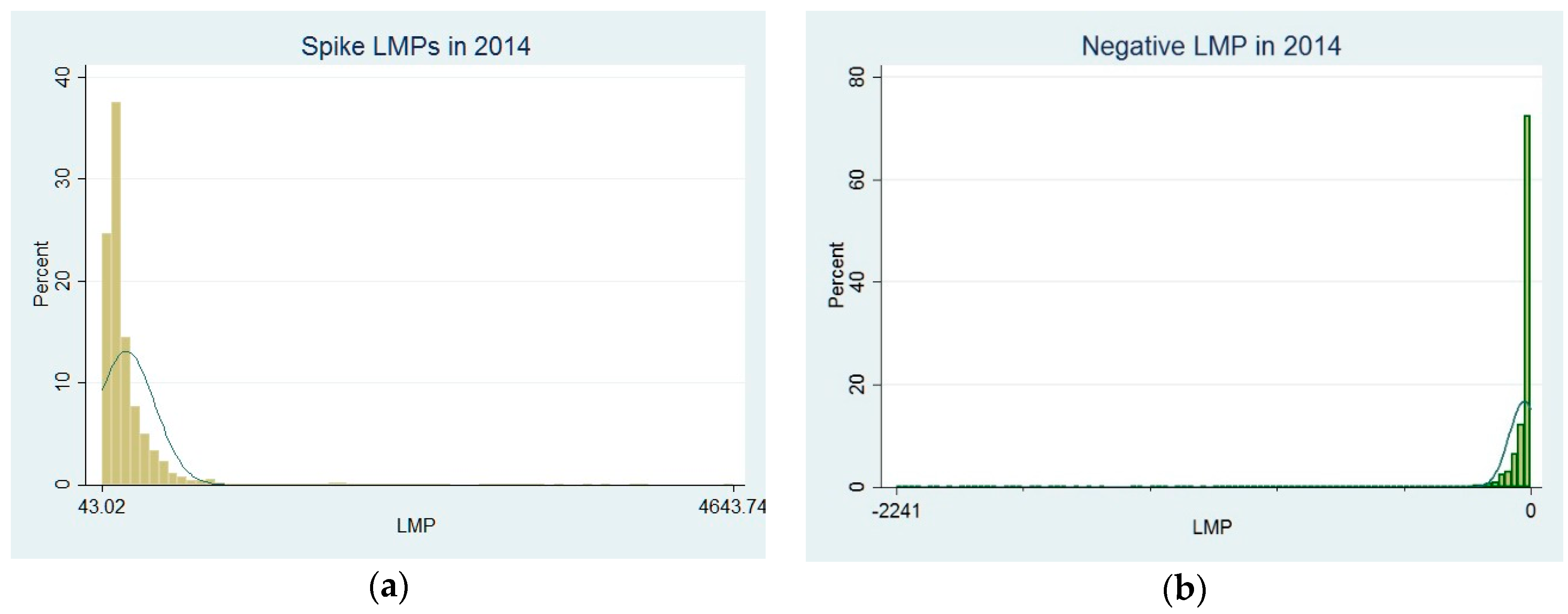
The description of our selected spike LMP
s is consistent with the peak load pricing defined by PJM. As shown in
Figure 1, almost 40% of annual spike LMP
s are clustered round
$120 in 2014. In order to improve the energy efficiency, PJM has a DR program that provides subsidies to customers who reduce load in response to price signals during the peak load time. This DR program includes an economic program, which sets up the trigger point at
$75 to make a subsidy payment, and an emergency program starting at
$500. The main body of our selected spike LMP
s, from the 5th percentile to the 95th percentile, is between
$87 and
$523, which is in line with the peak load prices in PJM’s DR program. Walawalkar et al. [
43] show that the optimal trigger point to assess spike LMP
s should start at
$66. Therefore, our selected spike LMP
s match those criteria by PJM’s DR Program and reflect the peak load scenarios.
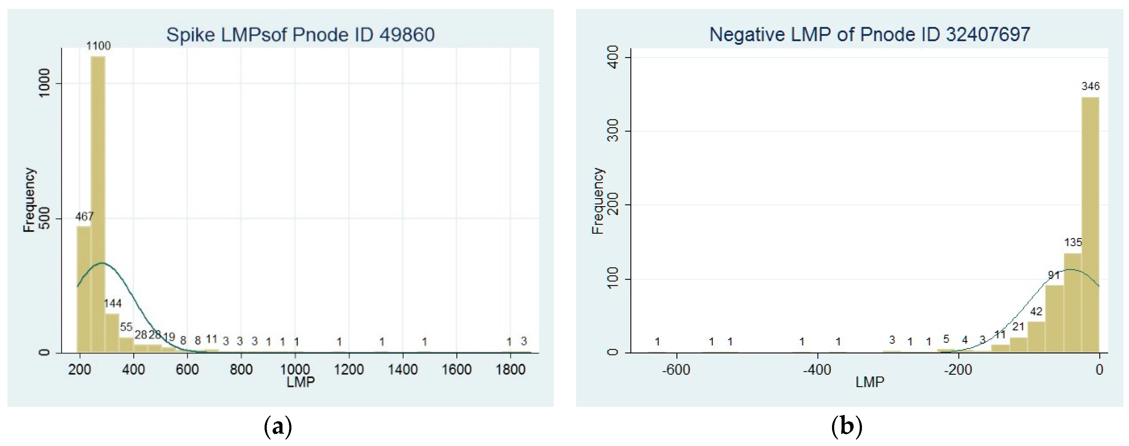
The occurrence of negative LMP
s is also significant across Pnode
s. Among the 11,574 Pnode
s, 11,444 of them have records of negative LMP
s. As depicted in
Figure 2, in Pnode ID.32407697, there are 668 records of negative LMP
s and these LMP
s count for 8% of the overall LMP
s in 2014. The smallest LMP is −
$630, and the majority of negative LMPs are located between −
$200 and 0. By contrast, the occurrences of spike LMP
s are even more prevalent. For example, in Pnode ID.49860, the qualified spike LMP
s show 1887 records and count for 22% of the overall LMP
s in 2014. Spike LMP
s range between
$190 and
$1875, and the majority of them are between
$200 and
$400. The prevalent occurrences of negative and spike LMP
s exacerbate the price swings across different Pnode
s.
We sort both categories of negative and spike LMPs by their Pnode IDs. For each Pnode and LMP category, we calculate the descriptive statistics, including mean, standard deviation, skewness, kurtosis, minimum, and maximum. We also calculate the percentage of occurrence for each group across Pnodes. For Pnode i, the percentage of negative LMPs is defined as
The percentage of spike LMPs is defined as
The descriptive results above have shown the severe and prevalent occurrence of both spike LMP
s and negative LMP
s. For further analyses, we use the 13 covariates listed in
Table 2. These covariates are categorized into two groups of spike LMP
s and negative LMP
s, and capture the position and dispersion of the two groups. We exclude the maximum of negative LMP
s because it is zero in all Pnode
s. We use these covariates to measure the cross-sectional variation for our PCA model in the next section.
4. Results and Discussion
4.1. PCA Results
Table 3 shows the correlation matrix for the covariates calculated from
Section 3. We observe many correlation values greater than 50%. Given this, it is necessary to apply a PCA model to effect a dimension reduction. By definition in
Section 2, PC
s are constructed as linear combinations of covariates with orthonormal loading coefficients. The first component, labeled PC1, is chosen to explain the largest proportion of variation in the covariates. The second component PC2 explains the second largest proportion of the variation that is left unexplained from the first component. PC3 continues explaining the remaining, and so forth.
Table 4 presents the variation explained by the eigenvalues of PCA. PC1, the component that has the largest eigenvalue 4.00, contributes 31% explanatory power of the variation of data. PC2 has the second largest eigenvalue (2.47) and explains 19% of the variation. The cumulative explanatory contribution by PC1 and PC2 reaches 50%, as shown in the cumulative column. Including the first six components, the cumulative explanatory contribution by PC1–PC6 already reaches 92%. Therefore, PCA helps reduce the dimensionality.
We extract the first six components. They are constructed as linear combinations of covariates so that they have orthonormal loading coefficients.
Table 5 presents how these PCs relate to our covariates and also presents the coefficients of covariates for each PC in the columns. For example, PC1 is expressed as the linear combination of our original covariates by the following equation:
As discussed in
Section 2, one advantage of PCA is that it helps discover the latent and structural meaning constructed by covariates. We can summarize the implication of each PC, which is generally qualitative and unobserved from direct regression by covariates. In Equation (10), among the covariates, three of them have significantly larger coefficients; namely,
Peak_Mean (0.4723),
Peak_Min (0.4457), and
Peak_Std (0.3565). These three covariates hold the dominant power to constitute PC1. They represent the position and dispersion of spike LMP
s. The mean (
Peak_Mean) and the minimum (
Peak_Min) control the position of spike LMP
s, while the standard deviation (
Peak_Std) quantifies the extent of dispersion.
We have found that as the foremost component, PC1 contributes 31% explanatory power of the variation of data. As the dominant composition for PC1, all the three covariates above belong to the spike LMP party. Therefore, we can infer that the variation of spike LMPs accounts for the overall population’s variation with larger power than that of negative LMPs.
Similarly, PC2 can be expressed as the linear combination of our original covariates by the following:
In PC2, we find that two covariates have significantly larger absolute values of coefficients: Neg_Std (0.4092) and Neg_Min (−0.4901). Both covariates are different from the dominant covariates for PC1, and they both are from the negative LMP party. Similar to PC1, PC2 can be interpreted as the position and dispersion of negative LMPs. PC2’s explanatory power is only 19%, implying that negative LMPs have less impact on the overall population’s variation.
For PC3, three covariates are dominant, as observed in
Table 5:
Peak_Max (0.4639),
Peak_Sku (0.4504), and
Peak_Kur (0.3969). They are duplicate as dominant covariates in PC1 or PC2, and all three are again from the spike LMP party. PC3 can be interpreted as the extent of concentration of spike LMP
s. Similarly, PC4’s dominant covariates are also the skewness and kurtosis of negative LMP
s (
Neg_Sku and
Neg_Kur), which makes PC4 the extent of concentration of negative LMPs. Compared with PC2, the explanatory powers of PC3 and PC4 become even weaker (16% and 13%). PC3’s value is greater than PC4’s, implying again that spike LMP
s still account for more variation than negative LMP
s.
There is only one covariate that dominates in each of PC5 and PC6. In PC5, the only covariate is
Neg_Mean (0.9815), and in PC6, the only one is
Neg_Per (0.7223). As shown in
Table 4, PC5 and PC6 have only 8% and 5% explanatory power, respectively. They are supplementary variation affected by negative LMP
s.
We have finished the analyses of PC1–PC6. According to their dominant covariates, we further elaborate the implication of each PC by renaming them as follows:
PC1: the position and dispersion of spike LMPs;
PC2: the position and dispersion of negative LMPs;
PC3: the concentration of spike LMPs;
PC4: the concentration of negative LMPs;
PC5: the average of negative LMPs;
PC6: the probability of occurrence of negative LMPs.
In summary, through the result of PCA, we select six components and interpret their implication related to the covariates. We find that components highly related to spike LMPs account for the variation of electric prices with larger power than those related to negative LMPs. In the next part, we further examine our statement using PCR.
4.2. PCR
After constructing PC
s, we apply them as the independent variables in the PCR. As these PC
s are orthonormal between each other, the PCR model can avoid multi-collinearity as a replacement of traditional multiple regressions. In order to investigate how negative and spike LMP
s affect the cross-Pnode price volatility, we present the following PCR model:
is the overall standard deviation of LMPs in Pnode
i. In order to compare the importance across PC
s, we use the standardized
β coefficients. The PCR results are presented in
Table 6. For the price volatility of a Pnode, PC1 is the largest factor with a 0.91
β coefficient. This suggests that the occurrence of spike LMP
s is the foremost condition to cause high volatility. By contrast, PC2 has only 0.36 as the second largest
β, suggesting that the performance of negative pricing is far less important to trigger large price fluctuations. None of the remaining PC
s related to negative LMP
s have a comparable impact to PC1. Moreover, among these negative-LMP
s-related PC
s, PC4 is even not statistically significant in the PCR. This further shows that reducing the occurrence of spike LMP
s is the essential resolution to control the high price volatility.
In summary, our results from PCA and PCR suggest that the performance and distribution of spike prices account for more price volatility in the electricity RTOs with numerous transmission lines. We are aware that negative prices indicate over-supply, while spike prices indicate over-demand. Therefore, in order to improve the price forecast, issues about demand inflexibilities should be taken into account to a greater extent. By comparison, the appearance of negative prices does not dominate in terms of both amount and impact on the overall price swings.
4.3. Discussion
Modern smart grid systems have multiple responsibilities and missions beyond a primitive-stage transmission center. Take PJM as an example. Besides the maintenance of software, networks, and hardware units, today’s PJM plays a more important role in the changes including (1) the establishment and enforcement of the trading rules, regulations, and protocols for market participants; (2) the decision-making of market-clearing settlement prices; and (3) the oversight of legitimate market competition [
42]. These new changes are attributed to the new responsibility of the modern smart grid systems, that is, to provide a stable market environment for the production, transmission, and trading of electricity. The new responsibility makes the smart grid electric system more and more market-alike, as stated by the authors of [
44]. The tendency of marketization in the smart grid electric systems even has influence over the long-term sustainable development plans of power generation and transmission facilities [
42]. Therefore, the economic perspective of this study conforms to the sustainable development of the modern smart grid system, and the outcomes of this study contribute to the responsibility of the modern smart grid systems for a stable electricity market environment.
The massive negative LMP
s and spike LMP
s are both the signal of inequilibrium of power supply and demand. As a signal of excessive supply, the occurrence of negative LMP
s is a possible outcome of renewable energy sources. Some types of renewable energy are largely promoted by the adoption of incentive mechanisms [
19,
20]. For example, the U.S. government gives
$26/MWh as a wind production tax credit, which makes wind generators continue producing but still profit at a negative price. However, as reflected by negative LMP
s, these over-supply cases fail to offset the large demand cases, which explains the coexistence of massive negative LMP
s and spike LMP
s in the market. The mismatch between excessive supply and excessive demand is caused by both timing and locational issues. Let us still use wind energy as the example. Lack of transmission capacity means the wind energy cannot be transmitted outside the region where the power is generated to places with excessive demand in the meantime [
16]. The seasonality of wind makes the wind energy source fail to become a steady supplier to meet the uncertain excessive demand.
According to the principle of economics, to solve the large price fluctuations, the key is to coordinate the power supply and demand. As stated in the works of [
41,
42], the biggest difference between the electricity market and other commodity markets is the non-storable property of the electricity. In economics, the capacity of storage enables the products and services to transfer from time to time, and transfer the surplus to fulfill shortage, so as to achieve the market efficiency and equilibrium. Therefore, if the electric power can be easily stored and transferred across time periods, it will be indifferent from the other regular products and services.
Thus, during the recent years, EES has been considered as one potentially effective and technical resolution to the power inequilibrium. The development of EES helps reduce and remove the inequilibrium cases for both types. RTO can use EES devices to adjust the over-supply and peak-demand time and thus reduce the time-series imbalance as stated by recent studies. For example, Li et al. [
45] find that specific calendar anomalies exist in the electricity market and induce the time-series imbalance. Liu et al. [
46] state that EES can improve economic efficiency in a wholesale electricity market by saving the electricity during the low-LMP hours for the high-LMP hours. Sioshansi et al. [
21] point out that EES can achieve the practice of arbitrage—the ability to buy at low prices and discharge at high prices, which facilitates the adjustment of market prices. Our empirical findings have shown that there are a number of large price fluctuations as the reflection of power inequilibrium. Our finding is in line with the previous studies about EES [
14,
16,
21,
45]. Therefore, the application of EES can be a potential and technical resolution.
Additionally, as another possible resolution, improving the transmission capacity may also help reduce the power inequilibrium. Because of the high cost of transmission loss and the congestion, the loss of power in the transmission has been an issue about the power imbalance across regions. As one important mission of the smart grid system development, improving the transmission capacity may encourage the power flow from over-supply regions to over-demand regions, and help solve the spatial power inequilibrium. Furthermore, as mentioned before, PJM has initiated a DR program and provides subsidies to customers who reduce load in response to price signals during the peak load time. According to the authors of [
21,
43], the DR program is an economic program, and gives incentives for reduction of the price fluctuations.
In order to implement these resolutions, the premise is to have a comprehensive and concrete understanding on the current status of energy demand and supply in the whole energy system. In this study, we employ an effective method of PCA and PCR to distinguish and explore the inequilibrium of energy demand and supply from the perspective of economics. We take the energy price as the key signal to examine the inequilibrium of energy demand and supply in the smart grid energy system. The economics-related analyses can help identify the current status of energy demand and supply, figure out the main driver of the power inequilibrium, distinguish the flaws of the smart grid energy system, and consequently improve the energy efficiency and load management.
5. Conclusions
The modern electricity system is pursuing energy efficiency and optimized load management. In this study, we observe the efficiency of energy transition from the standpoint of economics, by employing a big-data study in the wholesale electricity market with advanced smart grid configurations. We focus on spike and negative prices, two frequently-observed phenomena and the constituents of extreme values with opposite economic meanings. Negative prices indicate over-supply, while spike prices indicate over-demand. This study assesses the impact of negative pricing and spike pricing on price fluctuation. We evaluate price fluctuation by the standard deviation of RTPs for each transmission line. We analyze the RTP data from the PJM electricity market including 11,574 transmission lines with hourly updated records. For both negative and spike price groups, we calculate 13 covariates by transmission lines. These covariates capture the distributions of spike prices and negative prices, respectively.
To compare the effects on price fluctuations between negative prices and spike prices, we employ a PCA model. We find that, firstly, the PC that represents the position and dispersion of spike prices has the largest explanatory power of the overall variation. By contrast, PCs dominated by negative pricing have much smaller explanatory power. Next, we run a PCR model and examine how these PCs affect the price fluctuation. Our results indicate that the performance and distribution of spike prices account for price fluctuations with larger explanatory power than those of negative prices, and the results apply to all the incorporated transmission lines.
In practice, our results indicate that in the current electricity market, although types of renewable energy generators have already been participating and making a contribution, the over-demand and energy shortage are still the big issues. The time-varying inequilibrium between power supply and demand are common in any area. From the perspective of policy makers, developing EES and DR and upgrading the transmission capacity should be the resolution to reducing market price fluctuations.
In theory, our results suggest that PCA and PCR are efficient tools for electricity market analyses. Using PCA, we can reduce the dimensionality of multivariate analysis, and discover the structural meaning of factors by constructing latent common structures. In this study, we figure out many findings that are unobservable when we use the original covariates. The latent structures can also be applied into the PCR for further analysis. Therefore, our study confirms the advantage of PCA and PCR as efficient tools for electricity market studies.


