Well-to-Wheels Approach for the Environmental Impact Assessment of Road Freight Services

Abstract

The diffuse nature of road transport and the heterogeneity of heavy vehicles have hindered the implementation of emissions accounting systems. Even though there are emission factors in well-known databases, these factors have commonly been designed in industrialized countries, which might have geography, type of roads, and operating conditions different to other countries. This paper proposes a method for the energy consumption and emissions estimation based on vehicle operating conditions in regions with different topology, such as Colombia, Malaysia, and Spain, as case studies. Moreover, the environmental impacts of fuel production in each country are calculated. The diesel consumption on mountainous roads for a full loaded rigid truck in Colombia was 45 L/100 km, compared to averages between 22–26 L/100 km from other sources usually applied. In contrast, the diesel consumption for an articulated truck on a hilly road in Spain from both the proposed method and generic databases coincided in 31 L/100 km. The vehicle speed, load, and road gradient also generated large variations up to 145% in the air pollutants’ estimation. This study contributes to the need for more research about emission factors and tools that facilitate and reduce uncertainty in the environmental accounting in freight companies in different geographies.

1. Introduction

Despite the fact that sustainable development has been considered a topic of interest since the 1980s [1,2], the transport sector has been one of the last sectors to develop relevant initiatives aimed at optimizing its operations from the environmental perspective. The road freight sector has been more concerned with minimizing the time and costs of its activity with the application of vehicle routing models since the 1950s [3], or developing their own mathematical algorithms for the optimization of their activity based on the specific variables on the types of products, clients, type of fleet, geographical situation, etc. [4]. These improvements have led, without it being its main objective, to fuel savings per ton-kilometer (tkm) transported and reductions of their environmental impacts. However, taking Europe as an example, while all sectors reduced a quarter of their greenhouse gas (GHG) emissions between 1990 and 2009, the transport sector increased almost a third of its emissions in the same period [5]. This was mainly due to the increase in the domestic truck traffic, which despite representing only 3% of the vehicle fleet in the European Union (EU), produces almost a quarter of the total CO₂ emissions generated by the road transport sector [6]. The CO₂ emissions produced by road freight increased by 36% between 1990 and 2010 [7]. This increase stopped in 2010 due to the European economic crisis that began between 2008 and 2009. However, some projections have suggested that under this perspective, without the intervention of governments, GHG emissions produced by trucks will be, with respect to the 1990 levels, around 35% higher for the years, 2030 and 2050 [8].

The energy consumption and GHG emissions of the sector are not being reduced as expected, mainly due to the difficulties in implementing energy efficiency measures in the road freight subsector and the difficulty of finding alternatives to diesel fuel [9]. In contrast to the industrial sector where real-time emissions can be easily measured and thus different emission regulation and trading mechanisms can be established [10], in the transport sector, due to its diffuse nature, the establishment of these mechanisms has been hampered. Policy planning for traffic emissions has commonly consisted of sub-national or municipal strategies, such as the implementation of low-emission zones or the improvement of traffic flow to reduce the concentration of air pollutants in specific areas, but these types of measures, instead of reducing them, are dispersing these air pollutants over a bigger geographical area [11]. Measures to effectively reduce the environmental impacts in this sector have consisted in limiting, through regulations, the emissions of air pollutants, such as carbon monoxide (CO), nitrogen oxides (NOx), volatile organic compounds (VOC), and particulate matter (PM), of newly manufactured vehicles prior to entering the market [12]. The existing regulations for the control of air polluting emissions around the world are based almost generally on the European standards [13], US Environmental Protection Agency (EPA) [14], or Japanese regulations [15], from which most countries directly take the established limits for the specific standard or reference the limitation values of different standards [16,17]. Truck manufacturers have concentrated efforts into meeting these demanding standards by modifying engines and installing devices for the post-treatment of exhaust gases, such as exhaust gas recirculation valves and particulate filters, in order to reduce NOx and PM emissions, respectively. However, these efforts have negatively affected the fuel efficiency [18,19,20]. In recent years, some manufacturers have shown technological improvements to meet the Euro VI standards by using selective catalytic reduction systems that use urea to reduce NOx emissions without significantly affecting the fuel consumption, obtaining a diesel consumption of up to 28 L/100 km for articulated trucks under optimal road and driving conditions during efficiency tests [21,22].

Although countries, such as Japan, the United States, Canada, and China [8,23], have incorporated legislative measures for the control of CO₂ emissions, the EU has yet to establish limits for these emissions from road freight heavy vehicles. In the EU, among the first initiatives to tackle GHG emissions was the Communication 2014/285 [8] “Strategy to reduce fuel consumption and CO₂ emissions in heavy vehicles”. In addition, the series of documents that accompanied this communication highlighted the absence of GHG control measures as well as common and internationally recognized standards for their measurement. Recently, a surveillance system for heavy vehicles in the EU was proposed through a regulation that is expected to be published in 2019, which requires manufacturers to provide accurate data on the CO₂ emissions of their new trucks in order to collect information that will allow the future establishment of limits to GHG truck emissions in a suitable and uniform way [23]. Despite the absence of measures to control CO₂ emissions during vehicle operation, the transport sector, particularly, freight transport, has voluntarily adopted standards to account for these emissions and energy consumption. Freight companies have been prompted by other sectors that have demanded a reduction in their contribution to the carbon footprint of their products, goods, or services. In Europe, the carbon footprint calculation has become popular since the entry into force of Directive 2003/87/EC [24], which requires mandatory GHG reporting by companies in the energy and industrial subsectors with the highest energy use. Companies in other diffuse sectors, who were not included until 2009 in the Emissions Trading Scheme [25], began to take an interest in their carbon footprint due to the benefits that it could bring to their organization and their products, such as higher market value, an increase in brand value, corporate image improvement, reduced insurance fees as well as an improvement in their credit ratings [26]. Among these initiatives for fuel consumption and emissions accounting, they can be referenced to the related general tools for life cycle analysis, such as SimaPro [27], GaBi [28], Gemis [29]; specific tools for the transport sector include Tremove [30], COPERT [31], MOVES [32], GREET [33], the decarbonization prediction model [34], EcoTransIT [35], the GHG Protocol tool for mobile combustion [36], the World Ports Climate Initiative (WPCI) Carbon Footprinting Calculator [37], the Third Party Road Freight CO₂ emissions pilot model [38], the Network for Transport Measures (NTM) basic Freight Calculator [39], Planung Transport Verkehr (PTV) Map & Guide [40], Logistics Emissions Calculator (LogEC) [41], Versit+ [42]; and databases, reports, or methodologies, such as the European standard (EN) 16258 [43], the GHG Protocol Corporate Standard [44], the European Association for Forwarding, Transport, Logistics and Customs Services (CLECAT) guide [45], Odette [46], Panteia and Duoinlog [47], the Intergovernmental Panel on Climate Change (IPCC) [48], Ecoinvent [49], IDEMAT [50], the Handbook of Emission Factors for Road Transport (HBEFA) [51], Lipasto [52], the GHG Reporting Database [53], the Department for Environment, Food and Rural Affairs (DEFRA) GHG conversion factors [54], the European Monitoring and Evaluation Programme and the Environmental European Agency (EMEP/EEA) emission inventory guidebook [55], the Joint Research Centre (JRC) technical reports [56], and the Netherlands Organisation for applied scientific research (TNO) reports [57].

Most of the aforementioned tools are currently based on the standard EN-16258 [43] “Methodology for the calculation and declaration of energy consumption and greenhouse gases emissions in transport services (transport of goods and passengers)”. This standard is the first international standard to harmonize and standardize the procedures for the calculation and reporting of emissions and energy for the transport sector. This standard has been fully accepted among the European transport companies [58] and represents a possible basis for future international standardization initiatives [59]. The EN-16258 [43] focuses the reporting of energy consumption and GHG emissions on the fuel life cycle analysis (Well-to-Wheels, WTW). The WTW analysis includes the generated impacts by the energy use in the vehicle (Tank-to-Wheels, TTW), plus the impacts of the extraction of the raw materials, transportation, transformation, and distribution of the fuel to the service station (Well-to-Tank, WTT). However, limiting the emissions accounting just to the GHGs narrows the analysis only to the climate change impact, leaving aside other environmental impacts associated with road freight services. Although accounting the energy consumption during the vehicle operation can calculate the fuel-dependent pollutants other than CO₂, such as emissions of sulfur dioxide (SO₂) and heavy metals contained in the fuel, the emissions of CO, NOx, methane (CH₄), nitrous oxide (N₂O), ammonia (NH₃), PM, and non-methane volatile organic compounds (NMVOC) do not depend proportionally on fuel consumption, but on other factors, such as the emission control technology and operating conditions. The emissions estimation through the mentioned tools for road transport commonly base the results on factors that only consider operation parameters, such as vehicle size, emission control technology, and some also look at the load factor, except for tools [31,32] that consider other important factors, such as the vehicle speed and the road gradients. However, the main limitation using even the most comprehensive available tools is the impossibility of considering the variations in speed and road gradients in the different slopes during a specific freight service. Therefore, it is necessary to use emission factors and a methodology that provides accurate results for each assessed case. Until there is a procedure for measuring pollutant emissions for diffuse sectors, its estimation is the only way to establish the objectives for its reduction and measure its degree of achievement. The emission factors and the fuel consumption calculation models that are incorporated in the different tools must be susceptible to improvements and updates based on experimentally obtained information.

This work aimed to advance research along that line. On the one hand, a method was proposed for the calculation of fuel consumption and TTW emissions during a road freight service. The method was based on the proposed procedure in the EMEP/EEA air pollutant emission inventory guidebook of 2016 [55] and incorporated variables related to the characteristics of the route and the service itself that were identified from the study of three experiments. These adjustments allowed us to estimate more accurately fuel consumption to the actual measured figures, and consequently reduce the error of the proportional emissions. On the other hand, the emission factors were adjusted based on the inventory analysis for fuels other than 100% diesel fossil fuel, which affects the reliability of the estimation of the WTW emissions [60]. From the results of the emission inventories for the WTT and TTW phases obtained with the new calculation method, an environmental impact assessment was performed for the three cases under study through the ReCiPe 2016 [61] method with the tool for life cycle analysis SimaPro 8.5.0 [27] and the Ecoinvent v3.4 [49] database. Given that the production of fuels can generate impacts in categories other than those mainly affected by emissions from the operation of the vehicles, such as climate change, acidification, eutrophication, ozone depletion, and energy consumption [62,63], the 18 impact categories of the assessment method were considered.

2. Materials and Methods

In 2017, the EEA published the “EMEP/EEA air pollutant emission inventory guidebook 2016” [55], which details the calculation methods and factors for fuel consumption and emissions with three levels of precision (tiers) for the vehicle operation phase or TTW analysis. These emission factors compiled in the EMEP/EEA [55] guide were based on previous initiatives, such as Artemis [64], Corinair [65], the Methodologies to Estimate Emissions from Transport (MEET) project [66], and HBEFA emission factors [51].

The calculation model proposed by EMEP/EEA [55] offers three approaches with different consumption and emission factors, depending on the data availability. Tier 1 provides emission factors based on the amount (kg) of fuel; Tier 2 provides emissions and fuel consumption factors per km traveled for different vehicle types and emission control technologies; and Tier 3 establishes a series of equations and factors to incorporate, in addition to the variables included in the Tier 2 method, others, such as the speed, the load factor, and the road gradient.

It should be noted that the Tier 2 and Tier 3 emission factors available for freight vehicles are only for diesel and gasoline engines, considering the correction factors for biodiesel and bioethanol mixtures, respectively. The considered emissions by the EMEP/EEA [55] guide can be classified into four groups:

• Group 1: Pollutants not directly dependent on fuel consumption, such as CO, NOx, CH₄, N₂O, NH₃, NMVOC, and PM_2.5.
• Group 2: Estimated emissions based on the fuel, lube oil, and urea consumption, such as CO₂, SO₂, and heavy metals.
• Group 3: Emissions of polycyclic aromatic hydrocarbons (PAHs), persistent organic pollutants (POPs), and dioxins and furans.
• Group 4: NMVOC emissions, such as alkanes, cycloalkanes, alkenes, alkynes, aldehydes, and aromatics, calculated as a fraction of the total NMVOC.

In addition to these pollutants derived from fuel, lube oil, and urea consumption, emissions from tires, brakes, and road surface abrasion were considered.

The proposed method for the energy consumption and emissions estimation for a specific road freight service basically seeks to individually analyze different sections of the route considering changes in the operating parameters, such as average speed and road gradient, as determined through the Google Earth Pro software [67]. The accounting of emissions was elaborated based on the Tier 3 factors, equations, and coefficients from the EMEP/EEA [55] guide.

The calculation of each of these pollutants was performed for each section of the route, which was divided considering significant changes in the circulation area (urban or interurban), number of lanes, traffic density, average speed, topology, or trend in the road gradient. The energy consumption, emission factors, and calculation equations for each group of pollutants are detailed in the following subsections.

2.1. Pollutants of Group 1

For the estimation of CO, NOx, VOC, and PM_2.5 emissions and energy consumption, the Tier 3 method was used. For the CH₄, N₂O, and NH₃ emissions, the Tier 2 emission factors were used, which are available by vehicle type, control emissions technology, and type of road circulation.

The Tier 3 method provides the coefficients for each type of vehicle and the emission control technology (conventional, Euro I–VI), load factor (0%, 50%, and 100%), and the road gradient (0%, ±2%, ±4%, and ±6%), based on the speed in each route section to be applied in Equation (1) [55]:

$$ECorEF=\frac{\alpha \times V^2+\beta \times V+\gamma +\frac{\delta }{V}}{\epsilon \times V^2+\mathsf{\zeta }\times V+\mathsf{\eta }}\times \left(1-RF\right)$$

(1)

where EC is the Energy Consumption (MJ/km); EF is the emission factor of CO, PM_2.5, NOx, and VOC (g/km); V is the vehicle speed (km/h); and RF a reduction factor. Coefficients (α, β, γ, δ, ε, ζ, η) and the RF are obtained from the 1.A.3.b.i-iv Road transport hot EFs Annex 2017, attached in the EMEP/EEA report [55].

Based on the obtained results using the EMEP/EEA Equation (1) and the coefficients for 0% and 100% load factors, it is possible to calculate the energy consumption or emission factor for a partial load using the Equation (2), where the specific load factor, LF, is from 0 to 1.

$${(ECorEF)}_{LF}={((ECorEF)}_{empty}+(ECorEF{)}_{full}-{(ECorEF)}_{empty})\times LF$$

(2)

For the estimation of CH₄, N₂O, NO₂, and NH₃ gases, the emission factors per km were directly applied from

Table A1. CH₄ emission factors for heavy vehicles (mg/km) (Own elaboration based on data from EMEP/EEA [55]).

Type of Vehicle	Type of Road
	Urban	Rural	Motorway
Gross vehicle weight < 16 t	85	23	20
Gross vehicle weight > 16 t	175	80	70

,

Table A2. Reduction rates for CH₄ emissions for diesel heavy vehicles (%) (Own elaboration based on data from EMEP/EEA [55]).

Euro Standard	Type of Road
	Urban	Rural	Motorway
Euro II	36	13	7
Euro III	44	7	9
Euro IV	97	93	94
Euro V and earlier	97	93	94

,

Table A3. N₂O emission factors for diesel heavy vehicles by type of road (mg/km) (Own elaboration based on data from EMEP/EEA [55]).

Euro Standard	Rigid Truck 7.5–12 t			Rigid and Articulated 12–28 t			Rigid and Articulated 28–34 t			Articulated > 34 t
	Urban	Rural	Motorway	Urban	Rural	Motorway	Urban	Rural	Motorway	Urban	Rural	Motorway
Pre-Euro	30	30	30	30	30	30	30	30	30	30	30	30
Euro I	6	5	3	11	9	7	17	14	10	18	15	11
Euro II	5	5	3	11	9	6	17	14	10	18	15	10
Euro III	3	3	2	5	5	4	8	8	6	9	9	7
Euro IV	6	7.2	5.8	11.2	13.8	11.4	17.4	24.4	17.4	19	23.4	19.2
Euro V	15	19.8	17.2	29.8	40.2	33.6	45.6	61.6	51.6	49	66.6	55.8
Euro VI	18.5	19	15	37	39	29	56.5	59.5	44.5	61	64	48

and

Table A4. Fraction of NO₂ in NOx emissions and NH₃ emission factors for diesel heavy vehicles. (Own elaboration based on data from EMEP/EEA [55]).

Euro Standard	NO2 in NOx	NH3
	%	(mg/km)
Pre-Euro	11	3
Euro I–Euro II	11
Euro III	14
Euro IV	10
Euro V	12	11
Euro VI	8	9
Euro III + CRT *	35

* Continuously Regenerating Trap

. For the effect of biodiesel blends on emissions, the average emissions of CO, PM_2.5, NOx, and VOC were determined by the application of the variation rates presented in

Table A5. Variation rate of emissions for diesel heavy vehicles with biodiesel blends (Own elaboration based on data from EMEP/EEA [55]).

Pollutant	Biodiesel Blend
	B10	B20	B100
CO	−5%	−9%	−20%
PM	−10%	−15%	−47%
NOx	3%	3.5%	9%
VOC	−10%	−15%	−17%

, which are only recommended for Euro III or earlier vehicles, since for more modern vehicles, the variation is more difficult to predict due to the implementation of exhaust gas treatment systems [55].

2.2. Pollutants of Group 2

2.2.1. Pollutants from fuel consumption

For the estimation of CO₂ and SO₂ emissions, the fuel characteristics were considered, such as the content of sulfur (s), carbon (c), hydrogen (h), oxygen (o), and nitrogen (n). From these characteristics in mass terms, for the CO₂ calculation, Equations (3)–(5) were applied [55]:

$$r_{H:C}=11.916\frac{h}{c}$$

(3)

$$r_{O:C}=0.7507\frac{o}{c}$$

(4)

$$E_{C{O}_2}=44011\times \frac{E{C}_m}{12011+1008r_{H:C}+16000r_{O:C}}$$

(5)

where $E_{C{O}_2}$ are the CO₂ emissions (kg) and $E{C}_m$ is the energy consumption (kg). If biofuel blends are used, the calculation of CO₂ emissions should be made by only considering the fraction of fossil diesel.

For the SO₂ calculation, Equations (6) and (7) were applied [55]:

$$S_m=s\times {10}^{-6}.$$

(6)

where s is the sulfur content in parts per million (ppm).

$$E_{S{O}_2}=2\times S_m\times E{C}_m$$

(7)

where $E_{S{O}_2}$ are the SO₂ emissions (g), and $S_m$ is the sulfur content (g/g).

The emission factors of heavy metals in ppm contained in the consumed fuel by heavy vehicles are presented in

Table A6. Emission factors of heavy metals in fuel and lube oil in diesel heavy vehicles in (Own elaboration based on data from EMEP/EEA [55]).

Source	Lead	Cadmium	Copper	Chromium	Nickel	Selenium	Zinc	Mercury	Arsenic
Fuel	0.0005	0.00005	0.0057	0.0085	0.0002	0.0001	0.018	0.0053	0.0001
Oil	0.0332	4.56	778	19.2	31.89	4.54	450.2	0	0

.

2.2.2. Pollutants from lube oil consumption

The consumption of engine lube oil for heavy diesel trucks is on average 1.56 kg/10,000 km with an average CO₂ emissions of 0.486 g/km [55]. From this consumption, the content of heavy metals in the lube oil used by heavy vehicles are presented in Table A6.

2.2.3. Pollutants from urea consumption

In Euro V and Euro VI heavy-duty diesel engines, urea is used as a catalyst to reduce NOx emissions. The urea consumption generates CO₂ emissions, whose average emission factor is 0.26 kg CO₂/L or 0.238 kg CO₂/kg of urea solution [55]. The urea solution has an urea content of 32.5% [68]. If the amount of consumed urea is unknown, this consumption is assumed to be 6% or 3.5% of the diesel consumption in Euro V or Euro VI heavy vehicles, respectively [55].

2.3. Other Pollutants

For the estimation of pollutants included in Group 3, the emission factors for diesel heavy vehicles for PAHs and POPs are presented in

Table A7. Emission factors for PAHs and POPs (Own elaboration based on EMEP/EEA [55]).

Pollutant	μg/km	Pollutant	μg/km
Indeno(1,2,3-cd) pyrene	1.40	Benzo(j)fluoranthene	13.07
Benzo(k)fluoranthene	6.09	Benzo(a)anthracene	2.39
Benzo(b)fluoranthene	5.45	Fluorene	39.99
Benzo(ghi)perylene	0.77	Chrysene	16.24
Fluoranthene	21.39	Phenanthrene	23.00
Benzo(a)pyrene	0.90	Napthalene	56.00
Pyrene	31.59	Anthracene	8.65
Perylene	0.20	Coronene	0.15
Benzo(b)fluorene	10.58	Dibenzo(ah)anthracene	0.34
Benzo(e)pyrene	2.04	Perylene	0.20
Triphenylene	0.96	Benzo(b)fluorene	10.58

, and those for the polychlorinated dibenzo dioxins (PCDDs), polychlorinated dibenzo furans (PCDFs), and polychlorinated biphenyls (PCBs) are presented in

Table A8. Emission factors for PCDDs, PCDFs, and PCBs (Own elaboration based on data from EMEP/EEA [55]).

Euro Standard	Pollutant (pg/km)
	PCDD	PCDF	PCB
Pre-Euro	25	38	10.9
Euro I	25	38	12.6
Euro II	25	38	12.6
Euro III	25	38	12.6
Euro IV	25	38	12.6
Euro V	0.31	0.45	0.15
Euro VI	0.16	0.24	0.08

.

For the pollutants included in Group 4, the fractions of alkanes, cycloalkanes, alkenes, alkynes, aldehydes, and aromatics, corresponding to 96.71% of the total NMVOC, are presented in

Table A9. Pollutants included in Group 4; fraction of the total NMVOC (Own elaboration based on data from EMEP/EEA [55]).

Sub-group	Pollutant	% Weight	Sub-group	Pollutant	% Weight
Alkanes	Ethane	0.03	Aldehydes	Formaldehyde	8.4
	Propane	0.1		Acetaldehyde	4.57
	Butane	0.15		Acrolein	1.77
	Isobutane	0.14		Benzaldehyde	1.37
	Pentane	0.06		Crotonaldehyde	1.48
	Heptane	0.3		Metacrotine	0.86
	2-methylhexane	0.63		Butyraldehyde	0.88
	2-methylheptane	0.21		Isobutanaldehyde	0.59
	3-methylhexane	0.35		Propionaldehyde	1.25
	Dean	1.79		Hexanal	1.42
	3-methylheptane	0.27		I-valeraldehyde	0.09
	Alcanes c > 13	27.5		Valeraldehyde	0.4
				O-tolualdehyde	0.8
				M-tolualdehyde	0.59
			Aromatics	Toluene	0.01
				M.p-xylene	0.98
				O-xylene	0.4
Alkenes	Ethylene	7.01		1.2.3-trimethylbenzene	0.3
	Propylene	1.32		1.2.4-trimethylbenzene	0.86
	Isobutene	1.7		1.3.5-trimethylbenzene	0.45
	1,3-butadiene	3.3		Styrene	0.56
				Benzene	0.07
				Aromatic c9	1.17
				Aromatics c > 13	20.37
Cycloalkanes	All	1.16	Alkynes	Acetylene	1.05

. The residual amount, that is, 3.29% of the total NMVOC, were considered HAPs.

The abrasion of brakes, tires, and the road surface generates particulate matter (PM_>10, PM_2.5–10, and PM_<2.5) that contains metal and non-metal particles that are released into the air, water, and soil. The emission of particles from tire and brake abrasion was calculated based on the weight, number of axes, and speed in each section of the route; hence, this method was considered as Tier 2+.

For the calculation of the total particulate matter (TPM) of the tire abrasion of heavy vehicles, Equations (8) and (9) were applied [55]:

$$LC{F}_N=1.41+\left(1.38\times LF\right)$$

(8)

$$\mathrm{T}P{M}_N=\frac{N_{axes}}{2}\times LC{F}_N\times 0.0107\times SC{F}_N$$

(9)

where $LF{C}_N$ is the load correction factor for tire abrasion; $N_{axes}$ is the number of axes; $\mathrm{T}P{M}_N$ is the total PM emission of tire abrasion (g/km); and $SC{F}_N$ is the speed correction factor for tire abrasion. If V < 40 km/h, then $SC{F}_N=1.39$; if 40 km/h ≤ V ≤ 90 km/h, then $SC{F}_N=\left(-0.00974\times V\right)+1.78$; and if V > 90 km/h, then $SC{F}_N=0.902$.

For the calculation of the TPM of brake abrasion in heavy vehicles, Equations (10) and (11) were applied [55]:

$$LC{F}_F=1+\left(0.79\times LF\right)$$

(10)

$$\mathrm{T}P{M}_F=3.13\times LC{F}_F\times 0.0075\times SC{F}_F$$

(11)

where $LC{F}_F$ is the load correction factor for brake abrasion; $\mathrm{T}P{M}_F$ is the total PM emissions of brake abrasion (g/km); and $SC{F}_F$ is the speed (V) correction factor for brake abrasion. If V < 40 km/h, then $SC{F}_F=1.67$; if 40 km/h ≤ V ≤ 95 km/h, then $SC{F}_F=\left(-0.0270\times V\right)+2.75$; and if V > 95 km/h, then $SC{F}_F=0.185$.

For the calculation of the TPM from road surface abrasion by heavy vehicles, an average factor of 0.076 g/km was used [55]. From the TPM emissions calculated for each origin, it is necessary to specify what type of particles are contained in this total by the fractions shown in

Table A10. Fraction of PM_>10, PM_2.5–10, and PM_<2.5 content in the TPM by source (Own elaboration based on data from EMEP/EEA [55]).

	Tires	Brakes	Road Surface
PM>10	40%	2%	50%
PM2.5–10	18%	59%	23%
PM<2.5	42%	39%	27%
TPM	100%	100%	100%

. Additionally, in the TPM emissions of tires and brakes, there is a content of different metal and non-metal elements and PAHs, which are presented in

Table A11. Content of PAHs and chemical elements in ppm of the TPM from tire and brake abrasion (Own elaboration based on data from EMEP/EEA [55]).

Element	Tires	Brakes	Element	Tires	Brakes
Benzo(a)pyrene	3.9	0.74	Magnesium cation (Mg2+)	166	44,570
Benzo(b)fluoranthene	0	0.42	Manganese (Mn)	51	2460
Benzo(k)fluoranthene	0	0.62	Molybdenum (Mo)	2.8	10,000
			Sodium (Na+)	645	7740
Silver (Ag)	0.1	0	Ammonium cation (NH4+)	190	30
Aluminum (Al)	324	2050	Nickel (Ni)	29.9	327
Arsenic (As)	3.8	67.5	Nitrate (NO3−)	1500	1600
Barium (Ba)	125	38,520	Lead (Pb)	176	6072
Bromine (Br)	20	40	Rubidium (Rb)	0	50
Calcium (Ca)	892	770	Sulfur (S)	1100	12,800
Cadmium (Cd)	4.7	22.4	Antimony (Sb)	2	10,000
Chlorine (Cl)	520	1500	Selenium (Se)	20	20
Chloride (Cl-)	600	1500	Silicon (Si)	1800	67,900
Cobalt (Co)	12.8	6.4	Sulfate (SO4−)	2500	33,400
Chromium (Cr)	23.8	2311	Tin (Sn)	0	7000
Copper (Cu)	174	51,112	Strontium (Sr)	14.4	520
Iron (Fe)	1712	209,667	Titanium (Ti)	378	3600
Potassium (K)	280	523.5	Vanadium (V)	1	660
Lithium (Li)	1.3	55.6	Zinc (Zn)	7434	8676

. Of the TPM produced by brake abrasion, 100% is released into the air, while of the total produced by tire abrasion, 14% goes into air, 43% into water, and 43% into soil [27,49].

3. Results

In order to analyze the opportunities opened by the previous method for its adjustment as well as to identify variables related to the characteristics of the route and the service to be incorporated that would improve the reliability of the estimations, information collected during three freight transport services was applied. These experiences took place at three different times throughout 2017 in Colombia, Malaysia, and Spain for different types of vehicles, fuels, roads, and operating conditions.

3.1. Tank-to-Wheels Analysis for Case Studies

The analyzed service in Colombia consisted in the transport of 10 t of goods for a one-way trip from the city of Pereira to Quibdo in a rigid truck with a pre-Euro standard and gross vehicle weight (GVW) of 16 t. The complete route consisted of 260 km and was completed in approximately 8.6 h. The actual consumption of B10 diesel showed an average value of 58 L/100 km. The analyzed service in Malaysia transported 2 t of goods, considering the 774-km round trip between Kuala Lumpur and Kulim on practically flat terrain at sea level. In this case, the vehicle was a 16-t rigid truck with a Euro I standard transporting a load of 2.5 t in an average time of 6.4 h. The load consisted of 2 t of low density goods and 0.5 t corresponding to metal racks that return empty to Kuala Lumpur. The actual consumption of B7 diesel showed an average of 26 L/100 km. The analyzed freight service in Spain was performed between the cities of Zaragoza and Almusafes, mainly by highway on hilly terrain of a 694 km round trip. A load of 15 t was transported on an articulated truck with a gross weight of 40 t with Euro VI technology. The cargo consisted of 10 t of goods and 5 t of metal racks, which returned empty to Zaragoza. The approximate time for the journey was 4.5 h. From the refueled liters of diesel, an average consumption of 31 L/100 km was calculated for the round trip.

The estimated energy consumption by Tier 2 factors from the EMEP/EEA [55] guide were, for the Colombia case, taking an average of 9.3 MJ/km for the assessed 16 t rigid truck, was 25.7 L/100 km using B10 diesel (density of 0.858 kg/L and energy content of 41.86 MJ/kg [69]). This estimated figure was below half the actual consumption reported by the company. For the Malaysia case, a consumption of 21.9 L/100 km was estimated using B7 diesel (density 0.8314 kg/L and energy content 42.94 MJ/kg [70,71]). This estimated figure was not very far from the actual consumption since the journey was performed by motorways in slightly rugged terrain. For the Spanish case, according to the Tier 2 factors, trucks with GVW > 32 t and Euro I–VI technology consumed on average 10.72 MJ/km. In this sense, considering the use of B5 diesel (density 0.839 kg/L and energy content 42.63 MJ/kg [72,73]), an average consumption of 29.9 L/100 km was obtained, which was close to the average consumption figure reported by the company.

Figure 1 shows the elevation profiles for each analyzed route. The journeys were performed on roads with many ascending and descending slopes and different average speeds, the main reasons for the uncertainty in the estimated figures through the Tier 2 factors, which only consider the type of vehicle and the emissions control technology. The methods found in the literature reported independent equations or factors for ascending sections and other equations for descending sections, thus to apply them only to the gradient between the origin and the end was considered, resulting in the analysis of a route with a constant gradient, that is, a non-rugged road, therefore underestimating the actual consumption. This was verified by estimating the fuel consumption through the Tier 3 method for the whole routes. For the Colombian case, according to the elevation profile in Figure 1, the average gradients for the ascending and descending sections were 3.2% and −3.3%, respectively, thus the Tier 3 coefficients for 4% and −4% gradients were applied in Equation (1). Then, considering an average speed of 30 km/h (260 km in 8.6 h), a fuel consumption of 27.01 MJ/km for ascending sections and 3.80 MJ/km for descending sections were estimated. According to the meters of increase and loss of elevation of the route, it was obtained that the truck was ascending for 44% of the 260 km and descending for 56%. Hence, an average fuel consumption of 39.2 L/100 km was obtained; a figure closer to the actual consumption than that calculated with the Tier 2 factors. For the Malaysia case, the average speed of 60 km/h and the coefficients for gradients of 0% were used for Equation (1) as the average gradients of the route were 0.8% and −0.8%. From Equation (1), the fully loaded truck would consume 8.22 MJ/km and an empty truck would use 6.46 MJ/km. From Equation (2), for partial loads, it was obtained that the energy consumption for a load factor of 25% was 6.90 MJ/km. Therefore, the average diesel consumption would be 19.3 L/100 km, lower than that obtained through the Tier 2 factors. For the case in Spain, the calculation for the whole round trip was performed considering an average speed of 77.3 km/h and gradients of ±2%, given that the average gradients were 1.1% and −1.4%. The results for the energy consumption were calculated for the load factor of 60% for the outward and 20% for the return journeys with Equation (2), obtaining fuel consumptions of 34.1 L/100 km and 26.9 L/100 km, respectively. For the round trip, the average consumption would be 30.5 L/100 km; a close figure, but slightly lower than the actual average consumption.

The estimated fuel consumption figures by the Tier 3 factors for the whole routes in each studied case were closer to the actual consumptions than the estimated figures by the Tier 2 factors. However, there was still uncertainty because of the omission of high gradients in some sections of the routes, especially in the mountainous route in Colombia. Additionally, despite the almost flat route with an average gradient of ±0.8% in Malaysia, this route had some mountainous sections, with one 5 km section with an average gradient of 5% from 228 km until the entrance of a tunnel where an altitude of 341 m above sea level (m.a.s.l) was reached. In the elevation profile of the Colombia route, it was found that particularly between 41 km and 130 km, there were greater gradients than 6%; there was even a 12 km section with an average gradient of 13.3% and another 31 km section with an average gradient of 8.5%.

Therefore, to increase the accuracy of the estimations, it would be necessary to apply the Tier 3 equations for each one of the hundreds of slopes, thus in a simplified way, where each route was divided into sections with similar characteristics. For the Colombian case, the route was divided into 33 sections, most of them because of the presence of 16 small towns along the way and the absence of variant or bypass roads and the changes in the slope gradients (

Table A12. Data for each section of the Pereira–Quibdo route, Colombia.

Section Number	Circulation Area	Altitude Start (m)	Altitude End (m)	Distance (km)	Gradient	Average Gradient		∆ Elevation (m)		Time (min)
								Increase	Loss
1	Urban	1387	1440	4.7	1.1%	3.2%	−3.5%	107	54.5	20
2	Urban	1440	1409	1.7	−1.8%	5.9%	−4.8%	27.7	54.8	7
3	Interurban	1409	1257	9	−1.7%	6.3%	−6.7%	279	428	15
4	Interurban	1257	1196	8.9	−0.7%	2.0%	−2.8%	83.5	143	10
5	Interurban	1196	898	10.7	−2.8%	1.1%	−4.0%	31.3	331	16
6	Urban	898	900	6	0.0%	1.3%	−1.2%	40.2	37.6	12
7	Interurban	900	1544	30.7	2.1%	7.2%	−7.4%	1605	960	45
8	Urban	1544	1530	0.93	−1.5%	9.6%	−14.7%	49.9	80.8	3
9	Interurban	1530	1985	12	3.8%	13.3%	−10.8%	1022	575	20
10	Interurban	1985	1467	11.6	−4.5%	7.5%	−11.3%	358	876	18
11	Urban	1467	1514	2.1	2.2%	9.0%	−8.8%	122	74.7	6
12	Interurban	1514	362	31	−3.7%	8.5%	−10.1%	1222	2370	65
13	Urban	362	352	1.4	−0.7%	5.8%	−4.8%	46.8	56.2	3
14	Interurban	352	278	10.9	−0.7%	6.5%	−6.2%	328	401	24
15	Interurban	278	264	3.5	−0.4%	13.6%	−14.0%	246	260	9
16	Interurban	264	125	26.3	−0.5%	4.6%	−4.6%	637	773	40
17	Urban	125	119	1	−0.6%	1.3%	−1.6%	5.68	10.8	3
18	Interurban	119	92	13	−0.2%	3.3%	−2.8%	196	223	22
19	Urban	92	98	0.5	1.2%	3.2%	−2.0%	12.5	5	2
20	Interurban	98	92	4.74	−0.1%	3.0%	−3.2%	75.5	82.3	8
21	Urban	92	78	3	−0.5%	2.0%	−1.6%	21.1	32.6	8
22	Interurban	78	101	6.54	0.4%	3.0%	−2.6%	103	83.9	10
23	Urban	101	105	3.95	0.1%	2.3%	−1.6%	40.4	35.3	9
24	Interurban	105	65	7.15	−0.6%	1.9%	−2.3%	58.4	98.2	9
25	Urban	65	74	0.9	1.0%	8.2%	−3.1%	26.8	17.3	2
26	Interurban	74	72	6.6	0.0%	2.7%	−2.2%	82.5	78.5	8
27	Urban	72	65	1.87	−0.4%	2.7%	−2.7%	18	33.2	3
28	Interurban	65	57	12.4	−0.1%	2.7%	−2.6%	164	176	16
29	Urban	57	57	1.5	0.0%	4.1%	−3.0%	29.1	29	4
30	Interurban	57	44	12.5	−0.1%	1.8%	−2.0%	118	135	15
31	Urban	44	55	0.8	1.4%	5.9%	−6.1%	32.2	19.9	2
32	Interurban	55	55	6	0.0%	1.7%	−1.8%	54.4	50.8	8
33	Urban	55	41	6.6	−0.2%	2.4%	−2.6%	80.3	87.6	20

). Similarly, for the Malaysian case, the route was divided into 33 sections for each journey, mainly due to changes in the slope gradients (

Table A13. Data for each section of the Kuala Lumpur–Kulim one-way route, Malaysia.

Section Number	Circulation Area	Altitude Start (m)	Altitude End (m)	Distance (km)	Gradient	Average Gradient		∆ Elevation (m)		Time (min)
								Increase	Loss
1	Urban	39	47	1	0.8%	2.0%	−1.4%	14.3	6.78	3
2	Urban	47	79	27.6	0.1%	2.3%	−2.4%	384	352	50
3	Interurban	79	165	2.1	4.1%	9.9%	−5.3%	130	42.9	3
4	Interurban	165	48	6.5	−1.8%	5.7%	−5.5%	129	247	5
5	Interurban	48	20	36.6	−0.1%	2.7%	−2.8%	581	606	23
6	Interurban	20	93	16.9	0.4%	3.1%	−3.0%	312	242	11
7	Interurban	93	37	28.8	−0.2%	1.9%	−2.0%	292	348	17
8	Interurban	37	74	8.1	0.5%	4.5%	−4.0%	198	161	5
9	Interurban	74	74	50.6	0.0%	2.1%	−2.3%	695	696	31
10	Interurban	74	153	5.8	1.4%	4.4%	−3.7%	165	85.2	4
11	Interurban	153	52	5	−2.0%	2.0%	−3.2%	24.5	125	3
12	Interurban	52	171	3.33	3.6%	6.2%	−2.9%	152	32.6	3
13	Interurban	171	51	3.85	−3.1%	1.3%	−4.5%	17.5	137	3
14	Interurban	51	67	4.2	0.4%	1.6%	−1.4%	41.4	25.6	3
15	Interurban	67	67	3.6	0.0%	3.8%	−4.0%	71.4	71.8	3
16	Interurban	67	64	24.1	0.0%	1.5%	−1.5%	206	209	15
17	Interurban	64	344	5.73	4.9%	6.4%	−2.2%	317	36.7	5
18	Interurban	344	334	1	−1.0%	0.0%	−1.0%	0	10	1
19	Interurban	334	48	7.2	−4.0%	4.2%	−5.9%	70	356	5
20	Interurban	48	88	21.5	0.2%	3.4%	−3.3%	401	361	14
21	Interurban	88	70	3	−0.6%	6.7%	−5.7%	87.5	106	3
22	Interurban	70	9	27.7	−0.2%	1.2%	−1.3%	172	233	17
23	Interurban	9	5	9.4	0.0%	1.8%	−1.8%	84.3	88.2	6
24	Interurban	5	9	18.7	0.0%	0.9%	−1.0%	106	102	14
25	Interurban	9	8	4.7	0.0%	4.5%	−4.0%	103	104	3
26	Interurban	8	3	8.6	−0.1%	1.7%	−1.6%	70.3	75.3	6
27	Interurban	3	8	21	0.0%	0.9%	−1.0%	121	116	17
28	Urban	8	5	4	−0.1%	1.4%	−1.7%	31.2	33.7	4
29	Urban	5	7	2.8	0.1%	1.2%	−1.7%	20	18.3	6
30	Interurban	7	32	16.6	0.2%	1.8%	−1.5%	157	133	16
31	Interurban	32	25	1.3	−0.5%	1.5%	−1.8%	11.3	17.3	2
32	Interurban	25	27	0.85	0.2%	7.2%	−4.4%	28.8	26.7	2
33	Interurban	27	28	4.8	0.0%	1.6%	−1.7%	41	40.8	6

). For the Spanish case, as the speed during the route had many variations given the hilly terrain, the route was divided into 29 sections for each journey (

Table A14. Data for each section of the Zaragoza–Almusafes one-way route, Spain.

Section Number	Circulation Area	Altitude Start (m)	Altitude End (m)	Distance (km)	Gradient	Average Gradient		∆ Elevation (m)		Time (min)
								Increase	Loss
1	Semiurban	213	191	9	−0.2%	1.4%	−1.9%	82.3	105	8
2	Interurban	191	286	9.6	1.0%	2.9%	−2.0%	188	93	6
3	Interurban	286	320	6.2	0.5%	1.4%	−0.9%	60	25.3	4
4	Interurban	320	362	4.7	0.9%	3.8%	−3.3%	109	68	4.5
5	Interurban	362	548	17.2	1.1%	1.7%	−1.3%	271	85.2	10
6	Interurban	548	711	17	1.0%	2.0%	−1.5%	245	79.6	10
7	Interurban	711	934	4	5.6%	7.5%	−4.1%	251	29.1	3
8	Interurban	934	866	6	−1.1%	4.5%	−4.8%	109	178	4
9	Interurban	866	869	3.7	0.1%	2.4%	−3.5%	56.5	53.3	2
10	Interurban	869	1054	18.2	1.0%	2.0%	−1.3%	264	79	11
11	Interurban	1054	887	9.4	−1.8%	2.6%	−3.8%	81.6	249	5
12	Interurban	887	918	2.4	1.3%	2.4%	−1.9%	44.8	13.8	1.5
13	Interurban	918	923	1.8	0.3%	5.5%	−3.2%	39.5	34.3	1.2
14	Interurban	923	897	2.9	−0.9%	0.4%	−1.4%	2.97	30	1.5
15	Interurban	897	985	18.7	0.5%	1.2%	−0.9%	156	68.6	10
16	Interurban	985	978	8	−0.1%	0.8%	−1.0%	34.6	41.1	4.2
17	Interurban	978	987	4	0.2%	3.0%	−2.0%	53.8	45.1	2.2
18	Interurban	987	974	31.4	0.0%	0.8%	−0.8%	152	167	16
19	Interurban	974	990	7.4	0.2%	3.2%	−3.7%	139	123	4
20	Interurban	990	1005	1	1.5%	4.0%	−4.0%	62	56.4	0.7
21	Interurban	1005	1176	9	1.9%	1.5%	−1.8%	54	7.68	5
22	Interurban	1176	1000	49.2	−0.4%	2.0%	−2.1%	491	668	26
23	Interurban	1000	22	54.2	−1.8%	2.4%	−2.9%	354	1332	28
24	Interurban	22	24	4.5	0.0%	1.8%	−1.6%	46	42.9	3
25	Interurban	24	52	1.4	2.0%	2.7%	−1.4%	33.2	5.85	1
26	Interurban	52	73	12.8	0.2%	1.1%	−0.9%	124	102	7
27	Interurban	73	95	10	0.2%	2.2%	−1.9%	137	116	6
28	Interurban	95	101	13.7	0.0%	1.4%	−1.3%	133	127	8
29	Interurban	101	27	10.2	−0.7%	1.4%	−1.8%	67	141	6

).

As the speed depends on factors, such as the length of the section with a certain gradient, the deflection, radius, and frequency of the curves, the rolling surface, the percentages of non-overflow zones, congestion, and climatic factors, among others, it was necessary to adopt an average speed for each section. According to the manual of capacity and level of service of the National Institute of Roads of Colombia (INVIAS) [74] and the HCM-2000 (highway capacity manual) [75], the road type for most of the analyzed route in Colombia (with only one lane for each direction) would have a service level E, the narrowest unpaved stretches would have a service level F, while the motorways a service level B [76]. The speed used for estimating the consumption and emissions was the value corrected by a factor obtained from the total theoretical time of the route compared to the average real time. Based on the calculations with the data from Table A12, an average speed of 36.4 km/h was obtained for the interurban route. The average and single speeds in each section coincided in most cases with those established for the service levels defined by INVIAS [74], which indicates that for a type E road in a hilly terrain, the speed would be between 34 and 43 km/h, and between 26 and 33 km/h in mountainous terrain.

The application of the Tier 3 method by sections for the route in Colombia obtained an average fuel consumption of 44.7 L/100 km. For the Malaysian case, fuel consumptions of 22.14 L/100 km for the outward journey and of 21 L/100 km for the return journey were obtained, with an average for both journeys of 21.6 L/100 km. For the Spanish case, fuel consumptions of 35.7 L/100 km for the outward journey and of 26.6 L/100 km for the return journey were obtained. The average consumption for the round trip was 31.2 L/100 km.

Given that the estimated fuel consumption by the proposed method was more reliable than the figures calculated by other sources and by the Tier 2 and Tier 3 methods for complete journeys, the Tier 3 method by sections was used to estimate the regulated gas emissions (Group 1 pollutants) and emissions from brake and tire abrasion. Likewise, the dependent emissions on fuel consumption (Group 2 pollutants) were calculated from the estimated fuel consumption. The results of the inventory of the vehicles’ operation, calculated for the 33 sections of the Colombian route, the 66 sections of the Malaysian route, and the 58 sections of the Spanish route, are represented in

Table 1. Total Tank-to-Wheels energy consumption for each case study.

	Diesel Consumption	Test	Calculation Method
Case Study			Tier 2	Tier 3	Tier 3
				(Whole Route)	(Route by Sections)
Colombia	L (B10 a diesel)	151	67	102	116
	MJ	5423	2408	3663	4181
	L/100 km	58.0	25.7	39.2	44.7
	g/km	499	223	334	384
Malaysia	L (B7 b diesel)	201.5	169	147	167
	MJ	7242	6032	5242	5957
	L/100 km	26.1	21.9	19.0	21.6
	g/km	215.6	181.5	157.7	179.3
Spain	L (B5 c diesel)	215.1	208	212	216
	MJ	7730	7438	7580	7743
	L/100 km	31.0	29.9	30.5	31.2
	g/km	259.5	251.4	256.2	261.7

^a diesel with 10% v/v of biodiesel; ^b diesel with 7% v/v of biodiesel; ^c diesel with 5% v/v of biodiesel

,

Table 2. Group 1 emissions from fuel combustion in each case study (g/km).

Case Study	CO	NOx	PM<2.5 um	CH4	NMVOC	N2O	NH3
Colombia	4.72	17.4	0.562	0.0843	0.995	0.00754	0.003
Malaysia	1.09	6.13	0.205	0.0795	0.276	0.00736	0.003
Spain	0.0840	0.423	0.00295	0.000102	0.0215	0.00709	0.003

,

Table 3. Group 2 emissions from fuel combustion in each case study (g/km).

Case Study	CO2	SO2	Lead	Arsenic	Cadmium	Copper	Chromium	Mercury	Nickel	Selenium	Zinc
Colombia	1.09 × 103	3.83 × 10−1	1.92 × 10−7	3.83 × 10−8	1.92 × 10−8	2.19 × 10−6	2.99 × 10−6	2.03 × 10−6	7.67 × 10−9	3.83 × 10−9	6.90 × 10−6
Malaysia	5.23 × 102	1.18 × 10−1	8.96 × 10−8	1.79 × 10−8	8.96 × 10−9	1.02 × 10−6	2.99 × 10−6	9.50 × 10−7	3.59 × 10−9	1.79 × 10−9	3.23 × 10−6
Spain	7.90 × 102	5.23 × 10−3	1.31 × 10−7	2.62 × 10−8	1.31 × 10−8	1.49 × 10−6	2.99 × 10−6	1.39 × 10−6	5.23 × 10−9	2.62 × 10−9	7.90 × 102

and

Table 4. Emissions from the abrasion of tires, brakes, and road surface in each case study (g/km).

Case Study	Particle Size	Tires	Brakes	Road
Colombia	PM>10 um	1.65 × 10−2	1.39 × 10−3	3.80 × 10−2
	PM>2.5 um, and <10 um	7.44 × 10−3	4.10 × 10−2	1.75 × 10−2
	PM<2.5 um	1.74 × 10−2	1.74 × 10−2	2.05 × 10−2
Malaysia	PM>10 um	8.00 × 10−3	5.38 × 10−4	3.80 × 10−2
	PM>2.5 um, and <10 um	3.60 × 10−3	1.59 × 10−2	1.75 × 10−2
	PM<2.5 um	8.41 × 10−3	8.41 × 10−3	2.05 × 10−2
Spain	PM>10 um	2.14 × 10−2	3.99 × 10−4	3.80 × 10−2
	PM>2.5 um, and <10 um	9.64 × 10−3	1.18 × 10−2	1.75 × 10−2
	PM<2.5 um	2.25 × 10−2	2.25 × 10−2	2.05 × 10−2

.

The urea consumption in the Euro VI truck generated additional emissions of about 2.18 g of CO₂ per km in the Spanish case. The lube oil emissions and the pollutants included in Group 3 for each case study, calculated based on factors per km traveled, were equivalent to those presented in Table A6, Table A7 and Table A8. The emissions included in Group 4 were calculated based on the corresponding fraction of total NMVOC presented in Table A9. Additionally, the content of metal and non-metal particles and PAHs in the total particles emitted by the tire and brake abrasion was calculated by the fractions presented in Table A11.

3.2. Well-to-Tank Analysis for Case Studies

For the calculation of the environmental impact of the production, storage, and transportation of fuels, the inventory was prepared for the consumed fuel in each studied case, which were refined locally from local or imported feedstocks.

The B10 diesel placed at the service station in Pereira, Colombia, was composed of 10% v/v from biodiesel (fatty acid methyl esters, FAME) from locally grown oil palm, while 90% v/v was conventional diesel (sulfur ≈ 500 ppm), also from locally extracted petroleum. Both fuels were refined locally in Barrancabermeja, Colombia. For the production of palm biodiesel in the refinery located in Barrancabermeja, an average of 200 km was considered for the transport of the palm fruit from plantations to the extraction plant and 50 km for the transport of the crude palm oil from these extraction plants to the refinery [77]. The transportation of B10 diesel by pipeline with a distance of approximately 500 km to regional storage and 20 km by tanker truck to the service station in Pereira were considered [78]. The proportion in kg of the two types of fuel was calculated considering the densities for fossil diesel of 0.856 kg/L and 0.875 kg/L for palm oil biodiesel [69].

Diesel in Malaysia is composed of 7% v/v FAME fromlocally grown palm oil, while 93% is conventional diesel (sulfur ≈ 330 ppm) [70] from petroleum from different parts of the world, but mainly from locally extracted petroleum [79], specifically from production platforms in the South China Sea about 200 km off the east coast of the Peninsular Malaysia, property of the main supplier of ExxonMobil Exploration and Production Malaysia Inc. (EMEPMI) [79]. The B7 diesel is transported to the Petron South City service station by tanker truck from the Klang Valley Distribution Terminal (≈19 km), which receives the fuel through pipelines from the Petron Port Dickson terminal (≈80 km), adjacent to the Petron refinery [79]. In the case of palm biodiesel, an average 79 km distance was assumed for the transport of the palm fruit from the crops to the extraction plants [80], 41 km from these plants to the refineries [81], and 25 km from these refineries to the B7 diesel storage and distribution terminals. The proportion of the two types of fuel was calculated considering the densities for the fossil diesel of 0.828 kg/L and 0.875 kg/L for the palm oil biodiesel [71].

The conventional diesel (diesel A) in Spain follows the European regulation, EN 590, with a maximum content of 7% v/v of FAME and maximum 10 ppm of sulfur [82]. Spanish legislation does not establish an exact or minimum proportion of FAME in each liter of diesel; therefore, this content can be between 0 and 7%. In 2015, with the introduction of Royal Decree 1085 to promote biofuels, annual targets were set to meet the goal of 10% of renewable energy in transport in 2020. This established a minimum biofuel proportion of 5% for 2017, 6% for 2018, 7% for 2019, and 8.5% for 2020 [83]. However, the requirement of these biofuel minimums does not imply that in each liter of diesel these percentages are met, since these minimums are accounted for per company. Therefore, a company (producer, distributor, or consumer) could introduce less biodiesel to each liter of diesel if in exchange, for example, the company distributes or uses biodiesel B20 or B30. Hence, it was assumed for this analysis that the diesel contained 5% FAME. This biodiesel in Spain in 2016 was produced mostly locally (75%), while the rest was imported from Italy (7.9%), Germany (5.9%), the Netherlands (3.1%), and others (8.1%) [84]. The feedstocks for the production of FAME were mainly crude palm oil (72.4%), rapeseed oil (15.5%), and soybean oil (10.3%), grown in Southeast Asia, Europe, and South America, respectively [84]. The crude petroleum for diesel production was imported with 99.6% [85] of diverse origins that vary month to month, hence the imports of the past years were considered to determine the main supplier countries. During the five years prior to 2016, the crude was imported mainly from Nigeria (14.9%), Mexico (14.0%), Saudi Arabia (12.9%), and Russia (11.2%) [85]. The fossil diesel was locally refined and transported through pipelines to the fuel storage center in Zaragoza and then by tanker truck to the service station. The proportion of these two types of fuels in the inventory was calculated considering the densities of 0.837 kg/L for the fossil diesel and of 0.892 kg/L for the biodiesel [73]. We also considered the transportation of raw materials from each of the exporting countries in the different transport modes. For the production of ultra-low sulfur diesel (ULSD) in Spain, an additional energy expenditure of approximately 6.5% was considered [86] to reduce the sulfur content to 10 ppm from the 50 ppm low sulfur diesel available in the Ecoinvent v3.4 database. For this low sulfur diesel, an additional 6% of energy was used to reduce the sulfur content of conventional diesel of 350 ppm [49].

As the refining of the two types of fuel are not modeled for specific countries in the databases for life cycle analysis and, considering that the refining activities available for Switzerland (CH), Europe (RER), or the rest of the world (RoW) do not represent the life cycle of the production of Colombian and Malaysian fuels because they contain crude oil imported from many parts of the world, the corresponding inventories were created for the countries in each studied case. The fuel distribution activities considered transport by different modes, including the construction activities of the transport and storage infrastructure in each country, using the main materials and energy produced in the respective country. In this way, the life cycle inventory for the WTT analysis for one kg of fuel placed at the service station is presented in

Table 5. Well-to-Tank inventory for one kg of fuel at the service station in each case study.

Inputs	Unit	Colombia	Malaysia	Spain *
Diesel fossil {Country}, at plant a	kg	8.98 × 10−1	9.26 × 10−1	9.47 × 10−1
Methyl ester of vegetable oil {Country} esterification of palm oil, at plant b	kg	1.02 × 10−1	7.37 × 10−2	5.31 × 10−2
Transport by pipeline, on land, oil products {Country} process	tkm	5.00 × 10−1	7.44 × 10−2	2.80 × 10−1
Infrastructure, for the regional distribution of oil product {Country} construction	unit	2.48 × 10−10	2.48 × 10−10	2.48 × 10−10
Freight transport by truck {Country} all sizes, generic to EURO III, at market c	tkm	2.00 × 10−2	2.08 × 10−2	1.54 × 10−2
Tap water {RoW}, at market	kg	6.89 × 10−4	6.89 × 10−4	6.89 × 10−4
Electricity, low voltage {Country}, at market	kWh	6.70 × 10−3	6.70 × 10−3	6.70 × 10−3
Outputs
To air
Water/m3	m3	1.03 × 10−3	1.03 × 10−3	1.03 × 10−3
To water
Water, (Country)	m3	5.86 × 10−3	5.86 × 10−3	5.86 × 10−3

* Notes for Spain: ^a Ultra-low sulfur diesel; ^b biodiesel from a mix of vegetable oils; ^c transport by trucks from generic to Euro VI technology.

.

3.3. Environmental Impact Assessment

From the inventories of data obtained for the TTW and WTT analyses, the characterization results of the WTW analysis were obtained for the 18 environmental impact categories shown in

Table 6. Characterized Well-to-Wheels analysis results per km in each case study; ReCiPe 2016 midpoints.

Impact Category	Unit	Colombia	Malaysia	Spain
Global warming	kg CO2 eq/km	1.25 × 100	6.06 × 10−1	9.90 × 10−1
Stratospheric ozone depletion	kg CFC11 eq/km	6.25 × 10−7	2.28 × 10−7	4.88 × 10−7
Ionizing radiation	kBq Co-60 eq/km	1.50 × 10−3	5.49 × 10−3	6.94 × 10−3
Fine particulate matter formation	kg PM2.5 eq/km	1.58 × 10−2	1.06 × 10−3	1.26 × 10−3
Ozone formation, Human health	kg NOx eq/km	1.61 × 10−2	5.65 × 10−3	5.79 × 10−3
Ozone formation, Terrestrial ecosystems	kg NOx eq/km	1.61 × 10−2	5.66 × 10−3	5.85 × 10−3
Terrestrial acidification	kg SO2 eq/km	7.38 × 10−3	2.59 × 10−3	3.08 × 10−3
Freshwater eutrophication	kg P eq/km	4.61 × 10−5	6.16 × 10−6	1.48 × 10−5
Marine eutrophication	kg N eq/km	2.55 × 10−5	4.92 × 10−5	1.10 × 10−4
Terrestrial ecotoxicity	kg 1,4-DCB/km	4.87 × 100	1.98 × 100	1.62 × 100
Freshwater ecotoxicity	kg 1,4-DCB/km	2.66 × 10−3	5.65 × 10−4	1.40 × 10−3
Marine ecotoxicity	kg 1,4-DCB/km	4.67 × 10−3	4.54 × 10−3	2.78 × 10−3
Human carcinogenic toxicity	kg 1,4-DCB/km	8.26 × 10−3	2.38 × 10−3	3.82 × 10−3
Human non-carcinogenic toxicity	kg 1,4-DCB/km	2.59 × 10−1	6.84 × 10−2	8.43 × 10−2
Land use	m2a crop eq/km	3.16 × 10−2	2.08 × 10−2	7.10 × 10−2
Mineral resource scarcity	kg Cu eq/km	3.32 × 10−4	9.42 × 10−5	2.22 × 10−4
Fossil resource scarcity	kg oil eq/km	4.88 × 10−1	1.78 × 10−1	2.79 × 10−1
Water consumption	m3/km	3.17 × 10−3	1.36 × 10−3	2.32 × 10−3

. The extended version of Table 6, including the WTT and TTW analyses results, is presented in

Table A15. Characterized WTT and TTW analysis results per km in each case study; ReCiPe 2016 midpoints.

		Colombia		Malaysia		Spain
Impact category	Unit	WTT	TTW	WTT	TTW	WTT	TTW
Global warming	kg CO2 eq/km	1.57 × 10−1	1.09 × 100	7.71 × 10−2	5.29 × 10−1	1.93 × 10−1	7.97 × 10−1
Stratospheric ozone depletion	kg CFC11 eq/km	5.41 × 10−7	8.33 × 10−8	1.47 × 10−7	8.10 × 10−8	4.10 × 10−7	7.81 × 10−8
Ionizing radiation	kBq Co-60 eq/km	1.50 × 10−3	0	5.59 × 10−3	0	6.94 × 10−3	0
Fine particulate matter formation	kg PM2.5 eq/km	2.31 × 10−4	2.64 × 10−3	1.07 × 10−4	9.52 × 10−4	3.50 × 10−4	9.08 × 10−4
Ozone formation, Human health	kg NOx eq/km	4.91 × 10−4	1.55 × 10−2	1.85 × 10−4	5.47 × 10−3	5.22 × 10−4	5.27 × 10−3
Ozone formation, Ecosystems	kg NOx eq/km	5.34 × 10−4	1.56 × 10−2	1.95 × 10−4	5.47 × 10−3	5.78 × 10−4	5.28 × 10−3
Terrestrial acidification	kg SO2 eq/km	6.99 × 10−4	6.68 × 10−3	2.67 × 10−4	2.33 × 10−3	9.44 × 10−4	2.14 × 10−3
Freshwater eutrophication	kg P eq/km	4.61 × 10−5	0	6.16 × 10−6	0	1.48 × 10−5	0
Marine eutrophication	kg N eq/km	2.55 × 10−5	2.56 × 10−9	4.92 × 10−5	1.24 × 10−9	1.10 × 10−4	3.35 × 10−9
Terrestrial ecotoxicity	kg 1,4-DCB/km	2.68 × 10−1	4.61 × 100	1.11 × 10−1	1.87 × 100	1.63 × 10−1	1.46 × 100
Freshwater ecotoxicity	kg 1,4-DCB/km	2.60 × 10−3	6.10 × 10−5	5.38 × 10−4	2.68 × 10−5	1.35 × 10−3	4.81 × 10−5
Marine ecotoxicity	kg 1,4-DCB/km	2.63 × 10−3	2.04 × 10−3	3.70 × 10−3	8.35 × 10−4	2.09 × 10−3	6.90 × 10−4
Human carcinogenic toxicity	kg 1,4-DCB/km	3.39 × 10−3	4.88 × 10−3	1.01 × 10−3	1.37 × 10−3	2.63 × 10−3	1.19 × 10−3
Human non-carcinogenic toxicity	kg 1,4-DCB/km	7.02 × 10−2	1.88 × 10−1	1.32 × 10−2	5.52 × 10−2	3.86 × 10−2	4.56 × 10−2
Land use	m2a crop eq/km	3.16 × 10−2	0	2.08 × 10−2	0	7.10 × 10−2	0
Mineral resource scarcity	kg Cu eq/km	3.32 × 10−4	0	9.42 × 10−5	0	2.22 × 10−4	0
Fossil resource scarcity	kg oil eq/km	4.88 × 10−1	0	1.78 × 10−1	0	2.79 × 10−1	0
Water consumption	m3/km	3.17 × 10−3	0	1.36 × 10−3	0	2.32 × 10−3	0

.

In Figure 2, the contribution shares of the WTT and TTW phases in the total WTW results in Table 6 for each impact category are presented. The impact categories of ionizing radiation, freshwater eutrophication, land use, mineral resource scarcity, fossil resource scarcity, and water consumption were excluded from Figure 2, since of the total WTW impacts, 100% is because of the WTT phase. That is, the vehicle operation emissions do not affect these environmental impact categories.

In Figure 3, the contribution shares of each of the emission sources considered in the vehicle operation for each impact category are presented.

4. Discussion

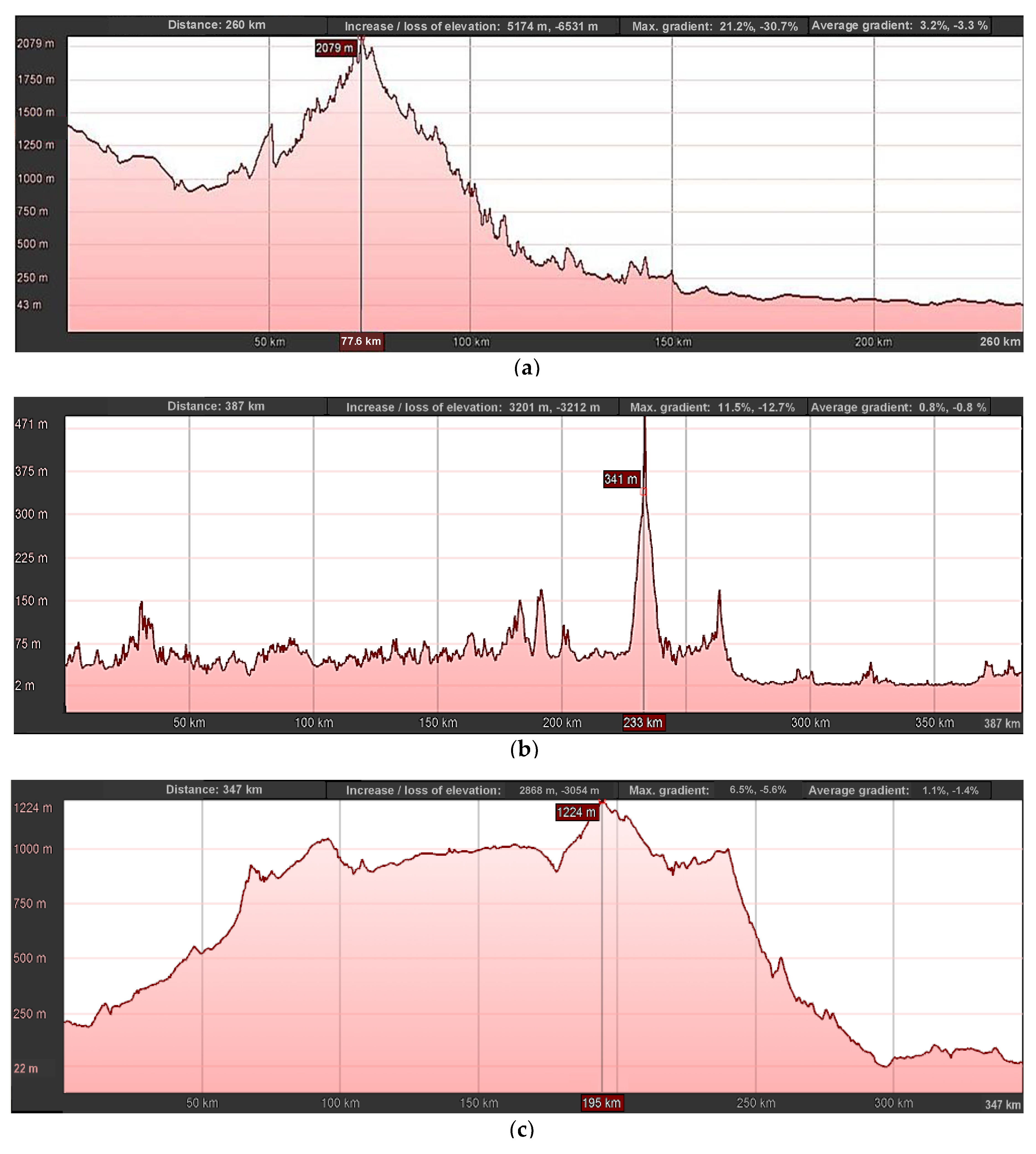
The application of the proposed method for the accounting of TTW emissions for road freight services in the three different locations demonstrates the increase in the accuracy and reliability of this type of calculation through route sections, especially in roads on rugged terrains and with high gradients as in the assessed case in Colombia. In this analyzed service in Colombia, the use of Tier 2 fuel consumption and emission factors from databases or generic tools, developed with data for standard conditions in European or North American countries, generated very high uncertainties when they were applied in different geographies. The diesel consumption on mountainous roads for a fully loaded rigid truck in Colombia was 45 L/100 km, compared to averages between 22–26 L/100 km that are usually applied from other sources. In contrast, the diesel consumption for an articulated truck on a hilly road in Spain from both the proposed method and generic databases coincided with an average of 31 L/100 km. These figures coincided with the average European road type, with traffic at a speed limit of 90 km/h, which is why this journey obtained a similar fuel consumption to the average calculated for the factors in Tier 2. The estimated figure through the Tier 3 method by sections was the closest to the average for this route, which can vary up to 5%, according to the company’s technical director. It is noteworthy that the average consumption for trucks in Europe varies only approximately 10% between a flat and a mountainous road [87] due to the developed infrastructure with several tunnels and viaducts, something nonexistent for the analyzed route in Colombia between two capital cities. In this route, trucks must travel the Western mountain range on narrow roads with fog, sharp curves, high gradients, and unpaved or damaged sections due to landslides. For this reason, the distance of the analyzed route could be done in approximately 4 h in Europe, while the Pereira–Quibdo route takes more than 8 h. In the case of Malaysia, the fuel consumption figures obtained by both the Tier 2 and Tier 3 methods by sections were very similar, but both were also below the actual average for the route. This uncertainty could be produced mainly because none of the methods can account for the extra consumption in dense traffic conditions in urban areas, a variable that affected the analyzed service given that the truck must cross Kuala Lumpur City from south to north through streets with very dense traffic.

The results through the Tier 3 method by sections, despite being closer to the actual consumption than the results obtained with the Tier 2 and Tier 3 method for the entire journey, might have omitted the additional consumption that is generated in the gear shift on each of the slopes in each section, plus many of these slopes have gradients above the average gradient of each analyzed section. On the other hand, the method does not consider the altitude, the age of the truck, or the driving style, factors that significantly influence the actual fuel consumption [6,88,89,90,91]. It is estimated that an efficient driving style can save on average between 5 and 12% [92], and even up to 25% of fuel [93].

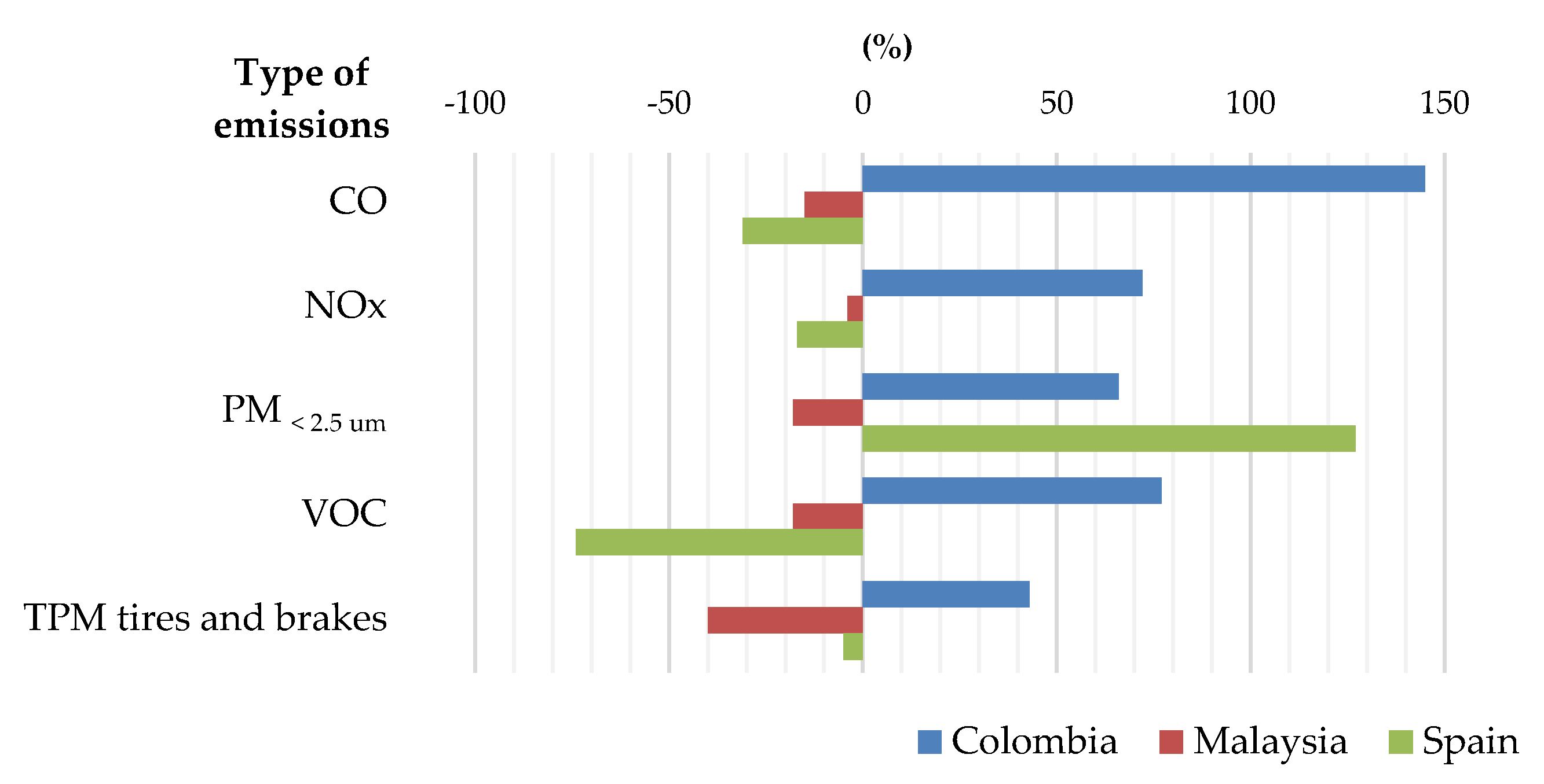
For the assessed case in Spain, due to the similarity in fuel consumption estimations from both the Tier 2 and Tier 3 methods, it could be thought that the use of Tier 2 factors for the estimation of emissions from vehicle operation could be acceptable. However, there are emissions that greatly vary depending on operating parameters, such as air pollutants and tire and brake abrasion emissions. This was demonstrated by the proposed calculation method by sections, where for the loaded truck for the outward journey, a consumption of 35.7 L/100 km was obtained compared to the return of 26.6 L/100 km, which indicates that the quantity of released polluting gases can also vary significantly in each journey. Analyzing the variation rate in the generation of air pollutants obtained by the Tier 3 method by sections compared to the Tier 2 method, very significant changes of up to 145% can be observed in Figure 4.

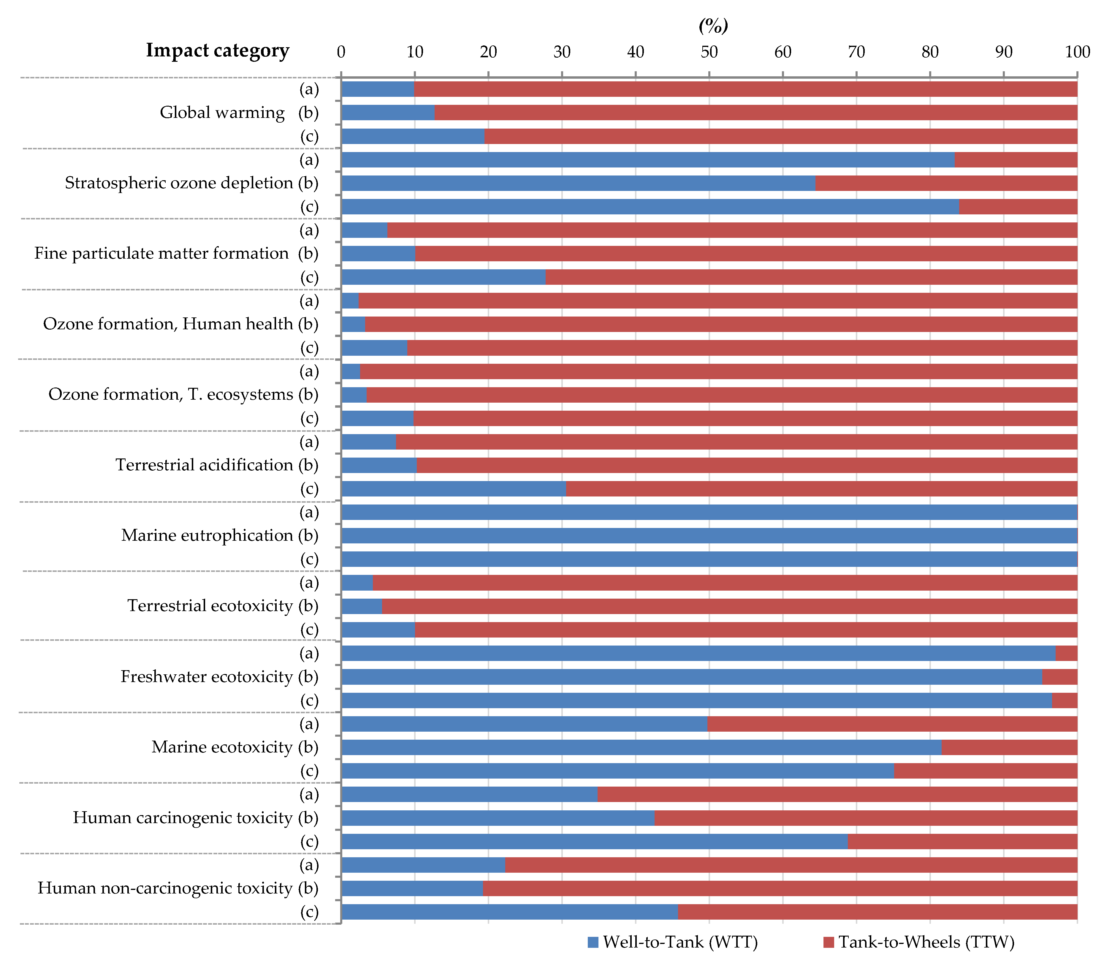
Although the obtained figures from the three studied cases should not be compared, basically because in one of them only the outward journey was considered, and in the other cases, the type of vehicles and load factors were different, important conclusions can be obtained from the analysis of the contribution shares of each phase of the WTW analysis. In general, the environmental impact of the TTW phase was an order of magnitude higher than that of the WTT, so the models used to estimate the corresponding emissions must be as reliable as possible if they are to be used as planning tools or for the environmental reporting of freight transport services.

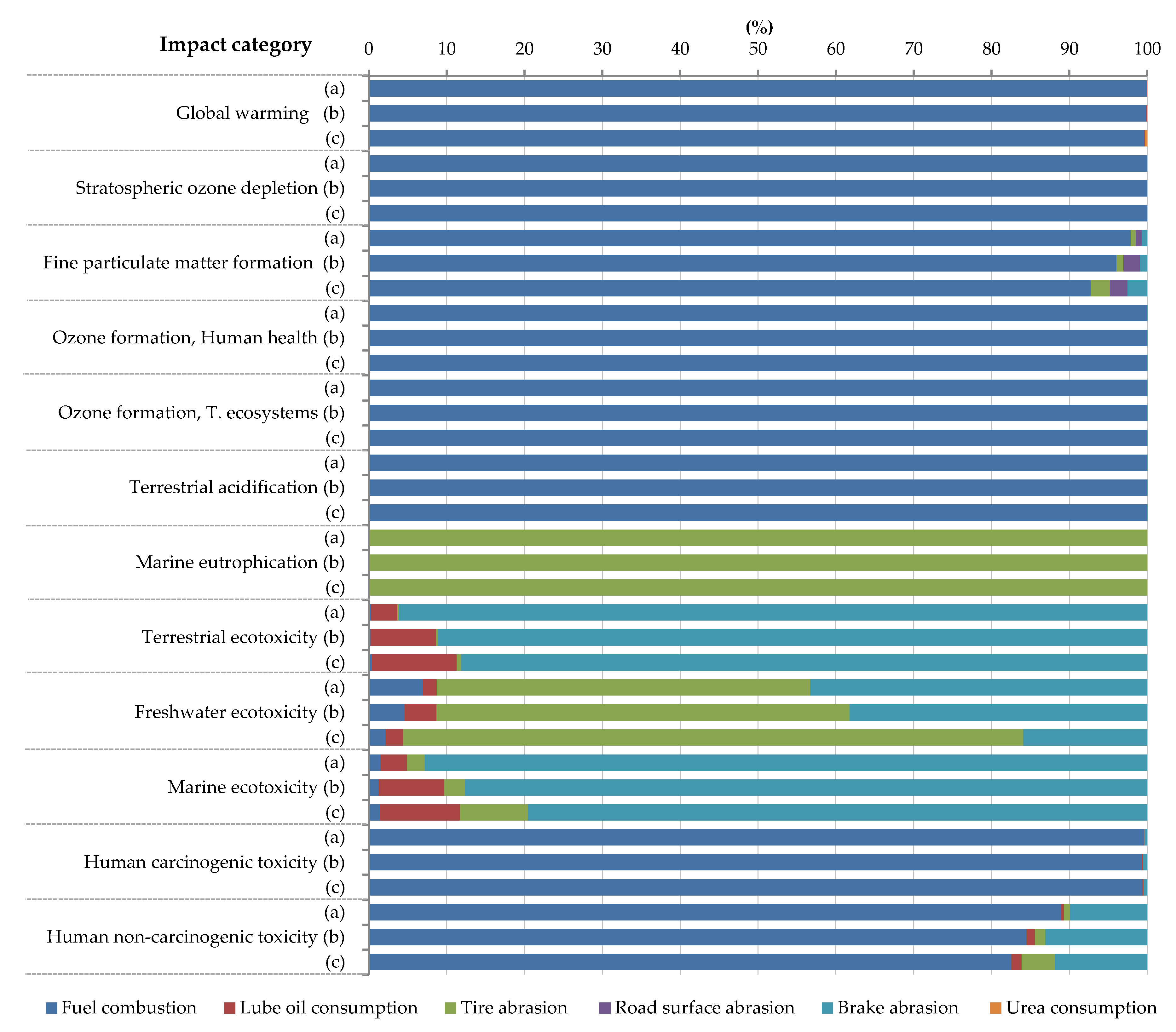
In particular, for all three cases, the TTW phase mainly affected the impact categories related to human health and ecosystems, while the WTT phase affected the categories related to resource availability. The contribution of each phase to the impact categories was mainly influenced by the type of road and by the emission control technology of the vehicle. This can be observed in Spain where the route was carried out by motorway and with a Euro VI vehicle, hence the TTW phase had greater responsibility in seven of the 18 impact categories, compared to the case in Colombia where this phase had responsibility in nine impact categories and with very high contributions, especially in the categories of ozone and particulate matter formation and in human toxicity. Additionally, in the Colombian case, the TTW contribution share was about 50% in marine ecotoxicity impacts, in contrast to shares of 18% and 25% for the Malaysian and Spanish cases, respectively. The high contribution in marine ecotoxicity due to the vehicle operation in the Colombian case was because of the high copper emissions from brake abrasion, which was influenced by the high load factor and low average speed on the mountainous road, generating around three times more brake abrasion particles than those generated in the Malaysian and Spanish cases.

It can also be observed that in each case, there were different contributions in the climate change category, which was not influenced by vehicle technology, but was affected by the fuel production process in each country. In the case of Spain, the WTT phase for B5 diesel at the station generated 0.74 kg CO₂ eq/kg, compared to 0.32 kg CO₂ eq/kg of B10 diesel in Colombia and 0.43 kg CO₂ eq/kg of B7 diesel in Malaysia; which means GHG emissions of 17.3, 7.5, and 10 g CO₂ eq/MJ, respectively. This is because the ULSD in Spain needs higher energy expenditure than the conventional diesel production used in Colombia. Additionally, the electricity used in Colombia is 76% produced by hydroelectric power [94], contributing less CO₂ to the process. Furthermore, the petroleum used in Spain is transported from different continents, compared to the local petroleum used in Colombia. In addition, there is a very important factor that increases the amount of CO₂ to each kg of B5 diesel in Spain, which is related to the production of palm oil biodiesel. In the case of Colombia, the 10% of palm oil biodiesel in the fuel generated a reduction of CO₂ emissions in this WTT phase. However, the 5% of biodiesel incorporated in the fuel in Spain increased the CO₂ emissions by more than 30%. This is because the palm oil production in Malaysia and, mainly in Indonesia, has been grown in tropical forests and peatlands, whose preparation for cultivation releases large amounts of CO₂ [95,96]. In consequence, the total GHG, including combustion emissions, were 88.5, 75.6, and 78.5 g CO₂ eq/MJ of B5, B10, and B7 diesel in the respective countries. Despite this environmental impact of fuel in Spain, the use of Euro VI vehicles and ULSD achieved relatively low impacts against cases, such as Colombia, in the categories related to human health. For example, WTW emissions for the categories of fine particulate matter formation, ozone formation, and terrestrial acidification per km, in the case of Spain, were 1.26 g PM_2.5 eq, 5.80 g NOx eq, and 3.08 g SO₂ eq, respectively, when compared to 15.8 g PM_2.5 eq, 16.1 g NOx eq, and 7.38 g SO₂ eq in the studied case in Colombia, which shows the importance of fuel and vehicle emissions regulations.

The application of the Tier 3 method for the estimation of emission factors is considered a reliable method since for diesel heavy vehicles, the data has been based on a sufficiently large set of experimental data [55]. However, in addition to the experiments that have been conducted under European driving conditions, these factors did not consider the error caused by the mileage age of the vehicles and the cold-start overemissions, therefore, increasing the uncertainty for all estimated gases, especially for CO and VOC emissions. To verify the uncertainty of the obtained estimations, basically, a soft verification method was used by comparing the estimations with the results from the Tier 2 factors and other GHG calculation tools. A ground truth verification method was applied only for the fuel consumption figures due to the impossibility of applying on-board measurements since two of the tested vehicles had pre-Euro and Euro I technology, which lacked on-board diagnostic (OBD-II) connectors for the use of instrumentation for the collection of operation data, consumption, and emissions during the journeys, being practical and necessary for the theoretical estimation by the proposed method for companies that have these types of old technology vehicles. Another parameter that can change the uncertainty in the estimations is the average speed caused by dense traffic, heavy meteorological conditions, or incidents on the road, such as landslides or accidents. This parameter more significantly affected freight transport on single lane roads on mountainous topology than on motorways. In this sense, a sensitivity analysis of the freight transport in the Colombian case was conducted for three scenarios: A fast service where the journey time was reduced by half an hour in optimal road conditions and low traffic; a slightly delayed service, which lasted half an hour more due to the traffic; and a very delayed service that could take up to two hours more due to heavy rain conditions. In the fast service scenario, due to the reduction of 6–7% in the journey time, the fuel consumption and the respective fuel-dependent emissions were reduced by 3.4%, while the emissions of air pollutant gases were reduced between 2.4% and 9%. In the slightly delayed service, the 6–7% increased time produced an increase of 3.9% in fuel consumption and fuel-dependent emissions, and between 3% and 11% of the air pollutant emissions. In the 2-h delay scenario, the 23% increased time produced an increase of 17% in the fuel consumption and fuel-dependent emissions, and between 12% and 47% of the air pollutant emissions. These assessed scenarios show that variation in the journey time and, consequently, the average speed does not cause a direct proportional variation in the fuel consumption and emissions. This is mainly because the fuel consumption and emissions are more affected by other parameters, such as the road section gradients. For this reason, to increase the accuracy of the results, it is important to elaborate new estimations by applying the proposed method every time a freight service parameter changes, since extrapolating previously calculated average emission factors could increase the uncertainty in the results.

5. Conclusions

The proposed emissions estimation method in this paper, unlike most similar methods where only the type of vehicle and the emission control technology are considered, also considers the load factor, gradients, and speed for the different slopes that can be found on a specific route. Through this method, companies, in addition to being able to estimate GHG emissions for journeys in which fuel consumption is unknown, can estimate other emissions, such as air pollutant gases and particles from the abrasion of tires, brakes, and road surface. From these estimations, companies can calculate the carbon footprint of the transported products as well as analyze the different environmental impacts related to the operation of the vehicle and the corresponding fuel used for a specific route. From these analyses, measures can be taken to reduce the impacts of the operation, such as load limits, speed, fleet modernization, or change of type and fuel supplier. It is worth mentioning that this estimation method by sections of the route, supported by information of open source software for the elaboration of elevation profiles, is mainly useful for small and medium companies with limited resources to establish environmental accounting through tools or commercial equipment, which are commonly not adapted to the actual conditions of their operation.

The results of the case studies showed the high uncertainties by using fuel consumption and emission factors from databases developed in a different region to where the freight service took place. Specifically, the diesel consumption on mountainous roads in Colombia was 45 L/100 km, compared to averages between 22–26 L/100 km from generic factors from European sources. In contrast, the diesel consumption for an articulated truck on a hilly motorway in Spain from both the proposed method and generic factors coincided at 31 L/100 km, because this route has similar characteristics to the average European road type and driving conditions. However, even for the Spanish route, the estimated air pollutant emissions by the proposed method differed up to 127% when compared to the generic factors, since the vehicle speed, load, and road gradient have a relevant impact in these emissions. Similarly, for the Colombian route, the variation in air pollutant estimations was up to 145%, while the Malaysian route was up to 40%. The differences in the obtained results in each country were basically because of the topology and characteristics of the roads and the emission control technologies of vehicles. In general, the consideration of air pollutants and tire, brake, and road surface emissions and specific parameters of the operation revealed the importance of emission sources other than diesel combustion and different impact categories to climate change. Specifically, we can highlight the impact generated by the vehicle operation in the terrestrial and marine ecotoxicity categories, where the main reason is the released copper particles by the brake abrasion. The results also showed that the fuel consumption and emissions, depending on the type and condition of the road, could increase more than double when compared to a motorway in good condition. It can be seen that the more rugged the terrain, the greater the variation of non-dependent gases on fuel consumption considering the different operating parameters when compared to the average Tier 2 emission factors, which were established according to the type of vehicle and the emission control technology. In this sense, the investment made in the construction of infrastructure, despite generating environmental impacts, can generate reductions in vehicle operation that would compensate for the impacts in some of the assessed categories. Therefore, it is interesting to include infrastructure construction processes in the life cycle analysis associated with transport services.

In conclusion, the relevance of the different emission sources that must be taken into account was demonstrated, being necessary to apply estimation methods for specific sections of the route, given that the quantity of pollutant emissions is extremely influenced by the speed, load factors, and road gradients. These factors are decisive when evaluating the environmental impacts associated with a specific transport service and the various strategies that are intended to be implemented to improve the sustainability of the sector in different territories.