Spatial-Temporal Changes of Soil Respiration across China and the Response to Land Cover and Climate Change

Abstract

Soil respiration (Rs) plays an important role in the carbon budget of terrestrial ecosystems. Quantifying the spatial and temporal variations in Rs in China at the regional scale helps improve our understanding of the variations in terrestrial carbon budgets that occur in response to global climate and environmental changes and potential future control measures. In this study, we used a regional-scale geostatistical model that incorporates gridded meteorological and pedologic data to evaluate the spatial Rs variations in China from 2000 to 2013. We analysed the relationship between Rs and environmental factors, and suggest management strategies that may help to keep the terrestrial carbon balance. The simulated results demonstrate that the mean annual Rs value over these 14 years was 422 g/m²/year, and the corresponding total amount was 4.01 Pg C/year. The Rs estimation displayed a clear spatial pattern and a slightly increasing trend. Further analysis also indicated that high Rs values may occur in areas that show a greater degree of synchronicity in the timing of their optimal temperature and moisture conditions. Moreover, cultivated vegetation exhibits higher Rs values than native vegetation. Finally, we suggest that specific conservation efforts should be focused on ecologically sensitive areas where the Rs values increase significantly.

1. Introduction

Soil respiration, Rs, is the primary path by which CO₂ fixed by land plants returns to the atmosphere and is the main contributor to terrestrial ecosystem respiration [1,2]. Rs, which is estimated to range from 68 to 98 Pg C/year globally, is the second-largest terrestrial carbon flux; thus, it plays an important role in the carbon budget of terrestrial ecosystems [3,4,5,6]. Rs is sensitive to climatic factors (e.g., temperature and precipitation) [1,5,7] and land cover [8,9]. Hence, it is substantially impacted by global climate and environment changes [10,11].

Previous studies have typically focused on the calculation of Rs and the analysis of its variations at different spatiotemporal scales. At field scale, quite a few studies [12,13,14] have examined the spatial and seasonal variations in Rs using field measurements to assess the dynamic behaviour of Rs. At regional scale, Reichstein et al. (2003) developed a temperature, precipitation and leaf area index (T&P&LAI) model that describes the seasonal and interannual variability in Rs in Europe and North America from 1999 to 2002 [15]. At the global scale, Raich et al. (2002) used a climate-driven temperature and precipitation (T&P) regression model to evaluate the monthly and interannual variations in Rs from 1980 to 1994 [5]. Hashimoto et al. (2015) developed a semi-empirical climate-driven model of Rs by modifying and updating Raich’s model [6]. Bond-Lamberty and Thomson (2010) analysed a compilation of published studies to construct a global Rs database spanning the measurement years 1961–2008 [16].

It has long been demonstrated that temperature and precipitation are two of the main environmental factors in different ecosystems that affect Rs and the effects are nonlinear and synergistic [15,16,17]. In general, temperature is the dominant control over Rs [18,19]. Precipitation is an important driver over Rs when it comes to a water-limited ecosystem [18,20,21,22]. Furthermore, other environmental factors can create synergistic effects with temperature and precipitation on Rs. Different land covers can alter ecosystems through modifications of surface and air temperature, biota and hydrologic routing [23]. The vegetation cover, microbial activities and biological crust cover can change the temperature sensitivity of Rs [15,19,24,25,26]. In addition, a number of studies have investigated methods for reducing anthropogenic impacts on Rs to maintain the terrestrial carbon balance [1,22,23,27,28].

China has the third-largest land area of any country in the world, and it contains diverse climate zones [29] and land-cover systems [30]. Quantifying the spatial and temporal variations in Rs in China is of great significance in understanding the variations in terrestrial carbon budgets that occur in response to global climate and environmental changes and potential future control measures. In the past decades, many studies have assessed Rs in China [31,32,33,34]. In spatial terms, by applying process-based or geostatistical models, these studies use gridded data to simulate the spatial distribution of Rs within China as a whole or particular regions in China [32,35]. Temporally, by calculating the interannual mean Rs values for entire regions, they analyse the trends in Rs revealed by time series [34,36]. However, few studies combine spatially gridded data and time series data to perform deep analyses of variations in Rs.

In terms of the mechanisms by which Rs varies, many insights have been obtained at the local scale. Many environmental factors are involved, including climatic, pedologic, vegetational and anthropogenic factors [37,38,39,40,41]. In contrast, many fewer studies have been conducted at the regional scale. Yu et al. (2010) described the spatial pattern of Rs in China and its interannual and seasonal variations and provided a brief analysis of the Rs values under different land cover types [33]. Chen et al. (2012) analysed the relationship between interannual variability in Rs and climatic factors (air temperature and precipitation) [34]. However, studies that focus on the relationship between spatial-temporal changes in Rs across China and its diverse climate zones, as well as its various land-cover systems, are still lacking. In addition, the time periods covered by most current studies are concentrated in the last century or at the beginning of this century [5,33,42,43]. In the past decade, extreme weather events have occurred all over China. Examples include Super Typhoon Saomai in 2006, the great floods of the Huaihe River in 2007, and the droughts that occurred in southwestern China in 2009. Meanwhile, China has enjoyed a very substantial economic boom and dramatic expansion of construction land spreading from the east to the west [44,45,46]. Therefore, evaluations of Rs need to be updated to reflect the current situation in China.

Overall, this study will fill the gaps discussed above. The objectives of this study are as follows. (1) Simulate the distribution of RS in China from 2000 to 2013; (2) Use geostatistical methods to analyse the changes in Rs in both the temporal and spatial dimensions; (3) Develop a new statistical perspective to confirm the influence of environmental factors on Rs and attempt to provide some explanation for these links; (4) Suggest management strategies that can be used to maintain the terrestrial carbon balance.

2. Methods

2.1. Data

To permit the use of the Rs model, meteorological data and pedologic data were collected. Meteorological data (precipitation and temperature) measured at 752 national basic meteorological stations in China were obtained from China monthly ground climatic datasets on the China Meteorological Data website (http://data.cma.cn/data/cdcdetail/dataCode/SURF_CLI_CHN_MUL_MON.html). Pedologic data (soil organic carbon, SOC, at a depth of 20 cm) were obtained from the 2nd State Soil Survey. These SOC density data are presented in a vector format at a scale of 1:4,000,000. All of the data above cover the period from 2000 to 2013.

Other environmental variables analysed in this study include climate zones, vegetation and soil types. These terrestrial spatial data, which cover China, were downloaded from the National Earth System Science Data Sharing Infrastructure website (http://www.geodata.cn/). The climate zone data was digitalised from 1:36,000,000 China Climate Zoning Map [47]. The vegetation type data was from the digitalised 1:4,000,000 China Vegetation Type Map [48]. The 1 km × 1 km gridded vegetation map of China includes 6 categories of natural vegetation, 4 categories of cultivated vegetation, and lake regions. Although the vegetation map, which was compiled for past conditions, may not completely match the current vegetation distribution due to the expansion of built-up areas in China, the spatial mismatch in vegetation will not introduce bias into our study because we exclude areas that display changes in land-use type [49]. The 1 km × 1 km soil grid map of China, which represents the genetic classification of the soils, was based on the database obtained from the 2nd State Soil Survey. The soil type data was digitalised from 1:1,000,000 China Soil Map [50].

2.2. Analysis

2.2.1. Calculation of Rs Values

By synthesising the Rs values contained within the ChinaFLUX data set with those published in approximately 200 papers in the literature, Yu et al. (2010) established a Rs database for China and developed a new regional-scale geostatistical model of soil respiration (GSMSR) by modifying a global-scale statistical model. Using 333 Rs observations, the established model has been validated with 57 Rs observations that were not used in the calibration of the model [33]. The GSMSR model, which is driven by monthly air temperature, monthly precipitation, and SOC density, displays improved simulation results within China; thus, we use this model on the annual scale. The model can be written as

$$\mathrm{Rs}=\left(0.588+0.118\times \mathrm{SOC}\right)\times {\mathrm{e}}^{\ln \left(1.83\times {\mathrm{e}}^{-0.006\mathrm{T}}\right)\times \mathrm{T}÷10}\times \left(\mathrm{P}+2.972\right)÷\left(\mathrm{P}+5.657\right)\times 365$$

(1)

where T is the annual mean air temperature (°C), P is the mean monthly precipitation (cm), and SOC is the topsoil (0–20 cm) organic carbon storage density (kg C/m²). An interpolation method was used to generate precipitation and temperature maps, and the inverse distance weighted (IDW) method [51] was used to complete the interpolation to 1 km × 1 km grid layers. The gridded SOC density data at a depth of 20 cm (1 km × 1 km) were obtained based on interpolation from the vector-based 1:4,000,000-scale SOC density data.

2.2.2. Analysis of the Trends in Rs

We use a simple linear regression analysis model of the slope to perform our trend analysis, which combines the spatially gridded data and time series data to obtain gridded time series data [52,53]. This model can be written as follows:

$$\mathrm{slope}=\frac{\mathrm{n}\times {\sum }_{\mathrm{i}=1}^{\mathrm{n}}\mathrm{i}\times {\mathrm{Rs}}_{\mathrm{i}}-{\sum }_{\mathrm{i}=1}^{\mathrm{n}}\mathrm{i}{\sum }_{\mathrm{i}=1}^{\mathrm{n}}{\mathrm{Rs}}_{\mathrm{i}}}{\mathrm{n}\times {\sum }_{\mathrm{i}=1}^{\mathrm{n}}{\mathrm{i}}^2-{\left({\sum }_{\mathrm{i}=1}^{\mathrm{n}}\mathrm{i}\right)}^2}$$

(2)

where slope is the Rs trend, which refers to the general tendency of changes in Rs; n is the number of time intervals (years) studied; Rs_i is the annual Rs for year i; and slope > 0 and slope < 0 represent the increasing and decreasing tendencies of Rs, respectively. To assess the validity of the model, the p-test was used to test the significance, and the tendencies were classified into 5 categories: Highly significant (-) (slope < 0 and p < 0.01), significant (-) (slope < 0 and 0.01 ≤ p < 0.05), no significant change (p ≥ 0.05), significant (+) (slope > 0 and 0.01 ≤ p < 0.05), and highly significant (+) (slope > 0 and p < 0.01).

The trend analysis for each grid cell was carried out by writing code in Matlab.

2.2.3. Correlation Analysis between Rs and Temperature or Precipitation

The Pearson correlation coefficient (R) was employed to present the trend of the Rs with different climate factors (temperature and precipitation), grid by grid. A high R-value indicates a better relationship, while a low R-value represents the opposite. A positive R implies that the Rs has the same trend as a factor, while a negative R implies the opposite. The general level of significance, P value, was taken as 5%. Both the trend and correlation analysis for each grid are finished using Matlab software.

3. Results

3.1. The Distribution of RS and Its Changes across China

Statistically, the 14-year mean annual Rs ranges from 412 to 432 g/m²/year over China as a whole (Figure 1). The mean value of this quantity for all of the grid cells is 422 g/m²/year. Figure 2 shows that Rs decreases from southeast to northwest, but some unusually high values occur in the Qinghai-Tibet Plateau and Taiwan.

Temporally, the total annual Rs displays a wide range between 115 and 3260 g/m²/year from 2000 to 2013 in each grid cell across China (Figure 2). The total annual Rs value fluctuates between different years, but shows a slightly increasing trend on the whole (Figure 1). The coefficient of variation shows a slight decline during the 14 years, and it peaks in 2001 and dips in 2007.

A grid cell-based trend analysis (Figure 3) shows that the Rs changed from −14.02 to 18.23 g/m²/year, and the mean annual increasing slope is 0.31 g/m²/year on the whole. Many more grid cells show increasing trends, and these cells account for 70.69% of the total number. The grid cells that display increasing trends show a mean increasing slope of 0.75 g/m²/year, and these grid cells are distribute along the northeastern edge of the Qinghai-Tibet Plateau and are scattered throughout parts of northeastern and southern China. On the other hand, for the grid cells that display decreasing trends, the mean decreasing slope is −0.75 g/m²/year, and these cells are concentrated in southwestern China and along the Yangtze River. Furthermore, we performed a significance test of the annual Rs trends from 2000 to 2013 (Figure 4). The highly significantly decreasing and significantly decreasing grid cells account for only 0.11% and 0.70% of the total number of grid cells, respectively, whereas the highly significantly increasing and significantly increasing grid cells account for higher percentages of 3.49% and 6.59%, respectively. These grid cells are located in the eastern Qinghai-Tibet Plateau and parts of northwestern China.

The labels highly significant (+), significant (+), non-significant (+) and (-), significant (-) and highly significant (-) indicate that an increasing trend in Rs is significant at the 99% or 95% confidence levels; that an increasing or decreasing trend is non-significant; or that a decreasing trend is significant at the 99% or 95% confidence levels, respectively.

3.2. Correlation Analysis between Rs and Temperature Or Precipitation

We perform a correlation analysis between Rs and temperature on a per-grid-cell basis (the results are shown in Figure 5a). Up to 62.91% of the grid cells display significant positive correlations between Rs and temperature. These grid cells have a mean R value of 0.51 and p values < 0.05. In addition, none of the grid cells display significant negative correlations. Spatially, strong correlations exist in northwestern China, and no consistent relationship between Rs and temperature is seen in northern and southeastern China.

We also perform a correlation analysis between Rs and precipitation on a per-grid-cell basis (the results are shown in Figure 5b). Approximately 59.92% of the grid cells display significant correlations between Rs and precipitation. These grid cells have p values < 0.05. Of these grid cells, 99.96% display positive correlations, and the mean R value is 0.54. The grid cells with strong correlations are spread across northern and southeastern China. No consistent relationship between Rs and precipitation exists in western or northeastern China.

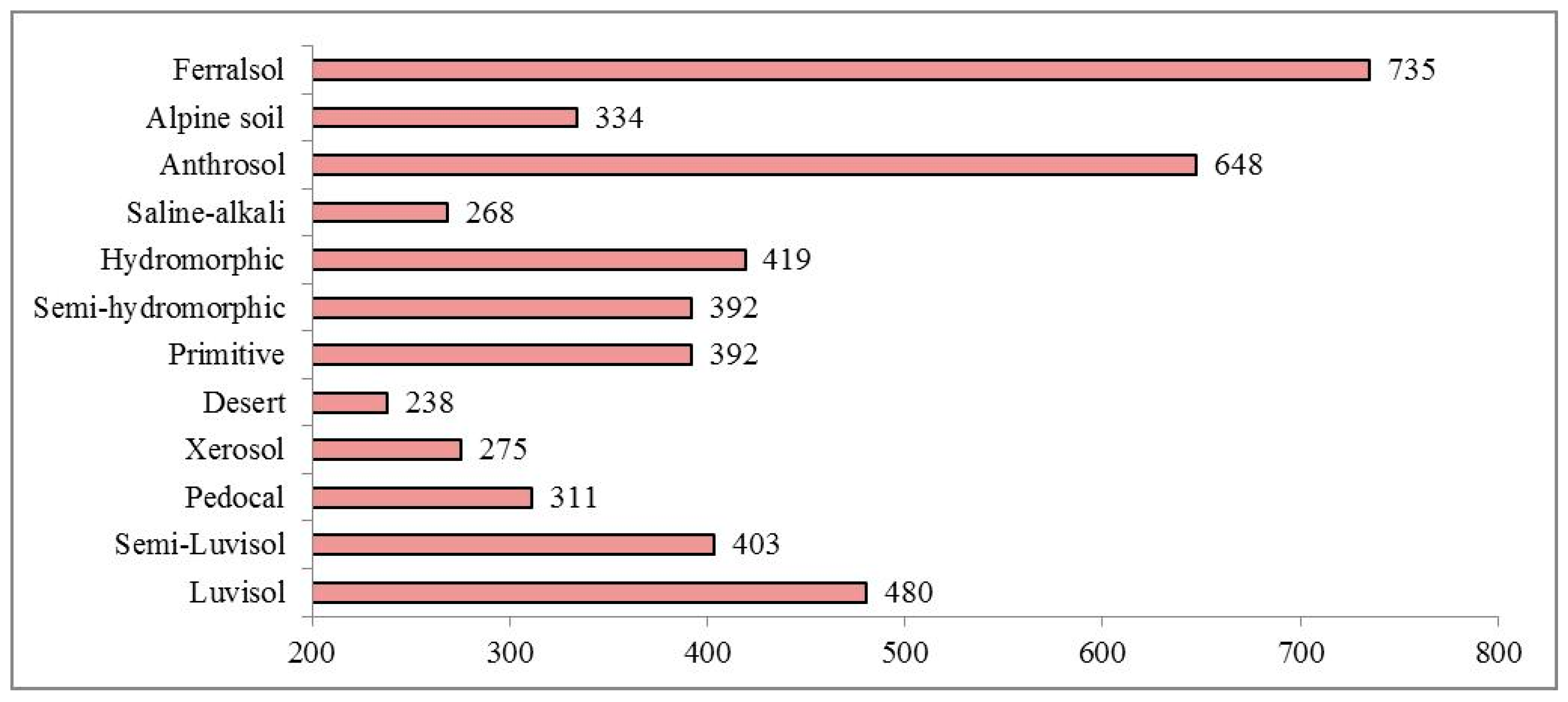
3.3. Rs Values in Different Climate Zones, Land-Use Types and Soil Types

Statistics of Rs values for different climate zones are shown in Figure 6. The value of Rs in the tropical monsoon climate zone (846 g/m²/year) is highest among the five climate zones, whereas the value of Rs in the temperate continental climate zone (266 g/m²/year) is lowest. In terms of interannual variability, calculation of the coefficient of variation shows that the yearly changes in Rs in the temperate monsoon climate zone are greater than those in any other climate zone. On the other hand, Rs displays smaller yearly changes in the subtropical monsoon climate zone. Furthermore, the grid cell-based trend analysis shows that, for the values of Rs in the five climate zones, only the subtropical monsoon climate zone displays a decreasing trend. In addition, of the other four climate zones, an increasing trend is most evident in the alpine climate zone, especially in the eastern portion of the Qinghai-Tibet Plateau. Spatial distribution of different climate zones in China is seen in Figure 7.

The Rs values also differ among the land-use systems (Figure 8). In terms of the two largest-scale groups, native vegetation and cultivated vegetation, the latter exhibits higher Rs values. Given a finer breakdown into 11 different land-use systems, double-cropped paddy field-dominated vegetation has the highest mean value (819 g/m²/year), whereas desert vegetation presents the lowest mean value (245 g/m²/year). Moreover, desert vegetation also displays the greatest variability in its value during the 14 years. The shrub and coppice land-use types tend to display relatively little interannual variability. Based on the grid cell-based trend analysis, all of the land-use systems, except for mixed cropland that is harvested twice a year and double-cropped paddy field-dominated vegetation, display increasing trends in Rs. Of the land use systems, the mean annual increasing slope of meadow and herbaceous swamp is 0.97 g/m²/year, which is the highest value on the list. On the other hand, for the grid cells that display decreasing trends, the mean annual slope of mixed cropland with two harvests a year (−0.94 g/m²/year) is lower than that of double-cropped paddy field-dominated vegetation (−0.38 g/m²/year).

The Rs values also differ among the soil types (Figure 9). Of the 12 soil orders, the ferralsols display the highest Rs values; the anthrosols and luvisols display the next highest Rs values; and the desert soils, saline-alkali soils and xerosols exhibit the lowest Rs values. In terms of interannual variability, all of the 12 soil orders show small yearly changes, and the corresponding coefficients of variation are less than 0.03.

3.4. Cross Analysis of Climate Zones and Land-Use Types in Terms of Their Rs Values

Using a pivot chart of the mean values (Figure 10a) and the coefficients of variation (Figure 10b), we also compare the Rs values for the different land-use types within particular climate zones and vice versa.

For the tropical monsoon climate zone and temperate continental climate zone, the variance in the Rs values is similar among the different land-use types and stable for the individual types. For the subtropical monsoon climate zone, the Rs values are the highest in double-cropped paddy field-dominated vegetation and lowest in dry cropland-dominated vegetation that is harvested once a year. The Rs values in areas of meadow and herbaceous swamp clearly show greater variation than any other land-use type. For the temperate monsoon climate, we determine that the Rs values are the highest in mixed cropland with two harvests a year and the lowest in desert vegetation. For the alpine climate zone, the highest Rs values are identified in coniferous forest and lowest in desert vegetation. For all of the climate zones, except for the tropical monsoon climate, where no data are available, the Rs values in meadow and herbaceous swamp clearly show greater variability than those of any other land-use type.

For all of the land-use types (except for types with no data), the Rs values in the tropical and subtropical monsoon climate zone are higher than those of the other climate zones; meanwhile, the lowest Rs values consistently appear in the temperate continental climate zone. In terms of the variation in Rs values, the Rs values within the alpine climate zone are generally more unstable than those in any other climate zone. On the other hand, in the monsoon climate zone, the Rs values usually change only slightly.

4. Discussion

4.1. Model Validation and Comparison of Rs Evaluations Presented by Different Studies

The model we used to simulation Rs was developed on large field observations in China by Yu et al. 2010, and it has high accuracy to be used in China. In this study, we also collected and updated up to 66 field-observed Rs data to test its applicability. The data includes China’s main ecosystems, of forest, grassland, cropland and wetland in different parts of China (

Table 1. Rs field studies done at different parts of China (Rs g/m²/year).

ID	Latitude	Longitude	Year	Vegetation	Field-Observed Rs	Model-Calculated Rs	Precision
1	29.68	91.35	2000	Cropland	579.00	584.20	99.10%
2	34.27	108.08	2001	Cropland	425.80	433.92	98.09%
3	29.67	91.33	2000	Cropland	579.00	590.97	97.93%
4	47.10	126.13	2007	Cropland	517.17	467.81	90.46%
5	35.07	113.17	2002–2004	Cropland	286.17	338.30	81.78%
6	28.92	111.45	2003	Cropland	554.30	663.50	80.30%
7	36.93	114.60	2004	Cropland	648.78	428.55	66.05%
8	26.80	109.50	2003	Forest	526.00	709.480	65.12%
9	26.73	115.07	2004	Forest	554.00	708.67	72.08%
10	23.17	112.53	2003	Forest	863.30	839.54	97.25%
11	31.32	110.50	2009	Forest	627.00	644.86	97.15%
12	23.17	112.53	2003	Forest	866.00	839.54	96.94%
13	31.33	110.50	2009	Forest	624.00	643.93	96.81%
14	31.27	105.47	2005	Forest	511.30	527.87	96.76%
15	21.93	101.25	2008	Forest	780.00	814.56	95.57%
16	21.93	101.27	2004	Forest	885.00	796.58	90.01%
17	21.95	101.20	2003	Forest	742.00	822.29	89.18%
18	44.00	88.00	2005	Forest	262.50	291.13	89.09%
19	31.32	110.48	2009	Forest	580.00	645.01	88.79%
20	26.73	115.07	2005	Forest	632.00	718.66	86.29%
21	42.40	128.47	2002	Forest	503.00	429.92	85.47%
22	26.19	117.43	2003	Forest	829.30	693.31	83.60%
23	21.85	101.20	2008	Forest	1007.00	815.03	80.94%
24	31.58	102.58	2008	Forest	960.25	775.59	80.77%
25	31.27	105.45	2005	Forest	655.00	527.51	80.54%
26	26.22	117.53	2002	Forest	924.00	742.99	80.41%
27	23.18	112.55	2003	Forest	1053.00	839.47	79.72%
28	23.18	112.54	2003	Forest	1055.00	839.50	79.57%
29	27.50	114.50	2006	Forest	975.96	747.91	76.63%
30	26.20	117.43	2001	Forest	960.33	730.31	76.05%
31	26.18	117.47	2012	Forest	906.46	680.03	75.02%
32	26.19	117.43	2002	Forest	1018.70	743.64	73.00%
33	22.68	112.90	2004	Forest	1162.00	840.33	72.32%
34	30.23	119.70	2013	Forest	1015.91	724.22	71.29%
35	41.90	124.90	2006	Forest	498.32	346.42	69.52%
36	30.30	103.00	2008	Forest	592.00	406.85	68.73%
37	30.50	103.00	2004	Forest	884.94	603.65	68.21%
38	26.73	115.07	2004	Forest	537.00	712.20	67.37%
39	28.12	113.03	2007	Forest	496.00	673.99	64.11%
40	42.40	128.10	2004	Forest	684.32	428.60	62.63%
41	28.12	113.03	2008	Forest	488.00	678.74	60.91%
42	26.32	117.60	2012	Forest	1232.59	737.60	59.84%
43	23.17	112.17	2005	Forest	627.80	881.91	59.52%
44	23.13	112.59	2002	Forest	1001.00	865.12	86.43%
45	21.93	101.27	2004	Forest	1273.00	813.53	63.91%
46	25.32	110.55	2013	Forest	1160.70	748.90	64.52%
47	30.23	119.70	2013	Forest	1109.00	724.22	65.30%
48	26.18	117.47	2012	Forest	927.20	680.04	73.34%
49	31.30	102.93	2013	Forest	815.50	558.62	68.50%
50	22.17	106.83	2012	Forest	995.50	821.98	82.57%
51	32.18	118.70	2013	Forest	980.00	639.06	65.21%
52	27.67	114.63	2006	Forest	1055.00	633.87	60.08%
53	29.28	115.72	2006	Forest	900.70	679.56	75.45%
54	43.55	116.82	2001–2002 2004–2005	Grassland	314.46	302.48	96.19%
55	44.09	115.91	2002	Grassland	111.00	326.21	93.88%
56	44.75	123.75	2002	Grassland	300.50	272.39	90.64%
57	43.55	116.78	2004	Grassland	356.00	311.84	87.59%
58	44.81	116.26	2011–2012	Grassland	219.45	248.92	86.57%
59	43.55	116.78	2003	Grassland	360.00	305.19	84.77%
60	43.43	116.07	2001–2002 2004–2005	Grassland	263.42	217.32	82.50%
61	43.55	116.78	2002	Grassland	409.00	296.74	72.55%
62	30.85	91.08	2004	Grassland	369.06	242.83	65.80%
63	30.90	91.10	2004	Grassland	369.00	242.73	65.78%
64	44.09	115.91	2003	Grassland	126.00	332.93	64.23%
65	37.58	101.33	2013	Wetland	454.10	517.85	85.96%
66	37.76	118.99	2012	Wetland	794.70	525.47	66.12%

Note: Precision = Abs(1 − Abs(1 − M/F)). M for model-calculated Rs and F for field-observed Rs.

). It shows the precision ranged between 60.08% to 99.1%, with mean value of 79%. Although the amount of observations we collected are not high, since the model itself was developed on large field observations before 2010 in China, the model is also applicable and has high accuracy to be used in China after 2010. Furthermore, we compare our estimated Rs values for the whole China with those produced by different studies [5,33,34,42,43]. The results of this study, which suggest an average of 422 g/m²/year and a total of 4.01 Pg C/year from 2000 to 2013, fall within the results of other models (

Table 2. Rs estimates for China produced by different studies.

Model	Period	Rs (Pg C/year)	Reference
GSMSR	2000–2013	4.01 (3.91–4.10)	this study
GSMSR	1995–2004	3.84 (3.77–4.00)	Yu et al., 2010
T&P&C	1970–2009	4.83 (4.58–5.19)	Chen et al., 2012
T&P	1995–2004	3.51	Yu et al., 2010
T&P	1980–1994	3.76	Raich et al., 2002; Yu et al., 2010
CEVSA	1980–2000	4.82	Cao et al., 2003; Yu et al., 2010
AVIM2	1981–2000	4.43	Ji et al., 2008; Yu et al., 2010

). These values are slightly larger than the estimates produced using the T&P model and the geostatistical model of soil respiration (GSMSR) by Yu et al. (2010). However, these results are lower than the results of the T&P&C model (which uses the mean air temperature, the sum of annual precipitation and soil organic carbon storage as predictors) and two process-based Rs models, specifically the Carbon Exchange between Vegetation, Soil and Atmosphere (CEVSA) model and an atmosphere-vegetation interaction model (AVIM2). However, great uncertainty remains in the estimates of annual soil respiration in terrestrial ecosystems in China, with differences of 1 Pg C/year between the highest and lowest values. We attribute these differences to the spatial and temporal resolutions of environmental variables, the modelling period investigated, and the data used in the parametrisation of the models used.

Compared with other models, the model used in this study and its parameters were validated by Yu et al. (2010), which confirms their appropriateness specifically for China. This study uses uniformly distributed gridded data to evaluate Rs to improve the spatial representativeness of the model. Furthermore, we perform trend analysis and partition calculations for different climate zones and land-use types to promote understanding of Rs variations. The general Rs evaluation in this study does not resolve the specific processes involved in Rs (e.g., heterotrophic and autotrophic respiration), which should be included in future studies to refine the model.

4.2. Spatiotemporal Patterns of Rs and Its Changes across China

In spatial terms, Rs generally decreases from southeast to northwest across China, and this pattern is consistent with the spatial distribution of precipitation. This conclusion agrees with previous studies by Yu et al. (2010) [33]. Although the mean annual air temperature in northwestern China is higher than that in some portions of northeastern China, the greater topsoil organic carbon storage in northeastern China may result in higher annual soil respiration. In contrast, the lower temperature, reduced precipitation and smaller topsoil organic carbon pools in northwestern China produce the lowest annual soil respiration there.

Note that some especially high Rs values are dispersed in the Qinghai-Tibet Plateau and Taiwan, due to the high levels of soil organic carbon (SOC). Overlaying Figure 2 on the grid maps of soil type and vegetation type, we found that high values in the Qinghai-Tibet Plateau are distributed on the swamp, while high values in Taiwan are scattered on yellow brown soils (belonging to luvisol) and in broad-leaved forest. Soils of these regions are probably rich in organic carbon [54,55].

4.3. Effects of Precipitation and Temperature on Rs

Numerous studies indicate that, instead of a linear correlation, there is a complex relationship between Rs and climatic factors (e.g., temperature and precipitation) [1,7,56,57]. We put Figure 5a,b together to explore the influence of temperature and precipitation on Rs in different parts of China. The blue in Figure 5 means where the climatic factor is less important. In northern and southeastern China, precipitation plays a major role; In northwestern and northeastern China, temperature becomes dominant; In central China where transitional, both precipitation and temperature have significant influence; In the Qinghai-Tibet Plateau, neither precipitation and temperature have clear patterns of influence on Rs.

Precipitation is an important factor that influences Rs from 2000 to 2013. Especially in northern and southeastern China, where rainfall is abundant, the Rs values are highly correlated with precipitation. On the other hand, in the areas that lack rain, the Rs values are less strongly correlated. Rainfall controls the spatial and temporal variations in vegetation productivity in the cropland, grassland and forest ecosystems. Specifically, this phenomenon is more obvious in the monsoon climate zone. Vegetation biomass varies greatly with the changes in soil water availability that occur due to precipitation variations. Precipitation may influence soil respiration through changes in vegetation growth and root activity. In this sense, precipitation is an important factor that controls the terrestrial carbon cycle, as the processes that control the inputs of carbon into ecosystems and the outputs of carbon from ecosystems are related to precipitation.

From the spatial distribution of mean annual Rs values, we know that temperature has a less significant effect on Rs than precipitation. It plays a leading role in controlling Rs values only when precipitation is limited, usually in the continental climate zone. Thus, a high correlation between Rs and temperature exists in northwestern China, but there is no consistent relationship between these variables in northern and southeastern China. Nearly all models of global climate change predict a loss of carbon from soils as a result of global warming. Global warming increases soil decomposition where Rs is limited by temperature. Moreover, it accelerates the turnover of carbon in soils, which increases the flux of CO₂ from soils. Moreover, low temperatures suppress the effects of precipitation on Rs. The situation in northeastern China provides an example of this behaviour.

Therefore, high Rs values are seen in areas such as the tropical and subtropical monsoon climate zone. These regions show a greater degree of synchronicity in the timing of their optimal temperature and moisture conditions. In contrast, due to the lack of precipitation and heat, the temperate continental climate zone unsurprisingly displays low Rs values. In addition, given its complex climatic conditions, there are no clear patterns in Rs in the alpine climate zone.

4.4. Effects of Land Use on Rs

Effects of land use on Rs in part reflect the influence of climatic factors on Rs since land use cover is strongly linked to climate at regional scale. Therefore, in this study, double-cropped paddy field-dominated vegetation has the highest Rs mean value and desert vegetation presents the lowest.

The vegetation changes resulting from land-use conversions may directly affect the physicochemical and microbiological properties of soil and thus soil respiration [8,9,58,59,60]. Land-use conversion change root types and biomass, as well as the substrate carbon input and availability, thus indirectly influencing soil respiration [60,61]. Without increasing the stock of soil organic matter, tillage cultivation increases the flux of CO₂ from soils, as the conditions for decomposition—soil aeration and moisture content—are often improved when soils are disturbed, leading to greater rates of soil respiration. Besides, the inputs of fresh plant debris to soils are lower when native vegetation is converted to agriculture. Cultivation also disrupts soil aggregates, exposing stable, adsorbed organic matter to decomposition. That may be the reason why Rs in cultivated vegetation is higher than that in native. Existing agricultural lands are used intensively and efficiently, and the losses of carbon from cultivated soils may be as large as 0.8 × 10¹⁵ gC/year globally [1].

4.5. Effects of Soil Type on Rs

Previous studies indicated that the effects of soil type on Rs can be ascribed to the effects of soil content water, soil temperature, soil organic matter, microbial biomass, soil chemistry and soil physical properties, alone or in combination [62]. The combined effects of soil content water and soil temperature are similar to those of precipitation and temperature on Rs, but these effects occur on a microscopic scale. Soil with too much or too little water content may inhibit the respiration rate. The decreased Rs values that occur at high soil water contents result from reduced oxygen diffusion [12]. Thus, xerosols, desert soils and saline-alkali soils exhibit the lowest Rs values.

Soil texture affects the movement of water and gases in soils and may have profound effects on the efflux rates of CO₂ from soil. The Rs values associated with ferralsols and luvisols are high because they are more porous than other soil types; they have small bulk and particle densities and high porosity. As a result, the diffusion of CO₂ and O₂ is not very easily restricted in these soils, resulting in better aeration and conditions that favour the aerobic decay of soil organic C [63]. Ferralsols and luvisols have high water retention capacities that offer excellent protection against soil drying.

Anthrosols comprises soils that have been formed or heavily modified due to long-term human activities, such as irrigation, the addition of organic waste or the wet-field cultivation used to create paddy fields. The Rs values associated with Anthrosols are high because tillage cultivation increases the flux of CO₂ from soils, as mentioned above.

4.6. Suggested Management Strategies

Based on the analysis above, over 10% of China is experiencing significant or highly significant increases in Rs; thus, greater amounts of CO₂ are released into the atmosphere. To balance the terrestrial carbon budget, we should effectively control the CO₂ flux from soils. Therefore, we should emphasise the application of conservation measures where the Rs values display significant increases. These ecologically sensitive areas are located mainly in northwestern China and around the Qinghai-Tibet Plateau. By overlaying analysis, we can find that these areas are often shrubby or herbaceous without tall trees, or with heavy farm work; the soil in these areas is poor in organic carbon (

Table 3. Land-use types (a) and soil types (b) of areas with highly significant increasing Rs from 2000 to 2013 (over 10%).

a	Land-Use Type	Percentage
	Meadow and herbaceous swamp	21.23%
	Shrub and coppice	20.07%
	Grassland and savanna shrub grassland	16.00%
	Desert vegetation	12.60%
	Mixed cropland with three harvests a year	11.94%
b	Soil Type	Percentage
	Alpine soil	47.26%
	Primitive	13.04%
	Desert	10.65%

). From the discussion above, we confirmed that the CO₂ flux from soils is synthesis process influenced by various environmental factors. Accordingly, protective measures should be comprehensive to adjust the environmental factors. Measures involve (1) fencing and seeding in heavily degraded areas; (2) improving the relevant breeds to control the stocking rates if grazing is necessary; (3) carrying out gully control to reduce soil and water erosion.

In addition, additional attention should be paid to agricultural areas. To reduce the disturbance of soils, we recommend the use of “no-till” agriculture. The institution of no-till techniques on previously cultivated land may actually restore some soil organic matter and inhibit soil respiration. Furthermore, previous studies realise that some of the high rates of carbon sequestration are found when cultivated soils are allowed to revert to native vegetation [1]. Thus, it is necessary to conduct reforestation with native vegetation in sloping or deserted areas which are less desirable for use as cropland.

5. Conclusions

We can conclude that over 10% of China experienced significant or highly significant increases in Rs. The simulated results demonstrate that the mean annual Rs value from 2000 to 2013 is 422 g/m²/year, and the corresponding total value is 4.01 Pg C/year. Rs estimates display a clear spatial pattern decreasing from southeast to northwest.

The estimation indicates that high Rs values may occur in areas that show a greater degree of synchronicity in the timing of their optimal temperature and moisture conditions, although no consistent relationship between Rs and temperature or precipitation exists in some areas of China. The Rs values differ among land use and soil types. Cultivated vegetation exhibits higher Rs values than native vegetation. The effects of soil type on Rs can be ascribed to the effects of soil content water, soil temperature and soil texture. To help to maintain the terrestrial carbon balance, specific conservation efforts should be focused on ecologically sensitive areas where the Rs values increase significantly.

References

1. Schlesinger, W.H.; Andrews, J.A. Soil respiration and the global carbon cycle. Biogeochemistry 2000, 48, 7–20. [Google Scholar] [CrossRef]
2. Coryc, C.; Dianar, N.; Stevenk, S.; Alanr, T. Increases in soil respiration following labile carbon additions linked to rapid shifts in soil microbial community composition. Biogeochemistry 2007, 82, 229–240. [Google Scholar]
3. Schlesinger, W.H. Carbon balance in terrestrial detritus. Annu. Rev. Ecol. Evol. Syst. 1977, 8, 51–81. [Google Scholar] [CrossRef]
4. Field, C.B.; Behrenfeld, M.J.; Randerson, J.T.; Falkowski, P. Primary production of the biosphere: Integrating terrestrial and oceanic components. Science 1998, 281, 237–240. [Google Scholar] [CrossRef] [PubMed]
5. Raich, J.W.; Potter, C.S.; Bhagawati, D. Interannual variability in global soil respiration, 1980-94. Glob. Chang. Biol. 2002, 8, 800–812. [Google Scholar] [CrossRef]
6. Hashimoto, S.; Carvalhais, N.; Ito, A.; Migliavacca, M.; Nishina, K.; Reichstein, M. Global spatiotemporal distribution of soil respiration modeled using a global database. Biogeosci. Discuss. 2015, 12, 4331–4364. [Google Scholar] [CrossRef]
7. Hashimoto, S.; Morishita, T.; Sakata, T.; Ishizuka, S.; Kaneko, S.; Takahashi, M. Simple models for soil CO2, CH4, and N2O fluxes calibrated using a Bayesian approach and multi-site data. Ecol. Model. 2011, 222, 1283–1292. [Google Scholar] [CrossRef]
8. Frank, A.B.; Liebig, M.A.; Tanaka, D.L. Management effects on soil CO2, efflux in northern semiarid grassland and cropland. Soil Tillage Res. 2006, 89, 78–85. [Google Scholar] [CrossRef]
9. Zhang, Y.; Guo, S.; Liu, Q.; Jiang, J.; Wang, R.; Li, N. Responses of soil respiration to land use conversions in degraded ecosystem of the semi-arid loess plateau. Ecol. Eng. 2015, 74, 196–205. [Google Scholar] [CrossRef]
10. Jones, C.D.; Cox, P.; Huntingford, C. Uncertainty in climate-carbon-cycle projections associated with the sensitivity of soil respiration to temperature. Tellus B 2003, 55, 642–648. [Google Scholar] [CrossRef]
11. Trumbore, S. Carbon respired by terrestrial ecosystems—Recent progress and challenges. Glob. Chang. Biol. 2006, 12, 141–153. [Google Scholar] [CrossRef]
12. Xu, M.; Qi, Y. Spatial and seasonal variations of Q, 10, determined by soil respiration measurements at a Sierra Nevadan Forest. Glob. Biogeochem. Cycles 2001, 15, 687–696. [Google Scholar] [CrossRef]
13. Arevalo, C.B.M.; Bhatti, J.S.; Chang, S.X.; Jassal, R.S.; Sidders, D. Soil respiration in four different land use systems in north central Alberta, Canada. J. Geophys. Res. Biogeosci. 2015, 115, 262. [Google Scholar] [CrossRef]
14. Webster, K.L.; Creed, I.F.; Bourbonnière, R.A.; Beall, F.D. Controls on the heterogeneity of soil respiration in a tolerant hardwood forest. J. Geophys. Res. Biogeosci. 2015, 113, 851–854. [Google Scholar] [CrossRef]
15. Reichstein, M.; Rey, A.; Freibauer, A.; Tenhunen, J.; Valentini, R.; Banza, J. Modeling temporal and large-scale spatial variability of soil respiration from soil water availability, temperature and vegetation productivity indices. Glob. Biogeochem. 2003, 17, 1104. [Google Scholar] [CrossRef]
16. Bond-Lamberty, B.; Thomson, A. Temperature-associated increases in the global soil respiration record. Nature 2010, 464, 579–582. [Google Scholar] [CrossRef]
17. Qi, Y.; Xu, M.; Wu, J. Temperature sensitivity of soil respiration and its effects on ecosystem carbon budget: Nonlinearity begets surprises. Ecol. Model. 2002, 153, 131–142. [Google Scholar] [CrossRef]
18. Curiel, Y.J.; Janssens, I.A.; Carrara, A.; Meiresonne, L.; Ceulemans, R. Interactive effects of temperature and precipitation on soil respiration in a temperate maritime pine forest. Tree Physiol. 2003, 23, 1263–1270. [Google Scholar] [Green Version]
19. Bradford, M.A.; Davies, C.A.; Frey, S.D.; Maddox, T.R.; Melillo, J.M.; Mohan, J.E. Thermal adaptation of soil microbial respiration to elevated temperature. Ecol. Lett. 2008, 11, 1316–1327. [Google Scholar] [CrossRef] [Green Version]
20. Cable, J.M.; Ogle, K.W.D.G.; Weltzin, J.F.; Huxman, T.E. Soil Texture Drives Responses of Soil Respiration to Precipitation Pulses in the Sonoran Desert: Implications for Climate Change. Ecosystems 2008, 11, 961–979. [Google Scholar] [CrossRef]
21. Thomey, M.L.; Collins, S.L.; Vargas, R.; Johnson, J.E.; Brown, R.F.; Natvig, D.O. Effect of precipitation variability on net primary production and soil respiration in a Chihuahuan Desert grassland. Glob. Chang. Biol. 2015, 17, 1505–1515. [Google Scholar] [CrossRef]
22. Bae, J.; Ryu, Y. Spatial and temporal variations in soil respiration among different land cover types under wet and dry years in an urban park. Landsc. Urban Plan. 2017, 167, 378–385. [Google Scholar] [CrossRef]
23. Crum, S.M.; Jenerette, G.D. Scaling soil respiration dynamics across regional land-use and climate gradients in southern California, USA. In Proceedings of the 98th ESA Annual Meeting, Minneapolis, MN, USA, 5 August 2013; pp. 358–368. [Google Scholar]
24. Boone, R.D.; Nadelhoffer, K.J.; Canary, J.D.; Kaye, J.P. Roots exert a strong influence on the temperature sensitivity of soil respiration. Nature 1998, 396, 570–572. [Google Scholar] [CrossRef]
25. Curiel Yuste, J.; Janssens, I.A.; Carrara, A.; Ceulemans, R. Annual Q10 of soil respiration reflects plant phenological patterns as well as temperature sensitivity. Glob. Chang. Biol. 2004, 10, 161–169. [Google Scholar] [CrossRef]
26. Thomas, A.D.; Hoon, S.R.; Dougill, A.J. Soil respiration at five sites along the Kalahari Transect: Effects of temperature, precipitation pulses and biological soil crust cover. Geoderma 2011, 167–168, 284–294. [Google Scholar] [CrossRef]
27. Tang, J.; Qi, Y.; Xu, M.; Misson, L.; Goldstein, A.H. Forest thinning and soil respiration in a ponderosa pine plantation in the Sierra Nevada. Tree Physiol. 2005, 25, 57–66. [Google Scholar] [CrossRef] [PubMed] [Green Version]
28. Astiani, D.; Hatta, M.; Hanisah, M.; Fifian, F. Soil CO2, Respiration along Annual Crops or Land-cover Type Gradients on West Kalimantan Degraded Peatland Forest. Procedia Environ. Sci. 2015, 28, 132–141. [Google Scholar] [CrossRef]
29. Piao, S.; Ciais, P.; Lomas, M.; Beer, C.; Liu, H.; Fang, J. Contribution of climate change and rising CO2, to terrestrial carbon balance in East Asia: A multi-model analysis. Glob. Planet. Chang. 2011, 75, 133–142. [Google Scholar] [CrossRef]
30. Chao, F.U.; Guirui, Y.U.; Fang, H.; Wang, Q. Effects of land use and cover change on terrestrial carbon balance of China. Prog. Phys. Geogr. 2012, 31, 88–96. [Google Scholar]
31. Cao, M.; Woodward, F.I. Net primary and ecosystem production and carbon stocks of terrestrial ecosystems and their responses to climate change. Glob. Chang. Biol. 1998, 4, 185–198. [Google Scholar] [CrossRef]
32. Zhou, T.; Shi, P.; Sun, R.; Wang, S. The impacts of climate change on net ecosystem production in China. Acta Geogr. Sin. 2004, 59, 357–365. [Google Scholar]
33. Yu, G.; Zheng, Z.; Wang, Q.; Fu, Y.; Zhuang, J.; Sun, X. Spatiotemporal pattern of soil respiration of terrestrial ecosystems in China: The development of a geostatistical model and its simulation. Environ. Sci. Technol. 2010, 44, 6074–6080. [Google Scholar] [CrossRef] [PubMed]
34. Chen, S.T.; Huang, Y.; Zou, J.W.; Shi, Y.S.; Lu, Y.Y.; Zhang, W. Interannual variability in soil respiration from terrestrial ecosystems in China and its response to climate change. Sci. China Earth Sci. 2012, 55, 2091–2098. [Google Scholar] [CrossRef]
35. Tao, Z.; Shi, P.J.; Hui, D.F.; Luo, Y.Q. Spatial patterns in temperature sensitivity of soil respiration in China: Estimation with inverse modeling. Sci. China Life Sci. 2009, 52, 982–989. [Google Scholar]
36. Wang, J.B.; Fu, X.L.; Zhong, H.X.; Wang, J.F.; Ni, H.W. Seasonal and interannual variation of soil respiration on the Sanjiang Plain Wentlands in Northeast China. J. Appl. Biomater. Biomech. 2014, 692, 70–73. [Google Scholar] [CrossRef]
37. Monson, R.K.; Lipson, D.L.; Burns, S.P.; Turnipseed, A.A.; Delany, A.C.; Williams, M.W.; Schmidt, S.K. Winter forest soil respiration controlled by climate and microbial community composition. Nature 2006, 439, 711–714. [Google Scholar] [CrossRef]
38. Meng, C. Effect of sensitivity of soil respiration to soil temperature in a conifer-broadleave forest in Xiaoxing’an Mountain after select cutting. Sci. Silvae Sin. 2011, 47, 102–106. [Google Scholar]
39. Zhang, Y. Annual dynamic of soil respiration and its influential factors in intensively-managed forests of phyllostachys praecox. Sci. Silvae Sin. 2011, 47, 17–22. [Google Scholar]
40. Zhou, L.; Zhou, X.; Zhang, B.; Lu, M.; Luo, Y.; Liu, L.; Li, B. Different responses of soil respiration and its components to nitrogen addition among biomes: a meta-analysis. Glob. Chang. Biol. 2014, 20, 2332–2343. [Google Scholar] [CrossRef]
41. Sun, S.; Wang, Y.; Wang, Y.; Zhang, H.; Li, Y.; Yu, L.H.B. Responses of soil respiration to simulated nitrogen deposition in an evergreen broad-leaved forest in Jinyun Mountain. Sci. Silvae Sin. 2014, 50, 1–8. [Google Scholar]
42. Cao, M.; Prince, S.D.; Kerang, L.I.; Tao, B.O.; Small, J.; Shao, X. Response of terrestrial carbon uptake to climate interannual variability in China. Glob. Chang. Biol. 2003, 9, 536–546. [Google Scholar] [CrossRef] [Green Version]
43. Ji, J.J.; Mei, H.; Li, K.R. Prediction of carbon exchanges between China terrestrial ecosystem and atmosphere in 21st century. Sci. China Earth Sci. 2008, 51, 885–898. [Google Scholar] [CrossRef]
44. Liu, J.; Zhang, Z.; Xu, X.; Kuang, W.; Zhou, W.; Zhang, S. Spatial Patterns and Driving Forces of Land Use Change in China in the Early 21st Century (in Chinese). Acta Geol. Sin. 2009, 64, 1411–1420. [Google Scholar]
45. Deng, L.; Liu, G.B.; Shangguan, Z.P. Land-use conversion and changing soil carbon stocksin China’s ‘Grain-for-Green’ Program: A synthesis. Glob. Chang. Biol. 2014, 20, 3544–3556. [Google Scholar] [CrossRef] [PubMed]
46. Liu, J.; Ning, J.; Kuang, W.; Xu, X.; Zhang, S.; Yan, C. Spatio-temporal patterns and characteristics of land-use change in China during 2010–2015 (in Chinese). Acta Geol. Sin. 2018, 73, 789–802. [Google Scholar]
47. China Meteorological Administration. 1:36,000,000 China Climate Zoning Map; China Meteorological Administration: Beijing, China, 1994.
48. Hou, X.Y. China Vegetation Type Map; SinoMaps Press: Beijing, China, 1982. [Google Scholar]
49. Chuai, X.W.; Huang, X.J.; Lu, Q.L.; Zhang, M.; Zhao, R.Q.; Lu, J.Y. Spatial-temporal changes of carbon emission from construction industry across China. Environ. Sci. Technol. 2015, 49, 13021–13030. [Google Scholar] [CrossRef] [PubMed]
50. China Soil Survey Office. 1:1,000,000 China Soil Map; China Soil Survey Office: Beijing, China, 1995. [Google Scholar]
51. Reuter, H.I.; Nelson, A.; Jarvis, A. An evaluation of void-filling interpolation methods for SRTM data. Int. J. Geogr. Inf. Sci. 2007, 21, 983–1008. [Google Scholar] [CrossRef]
52. Stow, D.; Daeschner, S.; Hope, A.; Douglas, D.; Petersen, A.; Myneni, R.; Zhou, L.; Oechel, W. Variability of the seasonally integrated normalized difference vegetation index across the north slope of Alaska in the 1990s. Int. J. Remote Sens. 2003, 24, 1111–1117. [Google Scholar] [CrossRef]
53. Liu, C.; Dong, X.; Liu, Y. Changes of NPP and their relationship to climate factors based on the transformation of different scales in Gansu, China. Catena 2015, 125, 190–199. [Google Scholar] [CrossRef]
54. Jobbágy, E.G. The vertical distribution of soil organic carbon and its relation to climate and vegetation. Ecol. Appl. 2000, 10, 423–436. [Google Scholar] [CrossRef]
55. Liu, W.; Chen, S.; Zhao, Q.; Sun, Z.; Ren, J.; Qin, D. Variation and control of soil organic carbon and other nutrients in permafrost regions on central Qinghai-Tibetan Plateau. Environ. Res. Lett. 2014, 9, 114013. [Google Scholar] [CrossRef] [Green Version]
56. Mcculley, R.L.; Burke, I.C.; Nelson, J.A.; Lauenroth, W.K.; Knapp, A.K.; Kelly, E.F. Regional patterns in carbon cycling across the great plains of North America. Ecosystems 2005, 8, 106–121. [Google Scholar] [CrossRef]
57. Ma, W.H.; Fang, J.Y.; Yang, Y.H.; Mohammat, A. Biomass carbon stocks and their changes in northern China’s grasslands during 1982–2006. Sci. China Life Sci. 2010, 53, 841–850. [Google Scholar] [CrossRef] [PubMed]
58. Javed, I.; Hu, R.; Feng, M.; Lin, S.; Saadatullah, M.; Ibrahimmohamed, A. Microbial biomass, and dissolved organic carbon and nitrogen strongly affect soil respiration in different land uses: A case study at three gorges reservoir area, south China. Agric. Ecosyst. Environ. 2010, 137, 294–307. [Google Scholar]
59. Raich, J.W.; Tufekciogul, A. Vegetation and soil respiration: Correlations and controls. Biogeochemistry 2000, 48, 71–90. [Google Scholar] [CrossRef]
60. Sheng, H.; Yang, Y.S.; Yang, Z.J.; Chen, G.S.; Xie, J.S.; Guo, J.F. The dynamic response of soil respiration to land-use changes in subtropical China. Glob. Chang. Biol. 2010, 16, 1107–1121. [Google Scholar] [CrossRef]
61. Uchida, Y.; Nishimura, S.; Akiyama, H. The relationship of water-soluble carbon and hot-water-soluble carbon with soil respiration in agricultural fields. Agric. Ecosyst. Environ. 2012, 156, 116–122. [Google Scholar] [CrossRef]
62. Epron, D.; Nouvellon, Y.; Roupsard, O.; Mouvondy, W.; Mabiala, A.; Saint-André, L. Spatial and temporal variations of soil respiration in a eucalyptus, plantation in Congo. For. Ecol. Manag. 2004, 202, 149–160. [Google Scholar] [CrossRef]
63. Lohila, A.; Aurela, M.; Regina, K.; Laurila, T. Soil and total ecosystem respiration in agricultural fields: Effect of soil and crop type. Plant Soil 2003, 251, 303–317. [Google Scholar] [CrossRef]
Figure 1. Annual Rs for China as a whole from 2000 to 2013 (the straight line indicates the trend line).
Sustainability 10 04604 g001
Figure 2. Spatial distribution of mean annual Rs values (g/m2/year) from 2000 to 2013. Map created using ArcGIS [9.3], (http://www.esri.com/software/arcgis).
Sustainability 10 04604 g002
Figure 3. Spatial distribution of annual trends in Rs (g/m2/year) from 2000 to 2013. Map created using ArcGIS [9.3], (http://www.esri.com/software/arcgis).
Sustainability 10 04604 g003
Figure 4. Results of annual Rs trend significance test from 2000 to 2013. Map created using ArcGIS [9.3], (http://www.esri.com/software/arcgis).
Sustainability 10 04604 g004
Figure 5. Correlation analysis between Rs and temperature (a) and Rs and precipitation (b). Map created using ArcGIS [9.3], (http://www.esri.com/software/arcgis).
Sustainability 10 04604 g005aSustainability 10 04604 g005b
Figure 6. Rs values (g/m2/year) for different climate zones.
Sustainability 10 04604 g006
Figure 7. Spatial distribution of different climate zones in China. Map created using ArcGIS [9.3], (http://www.esri.com/software/arcgis). Note: Tropical monsoon climate as annual precipitation 1500~2000 mm, annual average temperature above 20 °C; Subtropical monsoon climate as minimum temperature above 0 °C; Temperate monsoon climate as average temperature above 0 °C; Temperate continental climate as average temperature below 0 °C; Alpine climate as hypobaric hypoxia.
Sustainability 10 04604 g007
Figure 8. Rs (g/m2/year) values for different land-use types.
Sustainability 10 04604 g008
Figure 9. Rs values (g/m2/year) for different soil types.
Sustainability 10 04604 g009
Figure 10. Pivot charts of the mean value (a) and the coefficient of variation (b) of Rs in different climate zones and land-use types.
Sustainability 10 04604 g010