Abstract
The primary objective of this study was to explore the factors that influence metro-bikeshare ridership from a spatial perspective. First, a reproducible method of identifying metro-bikeshare transfer trips was derived using two types of smart-card data (metro and bikeshare). Next, a geographically weighted Poisson regression (GWPR) model was established to explore the relationships between metro-bikeshare transfer volume and several types of independent variables, including sociodemographic, travel-related, and built-environment variables. Moran’s I statistic was applied to examine the spatial autocorrelation of each explanatory variable. The modeling and spatial visualization results show that riding distance is negatively correlated with metro-bikeshare transfer demand, and the coefficient values are generally lower at the edge of the city, especially in underdeveloped areas. Moreover, the density of bus, bikeshare, and other metro stations within 2 km of a metro station has different impacts on metro-bikeshare transfer volume. Travelers whose origin or destination is entertainment related tend to choose bikeshare as a feeder mode to metro if this trip mode is available to them. These results improve our understanding of metro-bikeshare transfer spatial patterns, and several suggestions are provided for improving the integration between metro and bikeshare.
1. Introduction
Bicycle-sharing systems have become a global trend in urban transportation development because they provide an affordable, clean, convenient and sustainable travel mode to residents and travelers while also promoting a healthy lifestyle with increased physical activity [1,2,3,4]. Sharing bicycles can also reduce the usage of motor vehicles, thereby reducing on-road traffic congestion and conserving road space [5,6,7,8]. Compared with privately owned bikes, shared bicycles are used as needed, thereby eliminating concerns associated with maintenance costs and responsibilities [9]. The growth of bicycle-sharing systems has increased rapidly in recent years, and likely, has exceeded the growth of any other urban transportation mode [10]. After several decades of decline, a worldwide renaissance of cycling has occurred, and many experts have viewed this trend as an effective method of mitigating a variety of transportation problems caused by car dependence, including air pollution and traffic congestion [11]. Today, an estimated 1328 bicycle-sharing systems have been implemented, and approximately 405 bike-sharing schemes are in the planning phase or under construction worldwide; they account for approximately 12,970,100 bicycles according to the Bike-sharing World Map [12]. China first launched a third-generation bicycle-sharing program in Hangzhou in 2008 [13,14], which was followed by programs in Shanghai and Wuhan in 2009, Beijing in 2011 and Nanjing in 2013. As of April 2015, China had launched 237 bicycle-sharing programs [15]. In 2016, a new form of bicycle-sharing program (called a fourth-generation bicycle-sharing program) that does not depend on fixed docks but can use any legal street parking began in China [16]. These bicycle-sharing programs advance the fast-growing bicycle-sharing market [17] and show great potential for the revival of bicycle commuting in Chinese cities [9].
More importantly, bicycle-sharing systems reinforce the ridership of transit systems, such as metro systems, which in turn promotes the integration of bicycle-transit systems [18]. Bicycle-transit integration is widely regarded as an important method of improving the efficiency of public transit [10,19,20,21,22] because this integration facilitates the creation of more “livable” communities in which transfer stations appear to be much closer to a person’s home or workplace [23]. Bicycle-transit integration has seen substantial growth during the last decade in many countries. Martens et al. [24] and Fishman et al. [15] have suggested that “improved public transportation integration” may represent one of the most important future directions in the shared-bicycle domain. In Chinese cities, the integration between public bicycles and transit methods can be greatly beneficial for sustainable transportation development [4,9] for a number of reasons. First, China has been experiencing a phase of unprecedented expansion in both bicycle-sharing programs and urban rail transit systems. Second, with the expansion of public transit into suburban or even exurban areas, which are less efficient because of lower population densities and higher construction costs [25], an effective multimodal transfer system must be developed to increase the service coverage of transit stations, reduce the transfer time and appeal to more passengers [25,26]. Bicycles can represent an effective method of reaching certain locations, especially in areas without transit service and in situations when the distance between the closest transit station and the destination exceeds a suitable walking distance [27,28]. Third, bicycle-transit integration at rail transit stations is especially important in Chinese cities where public transit systems are notoriously crowded and bicycles are banned from buses and trains. Finally, the sociodemographic characteristics of cyclists in China are similar to those of the general population [29], which indicates considerable potential for a large number of citizens to shift their trip modes into a bicycle-transit integrated mode.
However, few previous studies have analyzed bicycle-transit integration using smart-card data. Therefore, the primary objective of this study was to derive a method of recognizing metro-bikeshare transfer trips using two types of smart-card data (metro and bikeshare) and explore the influential factors of metro-bikeshare ridership from a spatial perspective. More specifically, this paper aims to address the following issues: (a) combining bikeshare and metro trips taken by one person using their smart-card data; (b) determining the appropriate model for identifying the influential factors of metro-bikeshare ridership and testing their spatial variation; (c) determining the spatial pattern of each geographically varying attribute; and (d) identifying implications that can be extracted from these spatial patterns. The remainder of the paper is organized as follows. Section 2 summarizes previous studies related to metro-bikeshare integration and its influential factors. Section 3 describes the methodology of the geographically weighted Poisson regression (GWPR) model. Section 4 addresses the method used to isolate valid metro-bikeshare transfer trips and descriptive statistics. Section 5 presents estimation results along with implications. Section 6 presents conclusions and suggestions for further research.
2. Literature Review
Previous studies have analyzed bicycle-transit integration characteristics in multiple dimensions such as the accessibility of bicycle-transit, the effect of bikeshare on metro ridership, parking issues with public bicycles and measures to enhance the integration of bicycle-transit [9,11,21,23,25,30,31,32,33,34,35,36,37]. The main focus of this literature review is to briefly generalize previous studies related to determinants of bicycle-transit integration and spatial regression modeling in the transportation field. Studies using spatial regression models in the transportation field are also summarized in terms of their data type, model selection, dependent and independent variables, and model verification methods (including goodness-of-fit, and the spatial autocorrelation test).
2.1. Determinants of Bicycle-Transit Integration
Zhao and Li [11], Chen et al. [38] and Mohanty and Blanchard [39] found that travel distance is one of the most important influential factors which determines the rates of cycling as a feeder mode to rail transit. The attributes of the cycling service at transit stations can heavily influence a cyclist’s decision to choose a bicycle as a feeder mode as suggested by Pan et al. [25]. In addition to these observable variables that can affect the use of bicycles to access public transit, unobservable variables have also been identified as having an influence. By using a hybrid model, the relationship between bicycle-transit and three latent variables (the perception of connectivity, the attitude towards the station environment and the perceived quality of bicycle facilities) was analyzed and found that each variable had a positive correlation [40]. Personal demographics also contribute to the likelihood of using shared bicycles to access rail transit. Ji et al. [9] showed that female, older, and low-income transit commuters are less likely to use shared bicycles to access public transit. An online survey was conducted by Bachand-marleau and Larsen [19] in the region of Montreal, Canada during the summer of 2010, and it was found local shared-bicycle users with a yearly membership had a stronger tendency to integrate bicycle transportation with rail transit. Martin and Shaheen [41] found that sharing bicycles had a stronger connection with rail transit in suburban or exurban areas where the population is less dense. Additionally, researchers have explored the effects of transfer bicycles and bicycle-related infrastructure on rail transit, and they found that the presence of bicycle lanes and bicycle-sharing systems and shared-bicycle ridership within transit service areas were all positively associated with transit ridership [31,32,33,34,35].
However, most of aforementioned studies above were conducted based on survey data because researchers want to obtain as much information as possible to build a comprehensive model for analysis. Obtaining survey data is very costly and difficult to implement on a multiday level due to low response rates and accuracy, leading to a series of problems such as inadequate sample sizes and restricted study generalizability. Faghih-Imani and Eluru [42] specifically studied the impact of sample size and found that when sample size decreases, standard error of estimation gradually rises, confidence in estimated parameters declines, and more variables become insignificant. Additionally, none of these studies investigated the spatially varying influential factors of metro-bikeshare transfer activity, which can surely lead to a better understanding of bikeshare-transit integration from a spatial perspective.
2.2. Spatial Regression Modeling in the Transportation Field
Table 1 summarizes related studies in the field of transportation using a spatial regression model in terms of their data type, model selection, dependent and independent variables, and model checking method. The following summary describes the selection of variables and the development of models used in this study.

Table 1.
Summary of spatial regression models used in selected studies.
As shown in Table 1, most of the researchers conducted their studies based on survey data (9 out of 11) because demographic and socioeconomic information can be difficult to obtain from big data, such as GPS data or smart-card data. Neither of the studies using GPS data considered socioeconomic variables in their spatial regression model. As for the dependent and independent variables, 5 of 11 studies used ridership or usage rate as the target variable, indicating the wide applicability of this variable for studying travel-related issues, whereas built environmental and sociodemographic (demographic plus socioeconomic) variables are the most frequently used types of explanatory variables and were considered in 9 out of the 11 studies. In terms of the models and verification methods, over half of the studies (6 out of 11) chose a GWR (geographically weighted regression) model as the spatial regression model, whereas other studies selected among the SLM (spatial lag model), SEM (spatial error model), SAM (spatial autocorrelated model), SDM (spatial Durbin model) and SIM (spatial interaction model). Moran’s I was the most commonly used statistic (8 out of 11) to determine whether variables showed spatial autocorrelation, whereas the Lagrange multiplier error was not used as frequently (2 out of 11). Additionally, the corrected Akaike information criterion (AICc)/Akaike’s information criterion (AIC) was frequently adopted to indicate the goodness-of-fit of a spatial regression model (9 out of 11). R2 is a suitable goodness-of-fit index for OLS (ordinary least square) regressions, whereas log-likelihood is often used for maximum likelihood estimations [18,43,44,45,46,47,48,49,50,51,52].
3. Methodology
The primary objective of this study was to explore the factors that influence metro-bikeshare ridership from a spatial perspective. Two methods, a global Poisson regression model and GWPR model, were developed for comparisons.
3.1. Multicollinearity
Multicollinearity means that several particular explanatory variables have a strong linear correlation with each other, which can cause bias when interpreting the significance and influence of other explanatory variables. To eliminate this phenomenon, we adopted the VIF (variance inflation factor), which is an indicator that represents the severity of multicollinearity. Specifically, the VIF of an explanatory variable is directly related to the goodness-of-fit () of the model, and it takes this variable as the dependent variable and keeps other explanatory variables as independent variables. The VIF is calculated as follows:
Commonly, variables with VIF values greater than 10 are assumed to be multicollinear variables and should be eliminated from the OLS model [53].
3.2. Spatial Autocorrelation
The most commonly used spatial variability test is called Moran’s I test, which shows the spatial autocorrelation of each explanatory variable and can be expressed as follows [54]:
where n is the number of spatial units; is the weight between location i and j, and the function has been shown above; represents the selected attribute value at locations i and j, respectively; and is the average of all observations.
The range of Moran’s I statistic is between −1 and +1. Higher positive values mean that close observations tend to have similar attribute values while distant observations have different attribute values, which indicates spatial aggregation. However, a negative value indicates spatial dispersion, and a value near zero indicates a spatially random distribution. The null hypothesis of Moran’s I test is that the explanatory variables are spatially independent, which means that Moran’s I statistic is close enough to zero. A Z-score is usually used as the indicator of significance of the Moran’s I statistic to verify the null hypothesis, and it can be calculated as follows:
where E(I) and Var(I) are the expectation and the standard deviation of the Moran’s I statistic, respectively. The significance level in this study was P < 0.05.
3.3. GWR and GWPR Models
The GWR model is an extension of the general linear regression model, and both models attempt to build a linear relationship between a given dependent variable and a set of independent variables. However, the greatest difference between these two models is that the GWR model allows coefficients to vary over space (called local terms), whereas the general linear regression model considers coefficients to be fixed (called global terms). Therefore, the GWR model is suitable for exploring spatial heterogeneity because it allows users to estimate parameters at any place in the study area if the spatial coordinates are available.
The estimation of coefficients at a given location (one observation) in a GWR model follows a weighted concept: the closer other observations are to this location, the greater influence they will have on the estimation. This characteristic of the GWR allows a local-specific relationship of the dependent variable to the independent variables considering spatial variation during the modeling.
The GWR takes the following form to estimate the parameter for each location (,) [55]:
The weighted matrix is applied to the estimation of , which is calculated as follows:
where
Each weight function in the weighted matrix is a distance decay function that considers the distance between location j and other locations. If a location is near location j, then the observations at this location will have a greater impact on . As the distance between the locations becomes larger, the impact will decline. Commonly, two weight kernel functions, the Gaussian and bi-square, are used and can be expressed separately as follows:
where is the distance between the regression point i and other observation points j, and b is the bandwidth.
The Gaussian kernel weight continuously and gradually decreases from the center of the kernel but never reaches zero, whereas the bi-square kernel has a concrete range wherein the kernel weighting is non-zero, thereby controlling the kth nearest neighbor distance for each regression location. The bandwidth b can be constant (fixed kernel) or variable (adaptive kernel), and many previous studies have proposed the application condition for the two options. If the sample size is small or densely populated, the adaptive kernel is suitable to search the optimal spatial bandwidth and produce a small bandwidth; otherwise, a fixed kernel is recommended. In this study, the sample contains 39 metro stations, and their distribution is rather scarce; therefore, the fixed Gaussian kernel function was selected.
In a GWR model, a Gaussian error term is added in each function, which is suitable for modeling numerical responses. It is worth mentioning that the GWR model can be used only if the dependent variable obeys a normal distribution (the error term satisfies the Gauss-Markov condition). Therefore, if this condition cannot be met, other types of generalized linear models, particularly logistics or Poisson regression, become a good solution. As a natural extension of the GWR, we can theoretically derive geographically weighted generalized linear models (GWGLMs), such as the GWPR model. More specifically, the GWPR model can be fitted for modeling count outcomes (e.g., transfer volume) with geographically varying coefficients. A GWPR model always takes the following form:
The dependent variable should be an integer that is greater than or equal to zero. is the offset variable at the location. This term is often the size of the population at risk or the expected size of the outcome in spatial epidemiology. Generally speaking, this term can be assumed to be 1.0 for all locations if the expected size is not clear.
The AIC is a commonly used criterion for the goodness of fit of regression models, while in GWPR modeling, the AICc is recognized as the optimal indicator for bandwidth selection and the selection of the final model. The goal of AIC/AICc is to identify an optimal model with the best interpretation ability but the fewest explanatory variables that has the lowest AIC/AICc. Thus, the model with the lowest AICc was finally selected in our study.
4. Data
By the end of 2016, 133 metro stations and seven metro lines were operating in Nanjing, covering 224 km. Along with the metro, the city has established a third-generation bikeshare program supported by advanced technologies and management strategies near metro stations to address the first-mile problem.
4.1. Dependent Variable
The dependent variable used in the models, metro-bikeshare transfer trips for each metro station, was identified using metro smart-card data and bikeshare smart-card data from 9 March 2016 to 29 March 2016, which were obtained from the Nanjing Public Bicycle Company and the Nanjing Metro Company. The metro database contained 23,860,858 smart-card transaction records, and the bikeshare database contained 1,917,410 records. In December 2015, the Nanjing municipal government enabled smart cards for transfer between bikeshare and public transit. A smart card records all public transportation transactions associated with the same ID, which enables researchers to explore metro-bikeshare travel patterns by mining smart-card data.
Both the bikeshare and metro records are established on a daily basis. The smart-card records from 9 March 2016 are used as an example to show how to isolate metro-bikeshare transfer transactions from smart-card data.
Firstly, querying rules were defined to correctly pair one metro transaction with the subsequent bikeshare transaction, and the bikeshare transaction followed the metro transaction with the same member ID. Table 2 and Table 3 show examples of paired smart-card transaction records.
Table 2.
Example of Nanjing smart-card records for “Metro→Bikeshare” transactions.
Table 3.
Example of Nanjing smart card records for “Bikeshare→Metro” transactions.
However, the paired transactions are not necessarily actual transfer behavior. They can represent many other forms of activities, such as an early morning metro commute and a bikeshare trip in the evening. Thus, two recognition rules are introduced to eliminate irrelevant records. Recognition rules in this research have two main considerations: maximum transfer distance and maximum transfer time. Transfer distance is defined as the Euclidean distance between the metro station and the bikeshare station; this distance is calculated through the geographic coordinates of the stations. Transfer time refers to the time duration between exiting the metro ticket gate and leasing a public bicycle or returning a public bicycle and consecutively entering the metro ticket gate.
We generated statistics of cumulative percentages with different time and distance thresholds. As Table 4 and Table 5 illustrate, over 90% of transfer trips were finished within 10 min and 300 m on both the “Metro→Bikeshare” transfer mode and the “Bikeshare→Metro” transfer mode. Therefore, 300 m and 10 min were used as the best estimate for the maximum value of metro-bikeshare transfer distance and time, respectively. In addition, previous articles showed that the walkable distance between metro stations and pubic bicycle stations is 300 m [32,56], which is also equivalent to a 5-min walk for the average person [57]. Considering that metro-bikeshare transfer activities in China’s metro stations require a security check, we considered a maximum transfer time of 10 min to be reasonable. It should be acknowledged that the smaller the maximum value, the stricter the validation condition. In contrast, as the maximum value increases, some non-representative transfer behavior data may be mixed in.
Table 4.
Cumulative percentages of “Metro→Bikeshare” modes by different transfer distances and times.
Table 5.
Cumulative percentages of “Bikeshare→Metro” modes by different transfer distances and times.
A third criterion was based on the quantity of transfer trips that occurred at each unique transfer pair. We selected paired transfer stations that served at least 30 transfer trips during three consecutive weeks, and stations with only a few transfer records were eliminated to ensure that non-typical transfer patterns would not distort the results. The transfer transaction criteria mentioned above produced a dataset of 12,331 metro-bikeshare transfer trips made at 39 transfer pairs. Figure 1 shows the urban/suburban spatial distribution of 39 paired transfer stations in the study area.
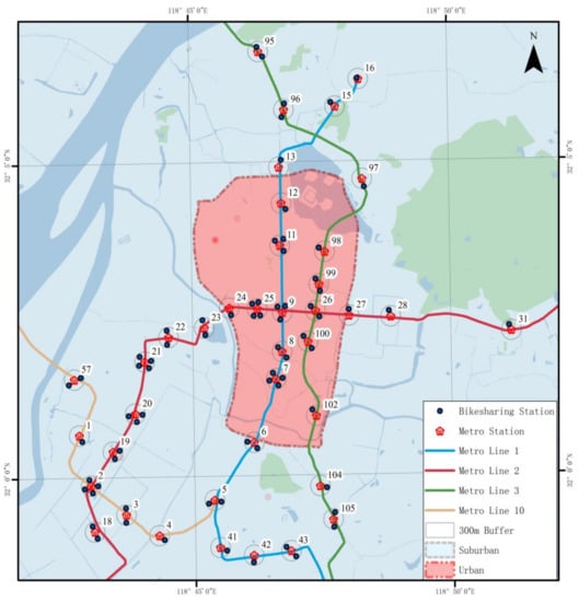
Figure 1.
Urban/suburban spatial distribution of 39 transfer pairs in the study area.
4.2. Explanatory Variables
The explanatory variables were selected based on the previous studies listed in Table 1. A total of 25 explanatory variables were chosen from three categories: demographics, travel and built environment. Specifically, the demographic variables included the proportions of males, local residents, and five age groups considering the sum of transfer trips at each metro station. The travel-related variables included travel distance on metro, travel distance on bikeshare, and ridership of metro and bikeshare.
Built environmental data were mainly provided by the Jiangsu Institute of Urban Planning and Design and the Jiangsu Institute of Urban Transport Planning. The built environmental variables included docks at bikeshare stations; density of bus stations, metro stations, and bikeshare stations; density of road networks; population density; job density; and numbers of types of point of interest (POI), including governmental, commercial/industrial, educational, entertainment, hospital, residential, and tourist attractions. All the variables associated with density were calculated within a service radius of 2 km of each metro station. The service radius of 2 km was estimated using recognized transfer data based on previous studies [20,33,34]. Additionally, all types of POI-related variables were counted within a service radius of 300 m of each terminal bikeshare station. The descriptive statistics and the unit of each potential independent variable are summarized in Table 6.
Table 6.
Descriptive statistics and units of explanatory variables.
5. Results and Analysis
5.1. Poisson Regression Model Result
To eliminate explanatory variables exhibiting multicollinearity, we used the Exploratory Regression tool in ArcGIS Pro to calculate the VIF indicators of each potential explanatory variable and to obtain the covariates of variables with VIF values greater than 10. The inspection results are shown in Table 7, which indicates that six variables had a VIF greater than 10: AGE2, AGE3, AGE4, AGE5, JD and PD. Based on the covariate column, four age variables were linearly correlated with each other, and JD and PD also presented a strong linear relationship. Thus, we excluded AGE3, AGE4, AGE2 and JD but retained AGE5 and PD, which had a smaller VIF relative to their covariates.
Table 7.
Variance inflation factor (VIF) and corresponding covariates of explanatory variables.
After solving the multicollinearity problem, we ran the global Poisson regression model using STATA to examine the relationship between the remaining variables and the dependent variable. In this paper, we set the significance level at P < 0.05 and assumed that variables with a P-value greater than 0.05 did not have a significant influence on the dependent variable and should be excluded from the Poisson regression model. We eliminated each insignificant variable using an iterative approach, and the final modeling results are shown in Table 8. A total of 17 variables were left after the down-selection. These variables were considered to significantly influence the transfer volume.
Table 8.
Poisson modeling results.
5.2. GWPR Model Results
Moran’s I test was conducted to determine whether some of these 17 variables were spatially autocorrelated and thus whether it is necessary to use the GWPR model for fitting these independent variables. Again, we used ArcGIS Pro to estimate the Moran’s I index of each selected explanatory variable after plotting the data on the geographical map with x-y coordinates. The estimation results are listed in Table 9. It can be seen that POLR, TDB, ROM, ROB, BUSD, BIKED, METROD and ENTERTAINMENT showed spatial autocorrelation with a significance level of P < 0.01, whereas the other explanatory variables did not show geographical variability.
Table 9.
Moran’s I test for each explanatory variable.
Therefore, a GWPR model was applied to explore the spatial heterogeneity of these variables with geographical variability. The modeling results are shown in Table 10. To further demonstrate the superiority and feasibility of the GWPR model, we compared it with the global Poisson regression model, which had the same explanatory variables as the GWPR model above. We calculated the AICc and AIC of the two models and found that the GWPR model had a significantly smaller AICc and AIC (shown in Table 11). This result indicates that GWPR better explained the data, suggesting that the GWPR model had a higher goodness-of-fit and better explanatory power.
Table 10.
Geographically weighted Poisson regression (GWPR) modeling results.
Table 11.
Comparison between GWPR and global Poisson regression modeling results.
5.3. Analysis and Discussion
As shown in Figure 2, Figure 3, Figure 4, Figure 5, Figure 6, Figure 7, Figure 8 and Figure 9, the effect of explanatory variables on metro-bikeshare transfer volume could be spatially investigated as in previous research [43,44,45]. The estimated coefficients of each paired metro-bikeshare station varied across regions, indicating that each selected variable was affected by local characteristics. Therefore, an analysis of the GWPR modeling performance can be used as a reference for government and bikeshare operators.
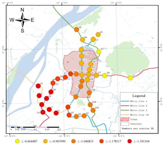
Figure 2.
Spatial distribution of estimated coefficients of proportion of local residents.
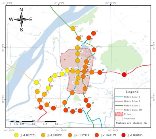
Figure 3.
Spatial distribution of estimated coefficients of the travel distance of bikeshare.
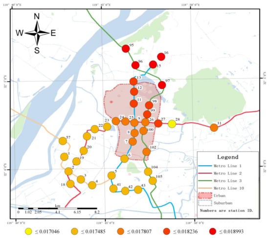
Figure 4.
Spatial distribution of estimated coefficients of ridership of metro.
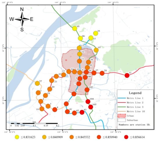
Figure 5.
Spatial distribution of estimated coefficients of ridership of bikeshare.
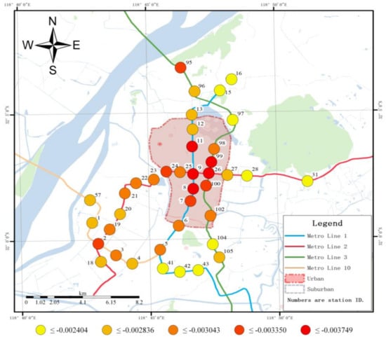
Figure 6.
Spatial distribution of estimated coefficients of the density of bus stations within a 2 km radius of a metro station.
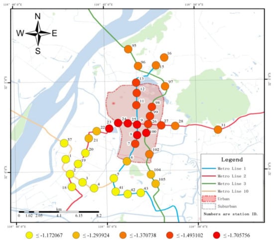
Figure 7.
Spatial distribution of estimated coefficients of the density of metro stations within a 2 km radius of a metro station.
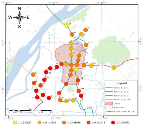
Figure 8.
Spatial distribution of estimated coefficients of the density of bikeshare stations within a 2 km radius of a metro station.
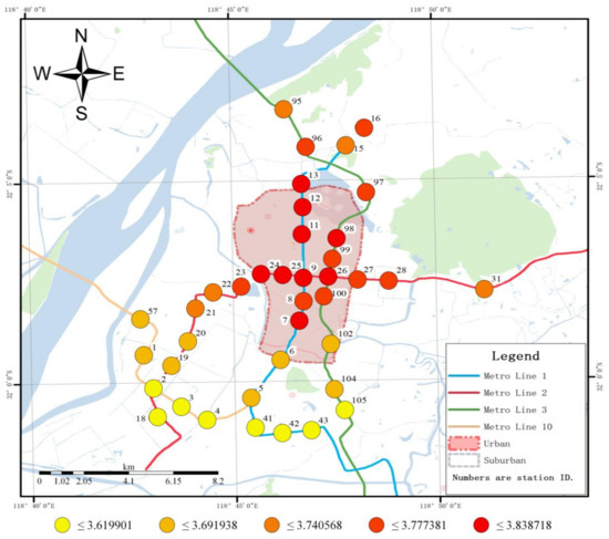
Figure 9.
Spatial distribution of estimated coefficients of the proportion of entertainment POI within 300 m radius of bikeshare stations.
As shown in Figure 2, there were clear negative correlations between proportion of local Residents (POLR) and metro-bikeshare transfer usage based on their coefficient values. As for the distribution of coefficients of POLR, the value was the lowest in the northwestern suburban area, where housing prices, which are US $5499 (34,369 RMB) per square meter, are higher than the average price of US $4800 (30,000) per square meter in Nanjing [58], indicating higher income and better life quality of local residents living in this area. As a result, these residents may use private vehicles for commuting, thus reducing the likelihood of using the metro-bikeshare transfer mode. The metro-bikeshare service should be enhanced, including suburban cycling infrastructure, among other metro-bikeshare services to greatly increase the metro-bikeshare usage by shifting local commuters away from using private vehicle travel modes.
A few European studies have shown that travel distance is a key factor that can explain the relationship between bike-and-ride, and faster public transportation tools (such as metro) tend to attract passengers from larger access and egress distances [22]. However, no research to date has examined how the travel distance on bikeshare affects metro-bikeshare integration in the context of Chinese cities. Our findings indicate that negative correlations exist between riding distance and metro-bikeshare transfer usage, which is quite understandable considering that people who use bikeshare for a longer distance are more likely to conduct the entire trip by bike and without needing to transfer to metro or any other modes for the remainder of their trip. As is show in Figure 3, the coefficient values were generally lower at the edge of the city, especially in underdeveloped areas. This phenomenon suggests that the combination of metro and bikeshare is still inadequate, and metro stations in those areas are sparsely distributed, so that people may have to take a bus, walk or use other transfer modes (but not metro) to finish their trips. Therefore, the government should provide more metro stations and support bikeshare stations within 2 km of metro stations in underdeveloped areas.
Figure 4 and Figure 5 show the spatial distribution of the coefficients for ridership of metro and bikeshare, respectively. It can be seen that positive correlations between ridership of metro and metro-bikeshare usage are primarily in the north of the city. Compared to the price in other areas in the suburbs, housing prices in northern regions, which are at US $4097 (25,608 RMB) per square meter, are relatively low [58]. Passengers living in this area use metro or metro-bikeshare to commute to urban areas as these two travel modes are more cost-effective [59,60]. In the south of the city, however, correlations between ridership of bikeshare and metro-bikeshare usage are much positive, compared with the least positive correlations in northern regions. A possible explanation is that when the first-stage bikeshare program of Nanjing was launched in the southern area in 2010, passengers there had accepted bikeshare as a feeder mode to metro [61]. Therefore, a scientific and reasonable dispatching approach needs to be implemented to solve the bikeshare imbalance problem in the northern and southern areas of the city. Additionally, an incentive policy to attract new users, such as a reduced price of any transfer between bikeshare and other public transit if a smart card is used, should be enacted.
Moreover, the density of bus, bikeshare, and other metro stations within a 2 km radius of a metro station had a great impact on the metro-bikeshare transfer volume. Specifically, bus and other metro stations nearby had a negative correlation with the transfer demand at one metro station. As for spatial patterns, the coefficients of bus and metro stations’ density show similar distributions in Figure 6 and Figure 7, reaching peaks in the core urban area. One factor that can explain this finding is the relatively well-developed public transport network, including more bus lines and a higher frequency of each line in urban areas, which makes bus another important feeder mode to metro in addition to bikeshare. When the density of bus stations increases, part of the transfer demand for metro-bikeshare will shift to metro-bus. Furthermore, the density of metro stations has a highly positive relationship with local development level. High density in urban areas often indicates heavy on-road traffic and, therefore, a higher risk of injury when riding bicycles. Thus, the higher the density, the more discouraged is the usage of bikeshare. In light of this, to improve metro-bikeshare service in urban areas, more bike lanes should be built, and illegal occupation of exclusive bicycle lanes by cars should be punished according to the law.
As Figure 8 shows, the density of bikeshare stations within a 2 km radius of a metro station is found to be positively correlated with metro-bikeshare usage. The coefficient reaches its highest value in the southern regions of suburban areas, which may indicate that the average riding distance in this area is currently quite unsatisfying, and the potential market for metro-bikeshare transfer is great. As a result, more bikeshare stations should be built in suburban areas to shorten the average riding distance and potentially attract more people to apply bikeshare as a feeder mode to metro, consistent with the results of Parkin et al. [62] and Faghih-Imani A et al. [63].
As shown in Figure 9, the coefficient of entertainment POI was highest in the urban area, especially around Station 9 (XinJieKou metro station), where most of the major shopping centers are located. This result indicates that more recreational area is expected to bring more metro-bikeshare transfers. This finding is intuitive because the traffic conditions around the entertainment POI are congested, especially during peak transit hours. The relatively higher density of bikeshare stations in urban areas improves the accessibility of bikeshare. Passengers who prefer cheaper and time-saving travel modes are more likely to choose bikeshare to reach entertainment destinations. On the other hand, the roads in suburban areas are mainly built for the sake of motorized vehicles, and metro stations in suburban areas fail to serve many large-scale entertainment sites, so that people must arrive there by car or taxi. Few people are willing to choose the bikeshare-metro travel mode for entertainment in suburban districts, principally due to the low density of metro stations. Therefore, it is suggested that the government should increase metro stations in suburban districts to improve the accessibility of some entertainment places, which will in turn attract more people to choose the metro-bikeshare travel mode.
6. Conclusions
This paper explores the bikeshare mode as a feeder to metro by mining smart-card data. First, we propose a novel data-fusion method to isolate valid metro-bikeshare transfer trips by matching the metro and bikeshare smart cards of one passenger. Three recognition rules are generated: the maximum time for transfer is 10 min, the maximum transfer distance is 300 m, and at least 30 transfer trips occurred at the paired transfer stations over three consecutive weeks. To better understand the key factors associated with metro-bikeshare usage, this study respectively applies a global Poisson regression model and GPWR model to identify the key factors to the metro-bikeshare usage of a total of 39 paired metro-bikeshare stations in Nanjing. In terms of AICc, AIC and Moran’s I testing, the GPWR model performs better than the global Poisson regression model. According to the estimation results of the GWPR model, eight estimated coefficients have been visualized across regions. Specifically, POLR, TDB, BUSD and METROD have a negative effect on metro-bikeshare usage, while ROM, ROB, BIKED and ENTERTAINMENT have a positive effect. Based on these findings, strategies that promote metro-bikeshare integration are then proposed.
The current work can be extended by obtaining additional data. Because we obtained March 2016 data from only the Nanjing Bikeshare System and the Nanjing Metro System, we could only analyze the influential factors of metro-bikeshare integration in this city during that month. Obtaining smart-card data from other cities would allow us to examine whether the factors influencing transfer in other cities are consistent with those in Nanjing. Moreover, smart-card data covering a longer time period should be obtained to examine whether transfer behavior varies seasonally. Additionally, we could further establish other spatial regression models (e.g., SEM and SLM) in addition to the GWPR model and compare their performance. Despite this, the most suitable spatial model can be selected, and its application conditions can be summarized in similar research.
Author Contributions
Y.J. and X.M. conceived of and designed the experiments, M.Y. and Y.J. performed the experiments, L.G. drew and analyzed the maps, and X.M. wrote the paper.
Funding
This research was funded by [the International Cooperation and Exchange of the National Natural Science Foundation of China] grant number [51561135003], [the Key Project of National Natural Science Foundation of China] grant number [51338003], [the Natural Science Foundation of Zhejiang Province, China] grant number [LY17E080013] and [Natural Science Foundation of Ningbo City, China] grant number [2016A610112].
Acknowledgments
We are grateful for the comments and suggestions from the editor and four anonymous reviewers who helped improve the paper.
Conflicts of Interest
The authors declare no conflict of interest.
References
- Qiu, L.-Y.; He, L.-Y. Bike Sharing and the Economy, the Environment, and Health-Related Externalities. Sustainability 2018, 10, 1145. [Google Scholar] [CrossRef]
- Ma, T.; Liu, C.; Erdoğan, S. Bicycle Sharing and Public Transit: Does Capital Bikeshare Affect Metrorail Ridership in Washington, D.C.? Transp. Res. Rec. 2015, 2534, 1–9. [Google Scholar] [CrossRef]
- Maizlish, N.; Woodcock, J.; Co, S.; Ostro, B.; Fanai, A.; Fairley, D. Health cobenefits and transportation-related reductions in greenhouse gas emissions in the San Francisco Bay Area. Am. J. Public Health 2013, 103, 703–709. [Google Scholar] [CrossRef] [PubMed]
- Yang, M.; Liu, X.; Wang, W.; Li, Z.; Zhao, J. Empirical Analysis of a Mode Shift to Using Public Bicycles to Access the Suburban Metro: Survey of Nanjing, China. J. Urban Plan. Dev. 2015, 142, 05015011. [Google Scholar] [CrossRef]
- Fishman, E.; Washington, S.; Haworth, N. Bike share’s impact on car use: Evidence from the United States, Great Britain, and Australia. Transp. Res. Part D 2014, 31, 13–20. [Google Scholar] [CrossRef]
- Pucher, J.; Buehler, R. Cycling towards a more sustainable transport future. Transp. Rev. 2017, 37, 689–694. [Google Scholar] [CrossRef]
- Yahya, B. Overall Bike Effectiveness as a Sustainability Metric for Bike Sharing Systems. Sustainability 2017, 9, 2070. [Google Scholar] [CrossRef]
- Shaheen, S.A. Hangzhou Public Bicycle: Understanding Early Adoption and Behavioral Response to Bikesharing in Hangzhou, China. Transp. Res. Board 2013, 2247, 34–41. [Google Scholar] [CrossRef]
- Ji, Y.; Fan, Y.; Ermagun, A.; Cao, X.; Wang, W.; Das, K. Public bicycle as a feeder mode to rail transit in China: The role of gender, age, income, trip purpose, and bicycle theft experience. Int. J. Sustain. Transp. 2017, 11, 308–317. [Google Scholar] [CrossRef]
- Midgley, P. Bicycle-Sharing Schemes: Enhancing Sustainable Mobility in Urban Areas. Commun. Sustain. Dev. 2011, 19, 1–12. [Google Scholar]
- Zhao, P.; Li, S. Bicycle-metro integration in a growing city: The determinants of cycling as a transfer mode in metro station areas in Beijing. Transp. Res. Part A 2017, 99, 46–60. [Google Scholar] [CrossRef]
- Bike-Sharing World Map. 2017. Available online: bikesharingmap.com (accessed on 2 July 2017).
- Shaheen, S.; Martin, E.; Cohen, A. Public Bikesharing and Modal Shift Behavior: A Comparative Study of Early Bikesharing Systems in North America. Int. J. Transp. 2013, 1, 35–54. [Google Scholar] [CrossRef]
- Tang, Y.; Pan, H.; Shen, Q. Bike-Sharing Systems in Beijing, Shanghai and Hangzhou and Their Impact on Travel Behaviour; Department of Urban Planning, Tongji University: Shanghai, China, 2010. [Google Scholar]
- Fishman, E. Bikeshare: A Review of Recent Literature. Transp. Rev. 2015, 1647, 1–22. [Google Scholar] [CrossRef]
- Lan, J.; Ma, Y.; Zhu, D.; Mangalagiu, D.; Thornton, T.F. Enabling Value Co-Creation in the Sharing Economy: The Case of Mobike. Sustainability 2017, 9, 1504. [Google Scholar] [CrossRef]
- Shaheen, S.A.; Guzman, S.; Zhang, H. Bikesharing across the Globe. In City Cycling; The MIT Press: Cambridge, MA, USA, 2012; pp. 183–210. [Google Scholar]
- Yang, H.; Lu, X.; Cherry, C.; Liu, X.; Li, Y. Spatial variations in active mode trip volume at intersections: A local analysis utilizing geographically weighted regression. J. Transp. Geogr. 2017, 64, 184–194. [Google Scholar] [CrossRef]
- Bachand-Marleau, J.; Larsen, J.; El-Geneidy, A. Much-anticipated marriage of cycling and transit: How will it work? Transp. Res. Rec. 2011, 2247, 109–117. [Google Scholar] [CrossRef]
- Lee, J.; Choi, K.; Leem, Y. Bicycle-Based transit-oriented development as an Alternative to Overcome the Criticisms of the Conventional transit-oriented development. Int. J. Sustain. Transp. 2016, 10, 975–984. [Google Scholar] [CrossRef]
- Du, M.; Cheng, L. Better Understanding the Characteristics and Influential Factors of Different Travel Patterns in Free-Floating Bike Sharing: Evidence from Nanjing, China. Sustainability 2018, 10, 1244. [Google Scholar] [CrossRef]
- Martens, K. The bicycle as a feedering mode: Experiences from three European countries. Transp. Res. Part D 2004, 9, 281–294. [Google Scholar] [CrossRef]
- Yang, R.; Long, R. Analysis of the Influencing Factors of the Public Willingness to Participate in Public Bicycle Projects and Intervention Strategies—A Case Study of Jiangsu Province, China. Sustainability 2016, 8, 349. [Google Scholar] [CrossRef]
- Martens, K. Promoting bike-and-ride: The Dutch experience. Transp. Res. Part A 2007, 41, 326–338. [Google Scholar] [CrossRef]
- Pan, H.; Shen, Q.; Xue, S. Intermodal Transfer between Bicycles and Rail Transit in Shanghai, China. Transp. Res. Rec. 2010, 2144, 181–188. [Google Scholar] [CrossRef]
- Fan, Y.; Guthrie, A.; Levinson, D. Waiting time perceptions at transit stops and stations: Effects of basic amenities, gender, and security. Transp. Res. Part A 2016, 88, 251–264. [Google Scholar] [CrossRef]
- Cheng, Y.H.; Liu, K.C. Evaluating bicycle-transit users’ perceptions of intermodal inconvenience. Transp. Res. Part A 2012, 46, 1690–1706. [Google Scholar] [CrossRef]
- Li, Z.-C.; Yao, M.-Z.; Lam, W.H.K.; Sumalee, A.; Choi, K. Modeling the Effects of Public Bicycle Schemes in a Congested Multi-Modal Road Network. Int. J. Sustain. Transp. 2014, 9, 282–297. [Google Scholar] [CrossRef]
- Yang, M.; Zacharias, J. Potential for Revival of the Bicycle in Beijing. Int. J. Sustain. Transp. 2015, 10, 517–527. [Google Scholar] [CrossRef]
- Arbis, D.; Rashidi, T.H.; Dixit, V.V.; Vandebona, U. Analysis and Planning of Bicycle Parking for Public Transport Stations. Int. J. Sustain. Transp. 2016, 10, 495–504. [Google Scholar] [CrossRef]
- Chen, C.F.; Cheng, W.C. Sustainability SI: Exploring Heterogeneity in Cycle Tourists’ Preferences for an Integrated Bike-Rail Transport Service. Netw. Spat. Econ. 2016, 16, 83–97. [Google Scholar] [CrossRef]
- Griffin, G.P.; Sener, I.N. Planning for Bike Share Connectivity to Rail Transit. J. Public Transp. 2016, 19, 1–22. [Google Scholar] [CrossRef] [PubMed]
- Hochmair, H.H. Assessment of Bicycle Service Areas around Transit Stations. Int. J. Sustain. Transp. 2014, 9, 15–29. [Google Scholar] [CrossRef]
- Iacono, M.; Krizek, K.J.; El-Geneidy, A. Measuring non-motorized accessibility: Issues, alternatives, and execution. J. Transp. Geogr. 2010, 18, 133–140. [Google Scholar] [CrossRef]
- Mohanty, S.; Bansal, S.; Bairwa, K. Effect of integration of bicyclists and pedestrians with transit in New Delhi. Transp. Policy 2017, 57, 31–40. [Google Scholar] [CrossRef]
- Sun, Y.; Mobasheri, A.; Hu, X.; Wang, W. Investigating Impacts of Environmental Factors on the Cycling Behavior of Bicycle-Sharing Users. Sustainability 2017, 9, 1060. [Google Scholar] [CrossRef]
- Saghapour, T.; Moridpour, S.; Thompson, R.G. Measuring cycling accessibility in metropolitan areas. Int. J. Sustain. Transp. 2017, 11, 381–394. [Google Scholar] [CrossRef]
- Chen, L.; Pel, A.J.; Chen, X.; Sparing, D.; Hansen, I.A. Determinants of Bicycle Transfer Demand at Metro Stations: An Analysis of Stations in Nanjing, China. Transp. Res. Rec. 2012, 2276, 131–137. [Google Scholar] [CrossRef]
- Mohanty, S.; Blanchard, D.S. Complete Transit: Evaluating Walking and Biking to Transit Using a Mixed Logit Mode Choice Model. In Proceedings of the 95th Annual Meeting of the Transportation Research Board, Washington, DC, USA, 10–14 January 2016; p. 21. [Google Scholar]
- Puello, L.L.P.; Geurs, K. Modelling observed and unobserved factors in cycling to railway stations: Application to transit-oriented-developments in the Netherlands. Eur. J. Transp. Infrastruct. Res. 2015, 15, 27–50. [Google Scholar]
- Martin, E.W.; Shaheen, S.A. Evaluating public transit modal shift dynamics in response to bikesharing: A tale of two U.S. cities. J. Transp. Geogr. 2014, 41, 315–324. [Google Scholar] [CrossRef]
- Faghih-Imani, A.; Eluru, N. Examining the impact of sample size in the analysis of bicycle-sharing systems. Transp. A Transp. Sci. 2017, 13, 139–161. [Google Scholar] [CrossRef]
- Chiou, Y.C.; Jou, R.C.; Yang, C.H. Factors affecting public transportation usage rate: Geographically weighted regression. Transp. Res. Part A 2015, 78, 161–177. [Google Scholar] [CrossRef]
- Bao, J.; Liu, P.; Yu, H.; Xu, C. Incorporating twitter-based human activity information in spatial analysis of crashes in urban areas. Accid. Anal. Prev. 2017, 106, 358–369. [Google Scholar] [CrossRef] [PubMed]
- Qian, X.; Ukkusuri, S.V. Spatial variation of the urban taxi ridership using GPS data. Appl. Geogr. 2015, 59, 31–42. [Google Scholar] [CrossRef]
- Yang, W.; Chen, B.Y.; Cao, X.; Li, T.; Li, P. The spatial characteristics and influencing factors of modal accessibility gaps: A case study for Guangzhou, China. J. Transp. Geogr. 2017, 60, 21–32. [Google Scholar] [CrossRef]
- Vandenbulcke, G.; Dujardin, C.; Thomas, I.; de Geus, B.; Degraeuwe, B.; Meeusen, R.; Panis, L.I. Cycle commuting in Belgium: Spatial determinants and “re-cycling” strategies. Transp. Res. Part A 2011, 45, 118–137. [Google Scholar] [CrossRef]
- Wang, C.H.; Chen, N. A geographically weighted regression approach to investigating the spatially varied built-environment effects on community opportunity. J. Transp. Geogr. 2017, 62, 136–147. [Google Scholar] [CrossRef]
- Kerkman, K.; Martens, K.; Meurs, H. A multilevel spatial interaction model of transit flows incorporating spatial and network autocorrelation. J. Transp. Geogr. 2017, 60, 155–166. [Google Scholar] [CrossRef]
- Wang, Y.; Feng, S.; Deng, Z.; Cheng, S. Transit premium and rent segmentation: A spatial quantile hedonic analysis of Shanghai Metro. Transp. Policy 2016, 51, 61–69. [Google Scholar] [CrossRef]
- Liu, X.; Roberts, M.C.; Sioshansi, R. Spatial effects on hybrid electric vehicle adoption. Transp. Res. Part D 2017, 52, 85–97. [Google Scholar] [CrossRef]
- Akar, G.; Chen, N.; Gordon, S.I. Influence of neighborhood types on trip distances: Spatial error models for Central Ohio. Int. J. Sustain. Transp. 2016, 10, 284–293. [Google Scholar] [CrossRef]
- Kutner, M.H.; Nachtsheim, C.; Neter, J. Applied Linear Regression Models, 4th ed.; McGraw-Hill/Irwin Education: New York, NY, USA, 2005. [Google Scholar]
- Alexander, N. Bayesian Disease Mapping: Hierarchical Modeling in Spatial Epidemiology. J. R. Stat. Soc. 2011, 174, 512–513. [Google Scholar] [CrossRef]
- Fotheringham, A.S.; Charlton, M.E.; Brunsdon, C. Geographically Weighted Regression: A Natural Evolution of the Expansion Method for Spatial Data Analysis. Environ. Plan. A 1998, 30, 1905–1927. [Google Scholar] [CrossRef]
- Faghihimani, A.; Eluru, N. Analysing Destination Choice Preferences in Bicycle Sharing Systems: An Investigation of Chicago’s Divvy System. In Proceedings of the 94th Annual Meeting on Compendium of Transportation Research Board, Washington, DC, USA, 11–15 January 2015. [Google Scholar]
- Nanjing Urban Planning Bureau. Planning Standards for Public Facilities; Nanjing Urban Planning Bureau: Nanjing, China, 2015.
- LianJia Housing Price Report. Available online: https://nj.lianjia.com/fangjia/ (accessed on 25 April 2018).
- Pucher, J.; Buehler, R. Integrating Bicycling and Public Transport in North America. J. Public Transp. 2009, 12, 79–104. [Google Scholar] [CrossRef]
- Brons, M.; Givoni, M.; Rietveld, P. Access to railway stations and its potential in increasing rail use. Transp. Res. Part A 2009, 43, 136–149. [Google Scholar] [CrossRef]
- Zhao, J.; Wang, J.; Deng, W. Exploring bikesharing travel time and trip chain by gender and day of the week. Transp. Res. Part C 2015, 58, 251–264. [Google Scholar] [CrossRef]
- El-Assi, W.; Mahmoud, M.S.; Habib, K.N. Effects of built environment and weather on bike sharing demand: A station level analysis of commercial bike sharing in Toronto. Transportation 2017, 44, 589–613. [Google Scholar] [CrossRef]
- Faghih-Imani, A.; Eluru, N.; El-Geneidy, A.M.; Rabbat, M.; Haq, U. How land-use and urban form impact bicycle flows: Evidence from the bicycle-sharing system (BIXI) in Montreal. J. Transp. Geogr. 2014, 41, 306–314. [Google Scholar] [CrossRef]
© 2018 by the authors. Licensee MDPI, Basel, Switzerland. This article is an open access article distributed under the terms and conditions of the Creative Commons Attribution (CC BY) license (http://creativecommons.org/licenses/by/4.0/).