Efficiency of the Public Pensions Funds on the Socially Responsible Equities of Mexico

Abstract

In the present work, we test the mean-variance efficiency that Mexican public pension funds would have shown had these invested their local equity portfolio component only in socially responsible stocks. With a daily simulation (from 1 January 2005 to 31 July 2018) of the Standard & Poors (S&P) Mexico target risk indices, we found that there was no significant difference between the more conservative pension funds that invested only in the Price Index and Quotations (IPC) sustainable index against the ones that invested in the conventional IPC. In the case of the more aggressive type of pension funds (those with a higher Mexican equity investment level), a lower mean-variance efficiency would have been observed had these invested in the IPC sustainable index. We also found, with a two-regime Markov-switching analysis, that socially responsible investment would have been better for most of these pension funds during distress time periods. Even if our results do not give strong short-term proof for the use of a socially responsible investment strategy in the most aggressive pension funds, we found that the benefits will be observed in the long-term, due to a better performance during distress time periods and the lag effect of mid and small-cap stocks in the performance.

1. Introduction

The Mexican public pension fund system is one of the key subjects for sustainable long-term macroeconomic growth in Mexico due to the fact that its proper funding ensures consumption levels in the future. This system, with an origin in 1917 in Article 123 of the Mexican Republic’s Political Constitution, allowed the creation of the Mexican Institute of Social Security (IMSS) and its corresponding law. With this law, the Mexican public pension system started, with funding from the government, the workers, and the patrons, and it was focused on all public and private companies and their workers.

At the beginning, this pension system had a defined-benefit pension funding scheme, but in 1997, given the recommendations of the International Monetary Fund and potential future Public budget risks, Mexico reformed this system into one of defined-contribution in which all the pension savings are saved in an individual account known as SIEFOREs (the acronym in Spanish of Sociedad de Inversión Especialidada en Fondos para el Retiro or Retirement Mutual Fund). These SIEFOREs, as a sort of mutual fund, are managed by a company known as AFORE (Administradora de FOndos para el REtiro or Pension Mutual Fund Manager) and the selection or change to a given SIEFORE is made by each pension saver once a year.

Since their inception in 1997, the SIEFOREs were allowed to invest only in Mexican government and Mexican corporate debt, but in January 2005, they were allowed to invest part of their proceedings in Mexican stocks. With this change, the SIEFOREs were split into two types: Type 1 (henceforth SB1) SIEFORE for pension savers close to retirement and type 2 (SB2) for younger savers that were allowed to invest in Mexican equity. Later, in March of 2008, the type 2 SIEFOREs were split into four types, allowing five types of SIEFOREs in all the pension savings system. This change was made in order to have a life-cycle investment policy [1]. Since then, the SIEFORES have been allowed to invest not only in Mexican debt and equity, but also in international debt, international stocks, real estate, and commodities. Finally, in February of 2013, the CONSAR (National Pension Savings System Comission) changed the life-cycle investment scheme and merged type 4 and type 5 SIEFOREs into one.

With this public and official investment policy, the SIEFOREs manage the resources of pension savers according to their age. The type 4 SIEFORE (henceforth SB4) is the riskiest type of SIEFORE and is for pension savers of 36 years or less of age. Type 3 (SB3) has an investment policy for people between 37 and 45 years, the type 2 or SB2 is for savers between 46 and 59 years old, and, finally, SB1 or type 1 SIEFORE is the most conservative and is planned for savers between 60 and 65 years. There is a special type of SIEFORE, the basic retirement pension type (SB0), that is for people of 60 years or more with a pension. Due to the fact that these types of SIEFORE do not allow investment in equities and are for retired people, we will omit the study of these herein.

For further reference, in

Table 1. Investment policy allowed by CONSAR (maximum investment levels per type of security).

Type of Security Allowed or Portfolio Parameter	SB0	SB1	SB2	SB3	SB4
Value at Risk	0.70%	0.70%	1.10%	1.40%	2.10%
Debt issued or endorsed by the Mexican government in MXN (with mxBB to mxAAA S&P credit rate)	100.00%	100.00%	100.00%	100.00%	100.00%
Foreign securities (BBB- to AAA credit rate for debt)	0.00%	20.00%	20.00%	20.00%	20.00%
Equity	0.00%	10.00%	30.00%	35.00%	45.00%
Foreign currency	0.00%	30.00%	30.00%	30.00%	30.00%
Securitizations	0.00%	10.00%	15.00%	20.00%	30.00%
Structured securities	0.00%	10.00%	15.00%	20.00%	20.00%
Mexican REITs (FIBRAs) and foreign REITs	0.00%	5.00%	10.00%	10.00%	10.00%
Inflation protected securities (minimum investment allowed and 100% as upper investment limit)	0.00%	51.00%	0.00%	0.00%	0.00%
Commodities	0.00%	0.00%	5.00%	10.00%	10.00%

Source: Own elaboration departing from the investment policy of CONSAR [2].

, we summarize the key features of the official investment policy allowed by CONSAR [2] for each type of SIEFORE.

Several studies have been carried out about the appropriateness and macroeconomic benefits of this pension system reform made in 1997 and about the benefits of its investment performance, but until now, few reviews exist that seize the impact of socially responsible investment (henceforth SRI) in the investment policy and performance of pension funds. This issue is of interest because SRI, even though it is not new, has evolved since the decade of the 1970s to perform activism against companies that are not considering the social welfare, ethical orientation, or environmental impact of their activities. This type of investment has evolved as an investment style since the 1970s and several public well-known pension funds, such as the California Public Employees’ Retirement System (CALPERS) or the Swedish National Pension Funds (among two well-known examples), have focused their investment policy in only SRI companies (and their issued securities). Another motivation for the use of SRI in the investment industry (especially among mutual funds) is the implementation of tax incentives to favor SRI and socially responsible lending [3,4].

Until now, there has only been one study [5] that has measured the benefit of SRI in the Mexican SIEFOREs, but this test was made in a theoretical minimum variance and in a Max Sharpe portfolio, given the investment policy of Table 1. In this review, the authors test an investment policy with Mexican and international debt and stocks along with commodities, but their performance is not referenced or linked to the performance of a well-known, public and testable performance benchmark of the SIEFORES, a benchmark that does not exist nowadays in Mexico.

As a first partial solution of a testable and public SIEFORE benchmark, Standard & Poors Dow Jones (henceforth S&P) started to measure the performance of the four types of SIEFORES (SB1 to SB4) with the publication of the S&P/BMV Mexico Target Risk index series [6]. These indexes are four public benchmarks that measure the performance of each type of SIEFORE given the investment levels shown in

Table 2. The investment policy of the four S&P/BMV Mexico target risk indices (investment levels in each type of security).

Index Used in This Paper	Type of Asset or Security	Conservative	Moderate	Growth	Aggressive
S&P/BMV Sovereign CETES	Cash	10.00%	3.00%	3.00%	3.00%
S&P/BMVMEX Government Bonos M 1–5 year	Fixed rate Sovereign fixed income	9.60%	7.60%	6.80%	---
S&P/BMVMEX Government Bonos M 5–10 year	Fixed rate Sovereign fixed income	6.40%	22.80%	6.80%	6.00%
S&P/BMVMEX Government Bonos M 10–20 year	Fixed rate Sovereign fixed income	---	7.60%	20.40%	6.00%
S&P/BMVMEX Government Bonos M 20+ year	Fixed rate Sovereign fixed income	---	---	---	18.00%
S&P/BMVMEX Government Udibonos 1–5 year	Inflation-linked Sovereign fixed income	33.00%	5.30%	---	---
S&P/BMVMEX Government Udibonos 5–10 year	Inflation-linked Sovereign fixed income	22.00%	15.90%	5.10%	---
S&P/BMVMEX Government Udibonos 10–20 year	Inflation-linked Sovereign fixed income	---	5.30%	5.10%	4.40%
S&P/BMVMEX Government Udibonos 20+ year	Inflation-linked Sovereign fixed income	---	---	15.30%	4.40%
S&P/BMVMEX CORPOTRAC	Corporate bonds	15.00%	12.50%	12.50%	10.00%
S&P Global 1200	International equity	3.00%	12.00%	15.00%	15.00%
S&P/BMV IPC or S&P/BMV IPC Sustainable	Local equity	1.00%	8.00%	10.00%	20.00%

Source: Own elaboration based on S&P Dow Jones indices LLC [6].

, and they are assumed to be a good proxy of the investment policy given by CONSAR [2]. This last assumption will not be tested here, given the perspective of the present work. Departing from this issue and contrary to De la Torre and Macias [5], who use their own theoretical portfolios, we will use the investment policy of the aforementioned target risk indexes to simulate the impact of SRI in the investment policy of the four types of SIEFOREs (SB1, SB2, SB3, and SB4).

For this purpose, we will simulate (recalculate) the performance of each target risk index with either the conventional S&P/BMV IPC index (our control or reference pension portfolio) or the S&P/BMV IPC sustainable one (our experimental pension portfolio) in their holdings.

We made this test by the fact that the IPC index (henceforth IPC) is the main equity benchmark in Mexico and is integrated by the stocks of the 35 biggest and most traded companies in the Mexican Stock Exchange. As a consequence, it contains stocks of socially responsible companies that are members of the IPC sustainable (henceforth IPCS) and companies that are not members of it. With this in mind, we tested the mean-variance efficiency that a given Mexican public pension fund or SIEFORE would have had, had it invested in only SRI stocks (in the IPCS), compared with the observed one of a SIEFORE that invested in the conventional one or IPC.

Our rationale is that, if we find evidence in favor of investing in Mexican SRI stocks only, we can make a policy recommendation to CONSAR to promote socially responsible investing among SIEFOREs and also to promote, among other institutional investors, an SRI only perspective in their investment policy.

Following this rationale and research motivations, in the next section, we will briefly review the most relevant research related to SRI and the impact of SRI in pension funds, followed by a section with quantitative tests and a review of the simulated results. In the concluding section, we will mention our main findings and conclusions, along with the suggestions for further research.

2. Literature Review

2.1. ESG, Stakeholders Theory, and Socially Responsible Investment

Before we start with the literature review that motivates this paper, it is important to mention what will be understood as socially responsible investment, social responsibility, or sustainability and how will these terms will be used herein. We also will briefly discuss the history of the S&P/BMV IPC sustainable index that is the SRI benchmark of interest.

As a starting point, it is important to mention that we are not going to involve in the discussion of the term sustainable in comparison with the one of socially responsibility. We do this by the fact that this kind of discussion is proper of a management space in which it is of interest to determine what it is understood as corporate social responsibility (CSR). Also, in this kind of academic space, it is more proper to discuss what is understood as CSR in comparison with the term, sustainability, including the discussion of whether these are proxy or different terms in their conception and application. Even if it is a closely related discussion to the purposes followed herein, we want to point out that the quality of being socially responsible is a qualitative process that leads to a screening process in which an investor decides what are the type of companies in which she will invest her proceedings. From a historical perspective, socially responsible investment has its ancient origins in religious texts, such as the Tora, the Bible, or the Coran. Also, some Hinduist and Buddhist precepts have been considered to decide in which economic activities are more appropriate to invest in. Departing from those moral and religious practices, there are some documented records [7,8,9] that suggest that the Puritans or the Muslim people have a specific screening process to determine what type of activities to invest in or to finance [7,10,11]. In the decade of the 1970’s, SRI started in the United States as a form of activist investing in order to make a negative screening process of the stocks of companies involved in weapon production or supplies for the U.S. war in Vietnam [7]. Later, it evolved to penalize against companies with either high environmental impact in their activities or related to negative social situations, such as the apartheid in South Africa [7].

Since then, socially responsible investment has evolved in a parallel, but different fashion to the concepts of sustainability declared in the United Nations (U.N.) Millennium declaration [12] or its 60/1 resolution [13], in which the concept of sustainability in business and economic activity is integrated in three pillars: the environmental, the social, and the government (ESG). In the first one, it is well known that the company or institution must take the environmental impact that its activities have, along with the social benefit (social pillar) that these must have with its customers, its suppliers, its competitors, and the social group in which they trade. The last pillar is one of interest (especially since the 2001 corporate scandals) because it relates the level of disclosure and agency risk reduction that a company must have with its shareholder, competitors, or authorities.

In a parallel fashion to ESG, and being one of the most observable theories in the field, the stakeholder theory of Friedman [14] promotes that the company must pay more attention to the relationship and creation of value not only to its stockholders (as external stakeholder), but also to other internal and external stakeholders, such as the employees, owners, and managers or the customers, suppliers, society, government, creditors, or shareholders, respectively.

This historical development of ESG and stakeholder theory leads to two very specific, but closely related theories in organizational management that have their implication in economics and finance, due to the impact that the proper management of a company or a group of these have in a society.

Departing from this and by following Eccles and Viviers’ [15] conclusions, we observe that these previous ESG and stakeholder theories are related, given their purpose of determining the long-term performance (financial, social, corporate government, and economic) of a given company.

From the aforementioned activist investment and also the evolution of ESG, it is of interest for us to mention that the concepts of “sustainable investment”, “socially responsible investment”, “ethical investment”, and related will be understood as synonymous terms for the purposes followed herein. As Berry and Junkus [16] observe, these types of investing activities have different screening processes that are either positive (including stocks that have a certain ESG score or quality) or negative (excluding stocks of companies that have negative social or environmental impact activities). Also, these screening processes are different and what is ethical for one investor could not be as such for another one. With this in mind and for the purposes of this review, it is of interest to note that the sustainable or socially responsible investment will be reduced to an asset-allocation practice or style in which the investor decides which metrics to use in order to screen and select the securities that she will hold in her portfolio. This last action will have an impact in her performance and mean-variance efficiency that we want to test in this paper in Mexican Public pension funds.

After this brief discussion, we will use the terms, socially responsible investment or sustainable investment, indistinctly and we will use the ESG scores supplied by EIRIS and Standard & Poors (S&P) to determine which stocks must be a member of the S&P/BMV IPC sustainable (IPCS).

This last index is the first socially responsible or sustainability index in Mexico and was originally developed by the Mexican Stock Exchange (MSE) in order to select the 35 most ESG companies from the universe of the S&P/BMV IPC Comp (IPCcomp) index. This last benchmark is a small, mid, and large-cap index conformed of the 60 biggest and most tradable stocks in the MSE. With the support of EIRIS and the Anahuac university, the MSE started to score its issuing companies and to make the selection of the 35 IPCS until 14 May 2015, when S&P reached an index licensing and distribution agreement with the MSE and now is S&P, who makes most of the ESG scoring, calculation, and distribution of this index.

The other index of interest, the S&P/BMV IPC (IPC), is one of the oldest, most known, and most used market benchmarks by investors in Mexico and abroad. Since its inception in 30 October 1978 [17], the index has been a 35 blue-chip stocks (the biggest and most traded stocks) and has measured the performance of the most important companies in the MSE. Contrary to the IPCcomp and the IPCS, the IPC is a large-cap only index, given its methodology and can have, as members, stocks of either highly ESG scored companies or even no ESG ones. This make the IPC and the IPCcomp, in terms of ESG, “conventional” style indexes by the fact that these indexes include either ESG or no-ESG stocks. Departing from this, we will use the term, “conventional investing”, to refer to the IPC index that includes ESG and no-ESG stocks and the term, “sustainable investment”, “ESG investment”, or “socially responsible investment (SRI)”, to refer to the style of interest in the IPCS.

With this in mind, we will simulate the performance that the four type of SIEFORES would have had in their investment policy had they invested only in ESG stocks (only in the IPCS) against the result attained with the investment made nowadays with the IPC index as one of the main “conventional investment” benchmarks. Before we present the parameters of this simulation and the observed results, we will make a brief discussion of the previous research made in sustainable investment and its application in pension funds.

2.2. Literature Review of the Works that Motivate this Paper

Even if the benefits of SRI have been tested in the pioneering works of Hamilton, Jo, and Statman [18] and Statman [19], the development of the literature that motivates the current work is wide in extension and conclusions. Some previous works have studied the performance of SRI mutual funds against conventional ones [3,20,21,22,23] as we do herein. These works have conclusions in favor and against SRI and most of them test the performance of either SRI mutual funds or indexes. Their conclusions give strong support to SRI activities. In order to investigate the causes of these results in SRI mutual funds, Przychodzen et al. [23] applied a questionnaire among U.S., Canadian, U.K, Polish, and Spanish mutual funds and they found that the SRI activities are highly motivated by a herding behavior and to sort of short-term risk reduction, a result that motivates the present paper by the fact that we want to simulate the investment policy of the three type of SIEFOREs with the S&P target-risk methodology. We do this in order to determine the potential risk reduction benefits of an only SRI local equity strategy.

By applying multifactor models, such as Carhart’s [24], these studies found no evidence in favor or against SRI in terms of alpha generation or performance. In another perspective, Humphrey and Tan [22] gave proof against Hong and Kacpersyk’s [25] conclusions that the sinful stocks (the ones that have a high social, environmental, or economic impact in their activities) have a better performance than the SRI stocks by the fact that the previous are neglected and mispriced. They gave proof against the aforementioned sinful position in stocks of the S&P500 with KLD SRI scores and also gave proof of the positive validity of the shunned-stock hypothesis previously suggested and tested by Derwal, Koedjik, and Horst [26]. This hypothesis stated that SRI could lead to lower financial return than either conventional or the sinful investment strategy by the fact that the increased demand of SRI stocks (due to a potential herding behavior as Przychodzen et. al. [23] found out) increases their price and lowers the returns paid. This issue, as we will mention in our results and conclusions, will have a short-term impact in the performance of the most aggressive type of public pension funds in Mexico.

From another perspective and to set aside the noise produced by fund management factors, the works of [19,20,22,27,28,29,30,31,32,33,34] tested the performance of SRI stock indexes versus conventional ones in several geographic places, such as Canada, France, Germany, Japan, the U.K., the U.S., the Euro zone, and global SRI indices. They also found no significant difference in the long-term either in favor or against SRI indexes. These results are in line with the conclusions of the present paper and the implication for Mexican Public pension funds.

In another perspective, Capelle-Blancard and Couderc [35] performed an event-driven test of the inclusion or exclusion of a given stock in the U.S. SRI indices. They found a significant impact in a given stock in the inclusion-exclusion event, given the influence of mutual fund investing.

Another work that tested SRI indices by creating a reconstruction of these is the one of Consolandi et.al. [32]. This study found that even if the inclusion or exclusion of a given stock in an SRI index has a significant impact in the short-term, in the long-term, there is no significant alpha due to SRI activities (a result that we also found in our four simulated portfolios).

On a related perspective, Lee and Faff [33] signalled the lack of a proper asset-pricing model for SRI stocks. Given a factor model with the global index, book-to-value, market cap size, country, momentum, and economic sector, they found no significant alpha generation in SRI indexes and that the idiosyncratic risk is lower in SRI.

Following this conclusion, Areal, Cortez, and Silva [34] tested again the Carhart and CCAPM model in a two-regime scenario with a Gaussian Markov-Switching model in a U.S. SRI theoretical portfolio against a sinful or “vice” portfolio. They found that there was no evidence of a lack of performance of the SRI portfolio against the vice portfolio, and they found that the SRI portfolio had lower idiosyncratic risk than the vice one. The use of a two-regime perspective in the performance analysis and also the potential risk reduction with the SRI strategy are two results that motivate our Markov-Switching tests., with this test being potential evidence of risk reduction during distress time periods.

As noted, there is a lot of literature about the performance of SRI against the conventional or sinful one, but little has been written about the benefits of SRI in the performance of pension fund plans. Only Hongbo, Mitchell, and Piggott [36] have tested whether there is an impact in risk exposure if SRI is included in Japanese pension funds and De la Torre and Macias [5] performed a first test in the Mexican public funds (a test that we extend here). Their results showed that there is a positive contribution to portfolio performance with the use of the IPCS compared with the use of the IPC and IPCcomp, respectively. Despite these two cases and up to the moment of writing this paper, we found no more publications related to the impact that SRI has in the performance of pension funds, a gap that we want to fill herein for the Mexican case and the pension fund management industry abroad.

In the present work, we extend the test of De la Torre and Macias [5] by measuring the benefits of the investment policy of the S&P/BMV Mexico target risk indices that try to replicate the performance of the authorized investment policy of the SIEFOREs. This is done in a more simplified asset universe of only stocks and fixed income assets. Our position is in line with Lee and Faff [33] and Areal, Cortez, and Silva [34], along with Statman [19], Boutin-Dufresne and Savaria [28], Statman and Glushov [37], and Chan and Walter [27] in the sense of a statistically equal performance of SRI with the conventional one and a potential risk reduction.

Also, our position is to contribute to the literature that propose to include an SRI only screening in the optimal portfolio selection process as is the case of [10,38,39,40] and to the literature that review the investment selection and price formation due to SRI [7,8,9,26,41,42,43]. Also, we want to extend the previous work of SRI in emerging countries, such as Mexico, by following the review made by Valencia [44].

3. Empirical Test of the Performance Attained by Making Socially Responsible Investment in Mexican Public Pension Funds

3.1. Data Processing

In order to test the benefits of the SRI in the investment policy of the SIEFOREs, we used the investment policy of the S&P Mexican target risk index methodology [6] that, as S&P Dow Jones LLC states in the index presentation, tries to replicate the multi-asset performance of the four basic type of SIEFOREs, excluding the international debt, real estate, and commodity portfolio components presented in the CONSAR’s investment policy of Table 1.

As noted, this multi-asset policy excludes these types of securities and the S&P Dow Jones methodology document does not give a clear explanation about this exclusion, even if the company publishes benchmarks that measure the performance of these markets. In order to be consistent with the Mexico target risk methodology, we used the investment levels presented in Table 2 and

Table 3. Investment levels used herein to simulate the performance of each target risk index.

Index Used in This Paper	Asset Type	Conservative	Moderate	Growth	Aggressive
S&P/BMV CETES	Cash	10.00%	3.00%	3.00%	3.00%
S&P/BMVMEX Government Bonos M	Fixed rate Sovereign fixed income	16.00%	38.00%	34.00%	30.00%
S&P/BMVMEX Government Udibonos	Inflation-linked Sovereign fixed income	55.00%	26.50%	25.50%	22.00%
S&P/BMVMEX_CORPOTRAC	Corporate bonds	15.00%	12.50%	12.50%	10.00%
S&P Global 100	International equity	3.00%	12.00%	15.00%	15.00%
S&P/BMV IPC or S&P/BMV IPC Sustainable	Local equity	1.00%	8.00%	10.00%	20.00%

Source: Own elaboration departing from the investment policy stated in S&P Dow Jones indices LLC [6] and in Table 2.

and we set aside the use of these type of securities herein.

Departing from this, we simulated the performance of the Mexican S&P target risk indexes with a different starting date than 28 August 2018. For this purpose, we used the investment levels of each index presented in Table 3. This is a simplified version of the investment levels suggested in the S&P Dow Jones [6] Methodology of Table 2. As noted, we changed the use of the four redemption term benchmarks of both the M government bonds (bonos M) and Udibonos (inflation-linked bonds) and we used the two all redemption term benchmarks. The main reasons for these changes were:

(1)

We tested the performance of the investment policy since 17 January 2005. That is, the starting period when, as mentioned in the introduction section of this study, the SIEFOREs started to invest in equities. The S&P target risk indexes started their value in 31 December 2008 and some benchmarks, such as the 10–20 and 20+ year M bonds, started their historical values on 1 October 2008 and 24 October 2006, respectively.

(2)

The same issue happens with the 10–20 and 20+ year Udibono indexes that started to be measured on 4 January 2006.

As noted in Table 3, the S&P global 100 was used instead of the S&P global 1200. The main reason for this change is the fact that the S&P Global 100 measures the performance of the 100 most liquid and biggest companies of the former index. The drawback of the S&P global 1200 is the possibility that some stocks might not be as liquid as expected.

From these indexes, we used the investment levels presented in Table 2 to simulate the performance of January 17, 2005 base 100 indexes (B_i,t).

One of the drawbacks that we faced with the historical data of the S&P/BMV IPC sustainable (IPCS) is that the index has its first historical value on 28 November 2008 and that date does not show the historical performance that the index would have had in the financial crisis period of 2007–2008. In addition, this shorter time series would have shortened the length of the simulation period had we used it. In order to solve this issue, we made a backward calculation of the index from 17 January 2005 by fixing the constituents at the first day of calculation (28 November 2008) and using their market capitalization values. With this “synthetic” IPCS index, we could perform a historical simulation of the Mexican IPCS from 17 January 2005 to 31 July 2018.

For exposition simplicity, we summarize the simulated benchmarks in

Table 4. Summary of the simulated benchmarks in this paper.

Type of SIEFORE	Mexican Equity Index Used	Simulated S&P Target Risk Index	Benchmark Name and Ticker Used Herein
SB1	S&P/BMV IPC index	S&P/Mexico Target Risk Conservative index	Conservative-IPC
SB1	S&P/BMV IPC sustainable index	S&P/Mexico Target Risk Conservative index	Conservative-IPCS
SB2	S&P/BMV IPC index	S&P/Mexico Target Risk Moderate index	Moderate-IPC
SB2	S&P/BMV IPC sustainable index	S&P/Mexico Target Risk Moderate index	Moderate-IPCS
SB3	S&P/BMV IPC index	S&P/Mexico Target Risk Growth index	Growth-IPC
SB3	S&P/BMV IPC sustainable index	S&P/Mexico Target Risk Growth index	Growth-IPCS
SB4	S&P/BMV IPC index	S&P/Mexico Target Risk Aggressive index	Aggressive-IPC
SB4	S&P/BMV IPC sustainable index	S&P/Mexico Target Risk Aggressive index	Aggressive-IPCS

Source: Own elaboration.

, and give the SIEFORE type and the Mexican equity index used in each.

With all the historical market indexes data, we retrieved the historical index price, P_t, data from the databases of Reuters Eikon [45], Bank of Mexico [46], and VALMER [47] (The Mexican Stock Exchange price vendor) and calculated their base 100 values at the simulation’s start date (B_i,t), given the investment levels of each index in Table 3. We also downloaded the yearly historical rate in the secondary fixed income market of the 28-day CETES, a security that is considered the risk-free asset in Mexico. Once we had these historical simulated index values, B_i,t, we calculated the continuous time return, Δ%B_i,t, time series by following the next expression:

Δ%B_i,t = ln(B_i,t) − ln(B_i,t−1)

(1)

With this historical return data, $\mathsf{\Delta }\%B_{i,t}$, we estimated the mean (μ_i) and standard deviation (σ_i) values and the next Gaussian log-likelihood function (LLF):

$$LLF={\displaystyle \sum }_{t=1}^{T}ln\left[\frac{1}{\sqrt{2\pi }\sigma }{e}^{-\frac{1}{2}{\left(\frac{\mathsf{\Delta }\%B_{i,t}-\mu }{\sigma }\right)}^2}\right]$$

(2)

We used the assumption that the returns were normally distributed by the fact that we used daily simulations and because even if it could be more appropriate to use a Student-t distribution in the financial time series, we were estimating the observed parameters in the full time series of our simulations (a total of 3407 weekly observations). Had we executed a quantitative investment decision process, such as a portfolio selection, an algorithmic trading one, or a financial risk measurement objective, we would have tested the goodness of fit of other probability functions. By the fact that we are measuring only the performance and because we want to be consistent with the method used by Areal, Cortez, and Silva [34], we used a Gaussian LLF.

Following this last assumption, we also assumed that the performance of the simulated benchmark could be modeled with a two-regime (S = 1,2) Gaussian Markov-switching model that uses the next log-likelihood function:

$$LL{F}_{MS}={\displaystyle \sum }_{t=1}^{T}ln\left[\frac{{\pi }_{s=1}}{\sqrt{2\pi }{\sigma }_{s=1}}{e}^{-\frac{1}{2}{\left(\frac{\mathsf{\Delta }\%B_{i,t}-{\mu }_{s=1}}{{\sigma }_{s=1}}\right)}^2}+\frac{{\pi }_{s=2}}{\sqrt{2\pi }{\sigma }_{s=2}}{e}^{-\frac{1}{2}{\left(\frac{\mathsf{\Delta }\%B_{i,t}-{\mu }_{s=2}}{{\sigma }_{s=2}}\right)}^2}\right]$$

(3)

In this two-regime model, we denominated S = 1 as the good-performing or normal time periods (or regime) in which there is a lower standard deviation or volatility than in S = 2 that will be known as a bad-performing, distress, or crisis regime. This leads to the expectation of σ_s=2 > σ_s=1.

With the application of Hamilton’s [48,49,50] filter for the inference of the Markov-switching model (3), we determined the mean (μ_i,s=i) and standard deviation (σ_i,s=i) for each regime in each simulated benchmark and also the $LL{F}_{MS}$, the Akaike [51], Schwarz [52], and Hannan-Quinn [53] information criterions. This was done to determine the fit of either a Gaussian single or a two-regime scenario in the time series.

As a methodological note, we estimated Hamilton’s filter with the Expectation-Maximization (E-M) algorithm of Dempster, Laird, and Rubin [54] by using the MSwM R library of Sanchez-Espigares and Lopez-Moreno [55].

We also used the values of μ_i,s=i and σ_i,s=i to determine in a normal or distress scenario if the expected return (μ_i,s=i) and the risk exposure (σ_i,s=i) was higher or lower if the investment in the IPCS was made. This required the testing of the next null hypotheses in each four pairs of simulated benchmarks (or portfolios) for each type of target-risk index summarized in Table 3:

$$H_1:{\mu }_{\mathrm{ith}\mathrm{benchmark}\mathrm{with}\mathrm{IPC}}\le {\mu }_{\mathrm{ith}\mathrm{benchmark}\mathrm{with}\mathrm{IPCS}}$$

(4)

$$H_2:{\mu }_{\mathrm{ith}\mathrm{benchmark}\mathrm{with}\mathrm{IPC},\mathrm{s}=1}\le {\mu }_{\mathrm{ith}\mathrm{benchmark}\mathrm{with}\mathrm{IPCS},\mathrm{s}=1}$$

(5)

$$H_3:{\mu }_{\mathrm{ith}\mathrm{benchmark}\mathrm{with}\mathrm{IPC},\mathrm{s}=2}\le {\mu }_{\mathrm{ith}\mathrm{benchmark}\mathrm{with}\mathrm{IPCS},\mathrm{s}=2}$$

(6)

$$H_4:{\sigma }_{\mathrm{ith}\mathrm{benchmark}\mathrm{with}\mathrm{IPC}}>{\sigma }_{\mathrm{ith}\mathrm{benchmark}\mathrm{with}\mathrm{IPCS}}$$

(7)

$$H_5:{\sigma }_{\mathrm{ith}\mathrm{benchmark}\mathrm{with}\mathrm{IPC},\mathrm{s}=1}>{\sigma }_{\mathrm{ith}\mathrm{benchmark}\mathrm{with}\mathrm{IPCS},\mathrm{s}=1}$$

(8)

$$H_6:{\sigma }_{\mathrm{ith}\mathrm{benchmark}\mathrm{with}\mathrm{IPC},\mathrm{s}=2}>{\sigma }_{\mathrm{ith}\mathrm{benchmark}\mathrm{with}\mathrm{IPCS},\mathrm{s}=2}$$

(9)

$$H_7:S{R}_{\mathrm{ith}\mathrm{benchmark}\mathrm{with}\mathrm{IPC}}\le S{R}_{\mathrm{ith}\mathrm{benchmark}\mathrm{with}\mathrm{IPCS}}$$

(10)

$$H_8:S{R}_{\mathrm{ith}\mathrm{benchmark}\mathrm{with}\mathrm{IPC},\mathrm{s}=1}\le S{R}_{\mathrm{ith}\mathrm{benchmark}\mathrm{with}\mathrm{IPCS},\mathrm{s}=1}$$

(11)

$$H_9:S{R}_{\mathrm{ith}\mathrm{benchmark}\mathrm{with}\mathrm{IPC},\mathrm{s}=2}\le S{R}_{\mathrm{ith}\mathrm{benchmark}\mathrm{with}\mathrm{IPCS},\mathrm{s}=2}$$

(12)

The first three hypotheses (4) to (6) present our expected position that the SRI pays a better than or at least equal return as the conventional one and the second third, (7) to (9), present our position that the risk exposure is lower if SRI is used in the Mexican pension funds.

Finally, with hypothesis (10) to (12), we tested if there is a better mean-variance efficiency by measuring the Sharpe ratio [56] (either in a single or a two-regime scenario) with the annualized mean return of each simulated benchmark by using the mean secondary market yearly rate of the 28-day CETES (μ_rf) and the annualized observed standard deviation.

$$SR=\frac{\mu y_i-{\mu }_{rf}}{\sigma y_i}, S{R}_{s=i}=\frac{\mu y_{i,s=i}-{\mu }_{rf}}{\sigma y_{i,s=i}}$$

(13)

Test Results Review

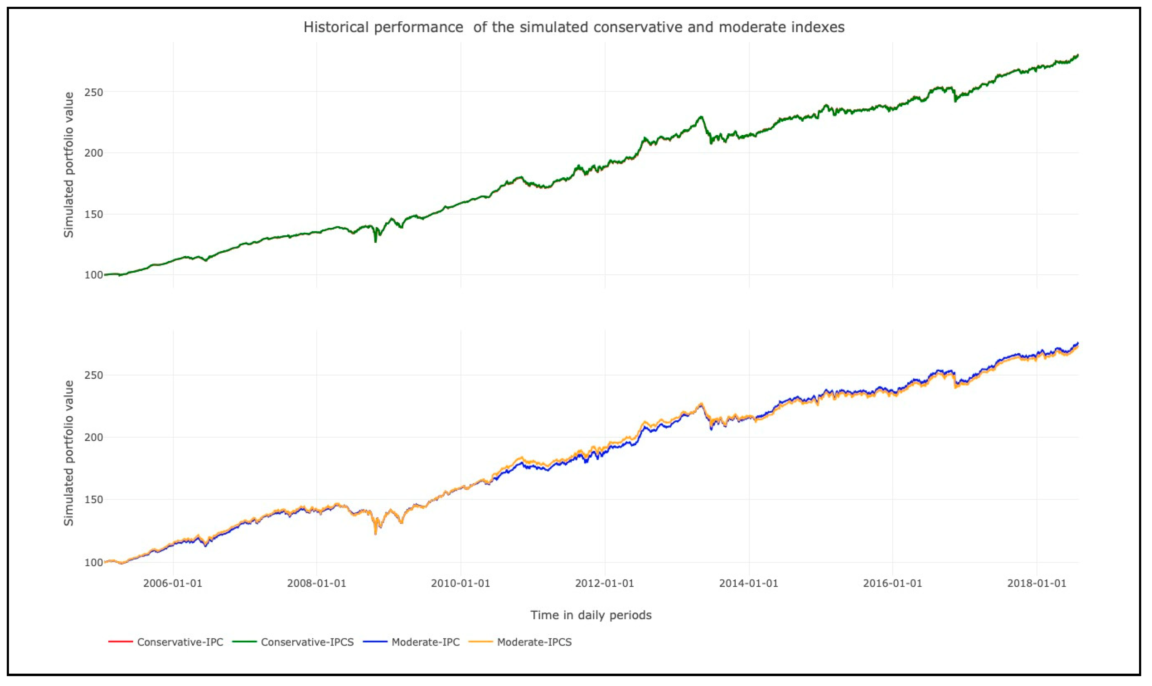
As a first result, we present in Figure 1 the historical (simulated) performance of the conservative (SB1) and moderate (SB2) target risk indexes given the investment levels of Table 3.

As noted, there was no significant difference in the performance of the simulated indexes for both types of SIEFOREs. Only the moderate-IPC showed differences, such as underperformance against the moderate-IPCS during the financial or Euro zone debt crisis time periods (mid 2006 to March 2008 and February 2010 to January 2014) and a marginal overperformance at the end of the simulation.

In practical terms, the conservative index that invests in the IPCS showed an accumulated return of 108.57% and the one that invested in the IPC, 108.27%. This result suggests that it is recommendable to use SRI in this specific case or risk profile without the significant loss of performance. We state this by the fact the difference in accumulated return was marginal and slightly in favor of the conventional investment style. Also, by referring to the performance in

Table 5. Accumulated returns and observed Sharpe ratio (with the accumulated returns).

Simulated index	Sharpe Ratio	Accumulated Returns (%)	Return Standard Deviation (%)
Conservative-IPC	2.2909	180.5762 [19.0862]	0.2732 [5.1844]
Conservative-IPCS	2.2848	180.2798 [19.0548]	0.2733 [5.1846]
Moderate-IPC	1.7859	175.5174 [18.5515]	0.3347 [6.3511]
Moderate-IPCS	1.6963	173.1464 [18.3009]	0.3446 [6.5389]
Growth-IPC	1.6185	173.9851 [18.3895]	0.3641 [6.9079]
Growth-IPCS	1.5146	171.0213 [18.0762]	0.3781 [7.1747]
Agressive-IPC	1.3624	184.5029 [19.5012]	0.4755 [9.0227]
Agressive-IPCS	1.1998	178.5754 [18.8747]	0.5124 [9.7228]
CETES28D	---	68.2067 [7.2092]	0.0055 [0.1035]

Source: Own elaboration with data of the simulations.

, we observe that the yearly accumulated return, standard deviation, and mean-variance efficiency (Sharpe ratio) were practically similar, leading us to suggest that it is preferable to have an SRI only investment policy in the local equity component of SB1 SIEFOREs.

For the case of type 2 SIEFOREs (SB2), the moderate indexes, it is noted that the performance showed some short-term differences, but at the end of the simulation, the simulated indexes showed an accumulated return of 175.51% for the case that invests in conventional Mexican equities and 173.14% for the SRI case. Similar to the previous type of index, we found no considerable difference between the mean return paid and the level of risk exposure (standard deviation) between the index that invested only in SRI stocks and the one that invested with a conventional strategy. Despite this, there was also a non-significant, but higher difference between the mean-variance efficiency of these two simulated indexes. The Sharpe ratio difference of the moderate-IPC with the moderate-IPCS was 0.0896. That means that for each extra 1% of risk level exposure in the moderate-IPCS, we would earn 0.08% less of the return above the risk-free rate than the moderate-IPC. As noted, the mean-variance efficiency loss was still small, as in the case of the conservative indexes that had a Sharpe ratio difference of 0.0061% of extra return lost for each 1% extra of risk exposure.

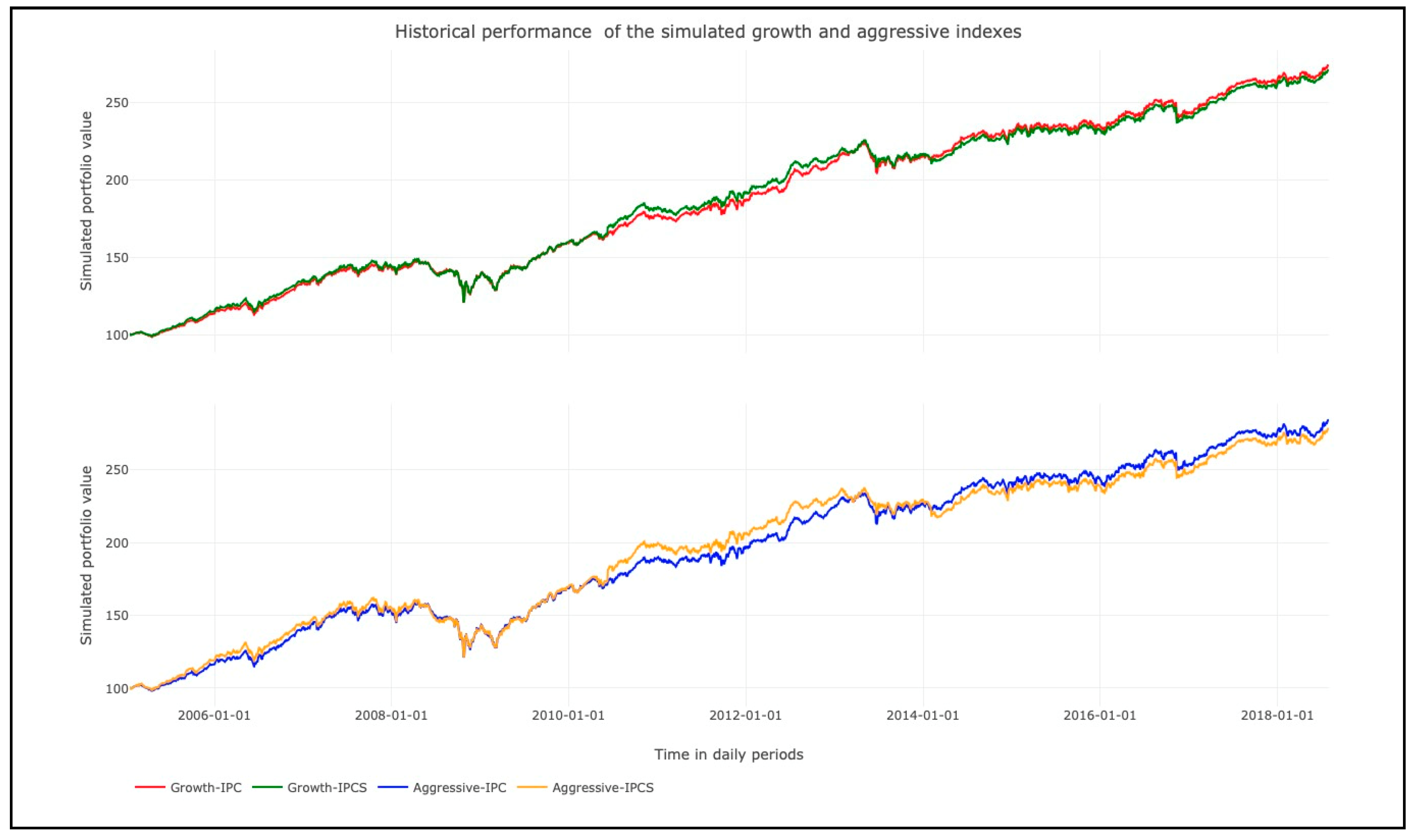
In Figure 2, along with the results shown in Table 5, we show the performance of the SB3 type SIEFOREs (growth indexes) and the SB4 (aggressive indexes) ones. In the first case, the short-term differences increased in relation to the SB2 SIEFORE type and the accumulated return at the end of the simulation. This can be noted by the fact that the accumulated gains were 173.98% for the SB3 (growth index) that invested in the IPC index and 171.02% for the case that invested in the IPCS (a 2.96% difference). Here, the short-term return loss was wider than in the previous type of SIEFOREs, but was still relatively low by the fact that the risk exposure (standard deviation) was just 0.2668% higher (in annual terms) in the growth-IPCS than in the growth-IPC. This result led to a Sharpe ratio or mean-variance efficiency loss (in relation with the growth-IPC) of only 0.1039% of extra return lost in the growth-IPCS (against the growth-IPC), given an extra 1% of risk exposure. As noted, in these three type of indexes, we cannot accept all of our particular hypotheses, (4) to (12), if we are numerically strict, but if we review our analysis in practical terms, the increase in risk exposure and the loss of expected (accumulated) return and Sharpe ratio was marginal and did not have a significant impact if these three types of public pension funds in Mexico perform an only socially responsible investment in their local equity component.

The same result, but with slightly wider differences in the short-term, is noted for SB4s (aggressive indexes) in the lower panel of Figure 2. The fluctuation of the SB4 that invested in the IPCS index was wider than the previously simulated ones. The accumulated earnings were 184.50% in the aggressive-IPC and 178.5% for the Aggressive-IPCS (a more notorious difference of 6%) and the risk exposure, in yearly terms, was 0.72%. With this wider accumulated return, but a marginally different risk exposure, the mean-variance efficiency loss of investing only in Mexican SRI stocks was of only 0.16%.

A result of interest from the previous results was the level of risk exposure of all the type of SIEFOREs that invested in Mexican SRI stocks (Table 5). These show a higher risk exposure in the cases that invested in the IPCS, a result that goes against the conclusions of De la Torre and Martinez [57], De la Torre et.al. [58], and De la Torre and Macias [5], who suggest that the performance of the IPCS sustainable index is statistically equal to the IPC comp and the IPC index. Even if this result is notable, the differences were practically marginal and we can summarize that even if we do not have strong proof to accept the null hypotheses (4) to (12), we also do not have strong proof to accept their alternative, leading us to suggest that the observed differences could be observed only in the short-term.

As a potential source of difference among the indexes that invested in the IPCS vs. the ones that invested in the IPC, is the fact that the base year in which De la Torre and Macias [5] recalculated the IPC sustainable index in a backward simulation was older than that used herein. This leads us to note that the accumulated return of the IPC index in the simulated period was 278.7238% vs. that observed in the IPCS of 258.0864%. If we multiply the difference of these accumulated returns by 20% (the investment level in the local equity factor for the aggressive or SB4 index), we arrive to the 5.92% difference between these two simulated benchmarks.

The other potential source of difference is the fact that the IPCS is more diversified in market capitalization size than the IPC, that is a blue-chip index. With this in mind, it is expected that the potential source of under-performance of the IPCS (that lead to this difference) is due to the fact that some small or mid-market capitalization stocks could have lagged behind the performance of the IPCS (and its corresponding target-risk indexes). In order to give support to our position on this matter, we present, in

Table 6. Performance attribution test of each simulated index.

Simulated Index	α	IPC Large Cap	IPC Mid Cap	IPC Small Cap	CETES
Conservative-IPC	−0.0002	---	---	---	0.0370 *
Conservative-IPCS	−0.0003	0.0163 ***	-0.0009	-0.0007	0.0366 *
Moderate-IPC	−0.0009	---	---	---	−0.0542
Moderate-IPCS	−0.0012	0.1316 ***	-0.0090 ***	-0.0048	−0.0586
Growth-IPC	−0.0011	---	---	---	−0.0679
Growth-IPCS	−0.0016	0.1642 ***	-0.0110 ***	-0.0059	−0.0716
Aggressive-IPC	−0.0019	---	---	---	−0.1209
Aggressive-IPCS	−0.0029	0.3097 ***	-0.0186 ***	-0.0109 *	−0.1168
Simulated Index	α	Udibonos	CORPOTRAC	Global 100	R-Squared
Conservative-IPC	0.1442 ***	0.5751 ***	0.2015 ***	0.0176 ***	0.9992
Conservative-IPCS	0.1456 ***	0.5730 ***	0.1996 ***	0.0168 ***	0.9982
Moderate-IPC	0.3759 ***	0.2726 ***	0.1811 ***	0.0712 ***	0.9929
Moderate-IPCS	0.3866 ***	0.2569 ***	0.1672 ***	0.0654 ***	0.9546
Growth-IPC	0.3357 ***	0.2622 ***	0.1898 ***	0.0898 ***	0.9915
Growth-IPCS	0.3493 ***	0.2429 ***	0.1717 ***	0.0824 ***	0.9419
Aggressive-IPC	0.2805 ***	0.2110 ***	0.1891 ***	0.0874 ***	0.9902
Aggressive-IPCS	0.3062 ***	0.1759 ***	0.1513 **	0.0731 ***	0.8943

Significance codes: 1% marked with ***, 5% with **, and 10% with *. Source: Own elaboration with data of the simulations.

, a regression of the performance attribution test in which we regressed (from 25 October 2006 to 31 July 2018, with a total of 2955 observations) the historical return time series of each simulated target risk index with the historical data of each type of assets index. For the local equity component (either IPC or IPCS), we divided it into three market cap indexes: The IPC large, mid, and small-cap benchmarks. These three benchmarks integrate the 60 stock members of the IPCcomp, which is the marker index benchmark from which the 35 members of the IPCS are screened. For the specific case of the simulated indexes that performed a conventional investment style (IPC), we performed the regression only with the large-cap index because the IPC has, as previously mentioned, only large-cap stocks.

As noted, only the growth and the aggressive target risk indexes were significant and negative in their β value. This was observed either in the mid cap or in the small cap indexes.

Despite this result, it is also noted that the riskiest simulated indexes that invested in the IPCS (growth or SB3 and aggressive or SB4) had a lower mean-variance efficiency and accumulated return. Despite this and given the analysis of Table 5 and Table 6, we can suggest that this difference is due only to the performance of mid and small cap stocks and holds only in the short-term.

The accumulated returns of the SB3 to SB4 type of SIEFOREs are in line with the results and conclusions of SRI given in the work of Derwall, Koedjik, and Horst [26] that suggest that the shunned-stock hypothesis holds. This is due to the fact that there was an observable underperformance in some simulated SRI portfolios against the ones that hold shunned, no-SRI stocks. Despite this, there is still proof to support the use of an only SRI strategy in Mexican pension funds. This may not lead to the creation of alpha, but to the value-driven quality of SRI (even if this means sacrificing performance marginally).

Given the last statement, we reviewed the performance not in a single regime time series, but in a two-regime one. The reason of this test was because we wanted to review the performance of this simulated indexes in bad-performing, distress, or crisis time periods. We used this nomenclature indistinctly (by following Hamilton [48,49,59,60,61]) to talk about the time periods in which the volatility levels in the financial markets of interest were higher. Our position is that the previous results do not filter the performance that each type of SIEFORE (target risk index) would have had, had they invested in the IPCS in distress time periods.

Departing this, we present in

Table 7. Goodness of fit test of the Gaussian single and two-regime scenarios.

Simulated Index	LLF 1 Regime	LLF 2 Regimes	Akaike 1 Regime	Akaike 2 Regimes
Conservative-IPC	15,271.71	15,990.80	−30,541.43	−31,975.60
Conservative-IPCS	15,271.63	15,978.66	−30,541.26	−31,951.32
Moderate-IPC	14,580.43	15,213.10	−29,158.86	−30,420.20
Moderate-IPCS	14,481.18	15,087.14	−28,960.35	−30,168.27
Growth-IPC	14,294.17	14,915.12	−28,586.34	−29,824.24
Growth-IPCS	14,165.10	14,772.32	−28,328.19	−29,538.64
Aggressive-IPC	13,384.53	13,981.98	−26,767.05	−27,957.96
Aggressive-IPCS	13,129.99	13,749.44	−26,257.97	−27,492.89
Simulated Index	Schwarz 1 Regime	Schwarz 2 Regimes	Hannan-Quinn 1 Regime	Hannan-Quinn 2 Regimes
Conservative-IPC	−30,535.29	−31,957.20	−30,538.78	−31,975.31
Conservative-IPCS	−30,535.12	−31,932.92	−30,538.61	−31,951.03
Moderate-IPC	−29,152.73	−30,401.80	−29,156.21	−30,419.91
Moderate-IPCS	−28,954.22	−30,149.87	−28,957.70	−30,167.98
Growth-IPC	−28,580.21	−29,805.84	−28,583.70	−29,823.96
Growth-IPCS	−28,322.06	−29,520.24	−28,325.55	−29,538.35
Aggressive-IPC	−26,760.92	−27,939.56	−26,764.41	−27,957.67
Aggressive-IPCS	−26,251.84	−27,474.49	−26,255.32	−27,492.60

Source: Own elaboration with data of the simulations.

the goodness of fit of the one and two-regime log-likelihood functions, (2) and (3), along with their information criterions. As noted in all the cases, there was a better fit to the data if the simulated indexes time series were described with a two-regime Markov-Switching model. With this goodness of fit result, we present in

Table 8. Statistical summary of the performance in the four simulated scenarios.

Simulated Index	Max Drawdown (%) 1 Regime	Mean Return (%) 1 Regime	Return Std. Dev. (%) 1 Regime	Sharpe Ratio (Mean Returns) 1 Regime
Conservative-IPC	−2.6435	0.0303 [10.9044]	0.2732 [5.1844]	1.0428
Conservative-IPCS	−2.6264	0.0303 [10.8932]	0.2733 [5.1846]	1.0407
Moderate-IPC	−3.2581	0.0298 [10.7121]	0.3347 [6.3511]	0.821
Moderate-IPCS	−3.4951	0.0295 [10.6207]	0.3446 [6.5389]	0.7835
Growth-IPC	−3.4274	0.0296 [10.6531]	0.3641 [6.9079]	0.7463
Growth-IPCS	−3.7251	0.0293 [10.5382]	0.3781 [7.1747]	0.7025
Aggressive-IPC	−3.9858	0.0307 [11.0513]	0.4755 [9.0227]	0.6155
Aggressive-IPCS	−4.5665	0.0301 [10.8287]	0.5124 [9.7228]	0.5483
CETES28D	---	0.0153 [5.4978]	0.0055 [0.1035]	---
Simulated Index	Max Drawdown (%) 2 Regimes	Mean Return (%) 2 Regimes	Return Std. Dev. (%) 2 Regimes	Sharpe Ratio (Mean Returns) 2 Regimes
Conservative-IPC	−0.4838/−2.6435	0.0386 [13.8979]/0.0070 [2.5036]	0.1524 [2.8916]/0.4671 [8.8627]	2.9050/−0.3378
Conservative-IPCS	−0.5008/−2.6264	0.0388 [13.9648]/0.0050 [1.7884]	0.1557 [2.9537]/0.4725 [8.9643]	2.8666/−0.4138
Moderate-IPC	−0.7576/−3.2581	0.0401 [14.4206]/−0.0118 [−4.2606]	0.2182 [4.1404]/0.6081 [11.5385]	2.1550/−0.8457
Moderate-IPCS	−0.7557/−3.4951	0.0386 [13.9087]/−0.0097 [−3.4889]	0.2278 [4.3215]/0.6354 [12.0560]	1.9463/−0.7454
Growth-IPC	−0.7423/−3.4274	0.0407 [14.6507]/−0.0128 [−4.5994]	0.2365 [4.4873]/0.6500 [12.3320]	2.0397/−0.8188
Growth-IPCS	−0.9669/−3.7251	0.0387 [13.9277]/−0.0123 [−4.4276]	0.2525 [4.7914]/0.7003 [13.2872]	1.7594/−0.7470
Aggressive-IPC	−1.1856/−3.9858	0.0412 [14.8275]/−0.0117 [−4.2208]	0.3178 [6.0291]/0.8543 [16.2084]	1.5474/−0.5996
Aggressive-IPCS	−1.337/−4.5665	0.0392 [14.1226]/−0.0129 [−4.6537]	0.3461 [6.5667]/0.9650 [18.3091]	1.3134/−0.5545

Source: Own elaboration with data of the simulations.

the max drawdown and mean-variance efficiency results in a single (as in Table 5) and two-regime scenario.

In order to determine if a given realization belonged to a given regime, we used the next rule: Δ%B_i,t,s=2 if P(s = 2|r_t, μ_s=i, σ_s=i, π_s=i, P) > 0.5 or Δ%B_i,t,s=1 if P(s = 2|r_t,μ_s=i,σ_s=i,π_s=I,P) ≤ 0.5. Please refer to Hamilton [39,41] and Hauptman et al. [62] for further reference.

We also show, in the same table, the risk or standard deviation levels, along with the Sharpe ratio as in (13) and mean expected returns.

In a two-regime perspective, the picture looks similar to the previous review in Table 5. The main difference arrives in the second regime (the bad-performing, distress, or crisis one). In this specific scenario, practically all the simulated indexes or SIEFORE types had a better expected return if they used the IPCS instead of the IPC. This last result goes in line with Areal, Cortez, and Silva [34], De la Torre and Martinez [57], and De la Torre and Macias [5] by the fact that the IPCS (SRI) had a better performance in crisis time periods.

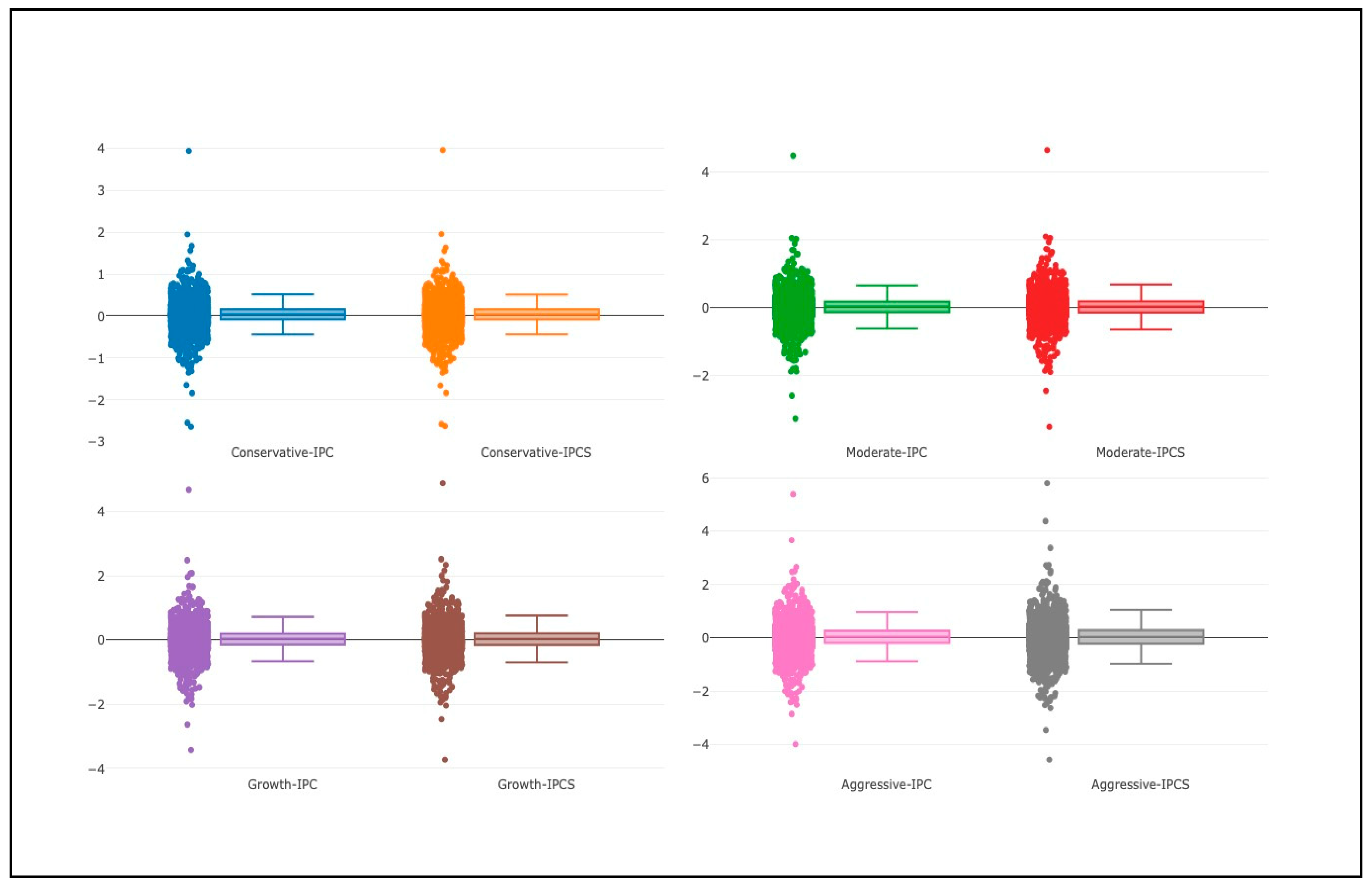
Finally, we present in Figure 3 a box plot of the percentage variations or returns of the simulated type of SIEFOREs (or indexes). From a paired perspective in each SIEFORE type and by paying attention to the 95% confidence interval boxes, it is noted that the use of the IPCS did not dramatically change the behavior of the performance of a SIEFOREs type 1 to type 4. By making a review of the pair of box plots, it is noted that they practically have the same shape, but the performance of the individual returns showed more extreme outliers in some specific dates. These extreme returns give a stronger support to our position that the observed differences between the four pairs of simulated indexes are observed only in the short-term and the expected (mean) return and risk (standard deviation) differences are due to these short-term outliers and not to a systematic poor performance of SRI.

As a corollary of results, we can mention that even if there is weak proof to accept all the proposed null hypotheses (if we are numerically strict), the results of Table 5 and Table 7, the performance attribution test of Table 6, the Markov-Switching model of Table 8, and Figure 3 suggest that even if there is a marginal “under-performance” in the short-term, this does not hold in the long-term. Also, we can suggest that investing in SRI is much better for Mexican public pension funds in distress or bad-performing time periods, such as the ones observed in 2007-2008 (just to give a significant example in our simulation period).

4. Conclusions

Socially responsible investment (SRI) is a practice that has evolved since its ancient origins to the actual applications that started as activist investing in the 1970s. The evolution of it suggests SRI as a new type of investment style that is being accepted as such in the investment industry. As a result of this evolution and acceptance, several studies have been made to test the appropriateness of the risk, return, or utility maximization for the individual or institutional investor. One of the main issues of SRI is that it leads to less diversified portfolios than conventional ones (portfolios with SRI and non-SRI stocks), having an impact in the mean-variance efficiency and, potentially, in the utility maximization and performance. Departing from the literature review of these studies, it is noted that little has been written about the benefits that SRI has had for institutional investors, such as public pension funds. With this in mind, this study extended the work of De la Torre and Macias [5], who tested the mean-variance efficiency in the Mexican public pension funds (known as SIEFOREs) by testing the mean-variance efficiency achieved in the S&P/BMV target-risk Mexico indexes had these invested only in SRI in the Mexican equity component.

The Mexican Public pension system is one with a life-cycle investment style in which there are four types of pension mutual-funds (known as SIEFOREs), with type 1 (SB1) being the most conservative (focused on pension savers close to retirement with an age of 59 years or less) and type 4 (SB4) the most aggressive, focused on investors of 36 years of age or less. Departing from this, we simulated the performance of the four S&P/BMV target-risk benchmarks (one for each SIEFORE type) by making a historical simulation of the investment policy of these, and by changing in one scenario the use of the S&P/BMV IPC index (IPC) with the S&P/BMV IPC sustainable (IPCS) in the Mexican equity component. The results showed that there was no significant mean-variance efficiency loss in type 1 (SB1) SIEFOREs and potentially also in type 2 (SB2) and type 3 (SB3). However, in the most aggressive type 4 (SB4), there was a wider difference in the short-term. This loss of mean-variance efficiency is due to the performance of the small and mid-cap stocks that are members of the IPCS and its performance lag against the IPC (conformed of large-cap stocks only).

Even if there is a performance and mean-variance efficiency loss in the most aggressive type of pension funds, this loss is marginal and, in practical terms, does not have a significant impact in the long-term. Departing from this result, we suggest to the Mexican pension authorities (CONSAR) to promote a SRI only strategy in the local equity component of the Mexican public pension funds without the loss of significant performance and mean-variance efficiency.

By performing a two-regime analysis with a Gaussian Markov-switching model, we found that, in line with the previous literature, in the Mexican SRI case, it is also preferable to invest in SRI Mexican stock in distress time periods.

Finally, we made a visual inspection of the performance of each simulated index and we found proof to observe that the mean-variance efficiency loss was due to outliers or extreme positive and negative movements of the IPCS and not due to a systematic under-performance of the IPCS against the IPC.

The results from the current research also suggest that the shunned-stock hypothesis suggested by Derwall, Koedjik, and Horst [26] holds in this particular case. With this in mind, the not-so-equal performance achieved by investing the procedures of Mexican pension funds in Mexican SRI stocks could be a value-driven one and the potential efficiency loss could be due to the higher prices of SRI stocks (compared with the ones of the shunned or non-SRI stocks).

Following this last statement, a potential guideline for further research could be a more proper test of the aforementioned shunned-stock hypothesis in the Mexican case, and the test of the simulation with other SRI stock indexes and their market factor performance tests. Another guideline could be the application of this test in the multi-asset investment policy of pension funds outside Mexico and to test the implications of an ESG only strategy in these funds and in another type of institutional investor.

Finally, our last recommendation is for policy makers (either Mexican or international pension saving authorities): Given our results, we suggest promoting an SRI only strategy in the public Mexican pension funds by the fact that even if we found under-performance against the conventional investment strategy, this underperformance is a short-term one and, in the long-term, the benefits of investing in SRI companies is not only for pension savers, but for their entire economy. We make this suggestion because SRI companies could have lower market price cost or credit rates, as incentives to improve the environmental and social impact of their activities.