Evaluation of the Effects of a Machine Failure on the Robustness of a Job Shop System—Proactive Approaches

Abstract

Researchers are searching for opportunities to organize production systems that save energy and natural resources. Preventive maintenance (PM) is essential for the efficient use of machines and energy saving. Any rework due to a machine failure consumes additional energy, human resources, equipment, spare parts and raw materials. Two criteria—quality robustness (QR) and solution robustness (SR)—are used in order to compute the operational efficiency of the production system in the event of disruption. Any cost criterion can be added to the QR in order to measure losses due to a machine failure. The SR criterion measures a number of changes necessary to adopt the production schedule after the machine failure. Two proactive approaches are compared to compute the operational efficiency. In the predictive-reactive approach, the PM time is predicted and a stable schedule is built. In the proactive-reactive approach, a schedule is achieved for the best sequence of idle times between jobs. The influence of disturbance on both schedules using robustness measures is examined. This paper presents the results of computer simulations for the above approaches. The approaches are compared in order to select a better method of production organization that reduces costs and waste due to machine failure.

1. Introduction

Real-life situations relate to a new way of doing business and creating value by “sustainable manufacturing”. Researchers are searching for production systems that minimize negative environmental impacts, conserve energy and natural resources, are safe for employees, communities and consumers, and are economically sound.

Energy saving is a key factor resulting from the need to reduce costs, use limited resources efficiently and be environmentally friendly. Preventive maintenance (PM) is essential for the efficient use of machines and energy saving. Any rework due to a machine failure consumes additional energy, human resources, equipment, spare parts and raw materials. Additional energy is consumed by adapting of a shop floor in accordance with the schedule changes. Additional set-up operations are carried out for machines. Additional organizational changes of human resources and raw materials requirements are also necessary. In other words, the fewer changes in the adopted schedule, the greater the energy savings. A stable and reliable schedule can be obtained using predictive methods for determining PM time. Building a schedule for production and maintenance jobs helps in the creation of manufacturing processes that minimize negative environmental impacts, conserve energy and natural resources, and are economically sound. The number of changes made to the schedules after the disturbance (the bottleneck failure) is measured using the criteria of quality robustness and solution robustness. Quality robustness measures the degradation of the performance of the schedule due to the disturbance. Solution robustness measures the sum of absolute deviations of operation start times in the reactive and basic schedules. The impact of machine failures must be minimized.

Preventive maintenance is carried out in order to keep the production system at the high level of operation due to restricted resources. The main idea of PM is to prevent failures before they occur. Some papers search for a method that minimizes the probability of failure. Other papers search for a method that minimizes the impact of failure on a schedule. The first group of methods belongs to predictive scheduling. The second group of methods belongs to proactive and reactive scheduling. Both groups are important in real-life situations. The following literature review is carried out taking into account the above research groups.

1.1. Literature Review

First, the pros and cons of predictive, proactive and reactive scheduling methods are determined. The main idea of predictive scheduling is to introduce maintenance into a schedule in order to increase the probability of running the schedule without disturbances. In predictive scheduling, researchers assume that PM performed at regular intervals is enough for machines to be available and reliable [1]. Some researchers assume that the time to implement preventive maintenance is flexible. Certain flexibility is obtained by giving each maintenance task a time window in which the actual start time of the maintenance can move [1,2]. However, more reliable methods are based on inserting a time buffer for maintenance prior to a job with a disturbance prediction [3].

In proactive scheduling, the impact of an unexpected machine failure over the performance of the production system is investigated. A common feature of the proactive scheduling methods is that researchers advocate schedule robustness to deal with uncertainty. A schedule that best deals with the disturbance is accepted for action. There are two types of schedule assessment measures: robustness of a solution and robustness of the solution quality. Solution robustness measures the insensitivity of the operation start times to variations in the input data. Quality robustness measures the insensitivity of objective functions due to disruptions [4]. Proactive scheduling methods differ in their strategy of reducing the impact of uncertainty. Some researchers use prediction methods in order to predict time of PM and built predictive schedules. Next, the influence of the disturbance on the predictive schedule using the robustness measures is examined. This approach is called predictive-reactive (proactive with prediction) [5,6,7]. Some researchers simply investigate the impact of disruption on a proactive schedule using robustness criteria. But the proactive schedule is achieved for the best sequence of idle times between jobs or batches taking advantage of the simulation process. This approach is called proactive-reactive (proactive without prediction) [8,9,10]. Predictive-reactive and proactive-reactive approaches are implemented at the decision stage. It is necessary to compare predictive-reactive and proactive-reactive approaches and this is the subject of this paper.

In reactive (dynamic) scheduling, the impact of frequency and method of rescheduling over the performance of a production system is investigated. Researchers investigate when and how to respond to real-time events [11]. The efficiency of rescheduling techniques is assessed using robustness criteria. Reactive scheduling is carried out at runtime to adjust the schedule to the real-time situation.

The author of this paper intends to compare proactive-reactive approaches with predictive-reactive approaches. Thus, the literature review is continued considering these two groups.

First, proactive-reactive approaches are considered. Lei [12] considered PM as an availability constraint but there is no explanation of how the PM time is determined. Each maintenance operation has a fixed predefined time interval. The beginning times of operations are fuzzy. The author examined the impact of PM time on the completion times of jobs. He proved that “most of the possible actual completion times lie in the cut of fuzzy completion time for each job.” [12]. Bali and Labdelaoui [13] searched for a maintenance schedule that guarantees a high level of system reliability and reduces both maintenance resources and power demand. The time horizon of the schedule is divided into periods in which maintenance operations are performed. The authors examine the impact of starting times of maintenance, for each unit of the power system, on constraints of the problem. The first constraint imposes a continuous and limited maintenance window for each unit of the power system. The second constraint imposes a limited total number of maintenance crew available for each scheduling period. The third constraint imposes a limited capacity of the running units at each period of the maintenance schedule. The capacity should not be less than the predicted load demand at given period.

Considering only the relationship between production and maintenance as a conflict in management decisions may result in unsatisfied demand or machine breakdowns. A common objective is to maximize system productivity and efficiency. Moreover, the time interval of PM activities and the number of PMs are usually pre-known and fixed in advance. In the proactive–reactive approaches, reliability analyses need to be applied to handle the maintenance aspect. The mentioned deficiencies in the proactive-reactive approaches are the advantages in the predictive-reactive approaches.

Next, predictive-reactive approaches are considered. Mokhtari et al. [14] searched for the best allocation of jobs for machines in order to satisfy the predefined makespan value as well as PMs in order to minimize unavailability of the production system. The advantage of the proposed method is the description of a machine condition using the availability function. Unavailability of the machine is zero at the beginning of the scheduling horizon. Availability of the machine is deteriorated with the maximum repair rate predefined for the machine. The machine is restored to the “as good as new” condition after PM. PM time is determined for each machine in order to maximize the availability of the production system. By using the availability component in the objective function, the algorithm assigns PMs in intervals that increase the availability of machines. But the searching process is longer because the neighborhood search algorithm is based on random insertion and swap moves. The disadvantage of this method is the lack of prediction of the time of machine unavailability. Bajestani et al. [15] searched for the best allocation of jobs and PMs for machines in order to minimize the total cost of maintenance and lost production. Two cases are considered: a machine is maintenance-free and the machine needs maintenance. In the first case, the state of the machine and its production rate are known at the beginning of a time period. The transition probability in which the machine changes its state at a given time is predefined. The probability that a machine is in a given state at the start-time of a job depends on both the condition of the machine and the time of maintenance. The disadvantage of the proposed method is that maintenance is performed with a negligible time at the beginning of each time period. The machine is maintained only when it is in a state of failure and as a result, there is no production at the beginning of the next period. The average production rate of the machine depends on its state given at the beginning and at the end of the period. And the average values are described by given time intervals (uniformly distributed) with no historical analysis. In the paper [16] the idea of predictive-reactive scheduling of production tasks is outlined. Predictive scheduling is proposed for a production process with two uncertainties: unknown machine failure times and variability of task processing times. A possible machine failure is introduced as a buffer time (for maintenance) with a fixed duration in the production model. The time of failure is pre-determined for each machine. Failure times are selected based on the assumption of the largest number of tasks processed on machines at that time. The advantage of the method is that the lengths of time buffers are supported by the technical data issued by the maintenance department of a given manufacturing company.

Taking into account machine conditions allows for more efficient use of potential production time. Some predictive-reactive approaches use probability theory to describe machine conditions. Other predictive-reactive approaches assume only a fixed period of unavailability of machines for technical service. However, accepting the assumption that machine conditions are observable at the beginning of each period is not sufficient. Recently, the problems of production scheduling with disturbances have become more and more popular in the scientific community. The most popular machine maintenance strategies are based on the periodic inspection of a machine and age dependent inspection. Researchers should use predictive methods to analyse historical failure-free times. Attributes to describe a machine age and the influence of maintenance should be drawn from analysis of historical data [7,17].

The advantages of the predictive-reactive method used in this paper are four-fold:

• The predictive-reactive approach uses historical data analysis for PM time prediction;
• Preventive maintenance of the bottleneck is planned in order to reduce unexpected failure;
• Flexible operations are allocated to the bottleneck during a higher probability of failure in order to increase the robustness of the schedule;
• The computer simulation is used to determine the start time of operations on machines in a balanced schedule for robustness criteria.

1.2. Goals and Approaches

It is necessary to examine the following research point—which construction of proactive algorithms achieves better solutions: proactive-reactive (proactive without prediction) or predictive-reactive (proactive with prediction). The first construction consists in repeating the closed loop: the set of task sequences is obtained in the coding procedure, trained in the affinity maturation procedure and evaluated after the decoding procedure. The quality of a schedule depends on the impact of the disruption on criteria: the makespan C_max, total tardiness T, total flow-time F, total idle time of machines I, and stability criterion SR. The second construction consists in repeating the closed loop: a population of the task sequence is generated, the sequence is rebuilt using the minimal impact of disrupted operation on the schedule MIDOS rule in order to make the schedule more robust. In the MIDOS rule, PM is assigned to the bottleneck at the time of predicted failure. Estimation methods of the mean time to failure and other reliability characteristics are presented in [7,17]. Next, the sequences of production and maintenance tasks are trained and evaluated taking into account the effects of the machine failure on criteria: C_max, T, F, I and SR. Taking into account the reliability information of a critical machine some predictions are added in the second construction. Both approaches are compared using the multi-objective immune algorithm described in the next section.

The original contribution to the existing state of research is the comparison analysis of proactive methods using not only the advantage of computer simulation but also prediction. Bearing in mind the review of the literature, the research points are defined:

• Approaches of dealing with the machine failure and obtaining the best proactive schedules, when the objective is to minimise criteria: C_max, T, F, I.
• Methods dealing with anticipated or unanticipated disruptions, that maximize robustness criteria: SR and QR.

The paper is organized as follows: two constructions of proactive algorithms—proactive-reactive (proactive without prediction) and predictive-reactive (proactive with prediction)—are presented in the next section. The criteria for the assessment of predictive and reactive schedules are also described in Section 2. The mathematical model of the production system with disruptions (a machine failure) is presented in Section 3. The job shop scheduling problem, together with interruptions for experimental study, is presented in Section 4. Section 5 contains necessary analyses and experimental test results related to the research on the application of proactive algorithms in the job shop problem. The paper concludes with a brief summary of the results (Section 6).

2. Two Proactive Approaches Using the HMOIA

Originally, the multi-objective immune algorithm (MOIA) was applicable to solve deterministic (basic) scheduling problems [18,19,20].

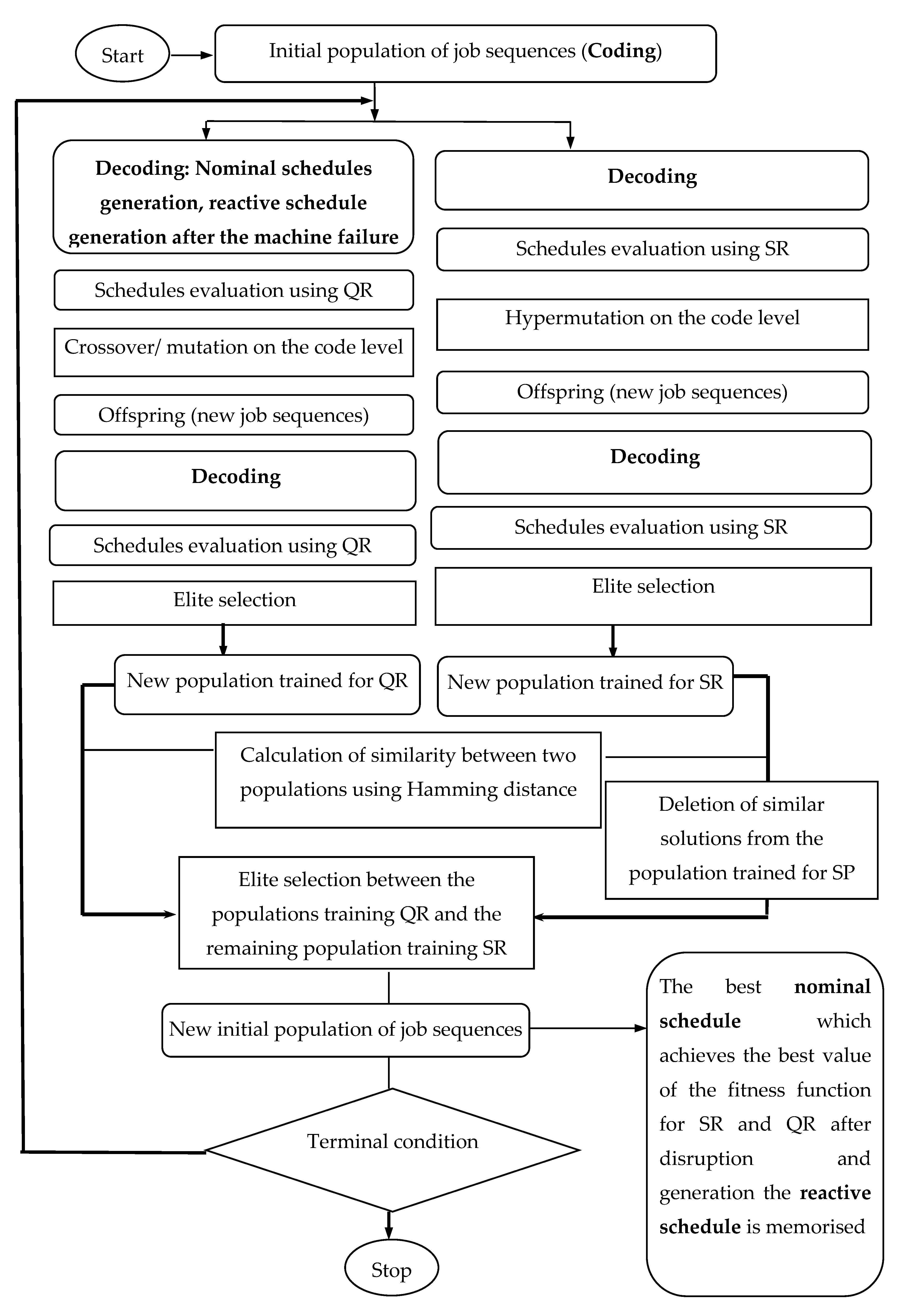
Next, modification of the MOIA was applied to solve proactive-reactive scheduling problems [21]. The modification is called the hybrid multi-objective immune algorithm II (HMOIA II). The HMOIA II searches the solution space for the most stable and robust solutions. The algorithm repeats the procedures: coding solutions, training solutions, decoding solutions, evaluating solutions and eliminating similar solutions (Figure 1). The algorithm effectively scans the solution space to achieve the most robust schedule (Fig.1 in [21]). Solutions are evaluated using two criteria: solution robustness (SR) and quality robustness (QR). QR measures how much the quality of the basic schedule has deteriorated after the disruption. SR measures the sum of absolute deviations of operation start times in the reactive and nominal (basic) schedule. The fitness function adds the weighted values of QR and SR. The criteria are equivalent.

The elite selection is used to select a better solution from a pair: parent and offspring. Solutions with lower values of the fitness function create a new initial population in the next iteration. In each iteration, the best solution is copied to the immune memory. It means that the job sequence will best deal with disruption (Figure 1). In HMOIA II, the training process is terminated with a given number of iterations.

“The training process of antibody population for QR starts with antibodies selection to create a mating pool. Parents are randomly matched in couples.” [21] (Figure 1). Mutation and crossover procedures are used to train the population of solutions for QR [21]. Hypermutation procedure is used to train the population of solutions for SR [21].

In order to maintain a high diversity of solutions trained in subpopulations for QR and SR, the Hamming distance is calculated for each solution. Affthres is a threshold value that determines the similarity of two solutions. “An antibody is deleted from the population trained for the SR if it is stimulated by a number of antibodies more than stimthres.” [21]. The removed antibody is replaced by an antibody with the same index from the population trained for SR.

After the terminal condition is met, the best solution is selected from the immune memory.

In [21], authors proposed the construction of the algorithm to achieve the best compromise solution for SR and QR. In this paper, the decoding process is differentiated in two approaches: proactive-reactive (proactive without prediction) or predictive-reactive (proactive with prediction) (Figure 2 and Figure 3).

In the first approach (HMOIA II), a job sequence is decoded by generating the nominal schedule (with deterministic input data), then, the reactive schedule is generated after the bottleneck failure (Figure 2). In the second approach (HMOIA III), a job sequence is decoded by generating the basic (nominal) schedule. The basic schedule is then rebuilt using the MIDOS rule in order to generate a predictive schedule [22]. The MIDOS rule assigns a preventive maintenance task at the predicted time of the bottleneck failure. Then the most flexible task operations are assigned during the high probability period of failure. The MIDOS rule makes the schedule more robust and flexible in the event of the bottleneck failure. The reactive schedule is generated after the bottleneck failure (Figure 3).

The proactive scheduling approaches differ in their strategy of reducing the impact of uncertainty. The first approach (HMOIA II) simply investigates the impact of disruption on a nominal schedule using robustness criteria. But the proactive schedule is achieved for the best sequence of jobs taking advantage of the simulation process. The second approach (HMOIA III) uses prediction methods [7,17] in order to predict time of PM and built a predictive schedule using the MIDOS rule. Then, the influence of the disturbance on the predictive schedule using the robustness measures is examined.

Computer simulations are run for the two proactive approaches for the job shop scheduling problem and reliability characteristics presented in Section 4. First the mathematical model of the production system with disruptions (a machine failure) is presented.

3. The Mathematical Model of the Production System with Disruptions

A job shop scheduling problem with disturbance is described by J tasks (j = 1,2,…, J) that are to be scheduled on W machines (w = 1,2,…, W). Each production task is represented by a number of non-pre-emptive operations V_j which is equal to the number of machines (v_j = 1,2, …, V_j). The execution of operation v_j of task j requires a machine according to a technological route. Operation v_j occupies predefined machine time units. After the machine failure, operation v_j requires one machine selected from a set of parallel machines. Processing time $a_w{,}_{v_j}$ of operation v_j is non-resumable after a disruption (the bottleneck failure). It means that operation v_j must be reprocessed fully after repair of the bottleneck.

The maintenance task must be performed on the most occupied machine in every planning horizon. The production system with disturbances (bottleneck failures) is monitored in order to collect information on a number of disruptions, disruption-free times and repair times. It is assumed that successive disruption-free times are assumed to have Weibull distributions and are followed by exponentially distributed times of machine service (repair). It was observed that parameters of these distributions change with time. Based on the collected information in a number of planning horizons of the same duration in the past predictions of the reliability characteristics are estimated. Such a production system, firstly, is observed on m successive planning horizons:

$$\left[0,T\right),\left[T,2T\right),\dots ,\left[\left(m-1\right)T,mT\right)$$

(1)

of the same duration, for which information about numbers of disturbances or disturbance-free times is collected. The prediction of job shop system operation is being built for the next planning horizon $\left[mT,\left(m+1\right)T\right)$. Disturbance-free times $X_{i,1},\dots ,X_{i,N_i}$ in the ith planning horizon $\left[\left(i-1\right)T,iT\right),i=1,\dots ,m+1$ have a Weibull distribution with probability density function $f_i(\cdot )$ of the form:

$$f_i\left(t\right)=\{\begin{array}{l}{\lambda }_i{p}_i{t}^{p_i-1}exp\left(-{\lambda }_i{t}^{p_i}\right),t>0,\\ 0,t\le 0,\end{array}$$

(2)

where $p_i>0,{\lambda }_i>0,$ thus parameters of the distribution depend on the number of period and are the same in each period separately. Here $N_i$ denotes a random number of failures detected in $\left[\left(i-1\right)T,iT\right)$.

At the end of reliable work period $X_{i,k}$, as the failure occurs, a repair time $Y_{i,k}$ begins immediately and so on. Repair times $Y_{i,1},\dots ,Y_{i,N_i}$ for $i=1,\dots ,m+1$ are supposed to be exponentially distributed with probability distribution functions PDFs $g_i(\cdot )$ of the form:

$$g_i\left(t\right)=\{\begin{array}{l}{\alpha }_{i}exp\left(-{\alpha }_{i}t\right),t>0,\\ 0,t\le 0,\end{array}$$

(3)

Assuming that numbers and durations of successive disturbance-free periods have been measured and are known for each planning horizon, parameters of distributions $f_i(\cdot )$ are estimated using the maximum likelihood approach or empirical moments approach.

3.1. Maximum Likelihood Approach

Assuming that in each of planning horizon $\left[0,T\right),\left[T,2T\right),\dots ,\left[\left(m-1\right)T,mT\right)$ disturbance-free periods $X_{i,k},$ $k=1,\dots ,N_i$ for any $i=1,\dots ,m$ are given, where $n_i$ is the observed value of $N_i$, thus the observations are described by:

$$\left(x_{1,1},x_{1,2},\dots ,x_{1,n_1}\right),\dots ,\left(x_{m,1},x_{m,2},\dots ,x_{m,n_m}\right)$$

(4)

Consider firstly the planning horizon $\left[0,T\right)$. $x_{1,1},x_{1,2},\dots ,x_{1,n_1}$ are independent and identically distributed collected variables. Unknown parameter $p_1$ of Weibull distribution is estimated using the following equation [23]:

$$n{\displaystyle \sum }_{k=1}^{n_1}{x}_{1,k}^{p_1}ln{x}_{1,k}-\left(\frac{n_1}{p_1}+{\displaystyle \sum }_{k=1}^{n_1}ln{x}_{1,k}\right){\displaystyle \sum }_{k=1}^{n_1}{x}_{1,k}^{p_1}=0.$$

(5)

Obtaining estimated value of $\widehat{p_1}$ unknown parameter ${\lambda }_1$ of Weibull distribution is estimated just from the following equation:

$$\widehat{{\lambda }_1}=\frac{n_1}{{{\displaystyle \sum }}_{k=1}^{n_1}{x}_{1k}^{\widehat{p_1}}}.$$

(6)

After achieving estimators $\widehat{p_1},\dots ,\widehat{p_m}$ and $\widehat{{\lambda }_1},\dots ,\widehat{{\lambda }_m}$ one can extrapolate values ${\widehat{p}}_{m+1}$ and ${\widehat{\lambda }}_{m+1}$ for the next planning horizon $\left[mT,\left(m+1\right)T\right)$ for which we have no observation, using the regression method.

3.2. Empirical Moments Approach

Assume that there are disturbance-free periods $x_{1,1},x_{1,2},\dots ,x_{1,n_1}$ for planning horizon $\left[0,T\right)$ as in the previous section. Analyzing the behavior of the condition [23]:

$$T_1\left(\frac{1}{p_1}\right)=\sqrt{\frac{\pi }{p_1}}\cdot {\left(\frac{1}{4}\right)}^{\frac{1}{p_1}}$$

(7)

for fixed value $T_0=\frac{m_1^2\left(x_1\right)}{m_2\left(x_1\right)}$, one can find an approximate value $\widehat{p_1}$ of $p_1$. Here $m_1\left(x_1\right)$ denotes disturbance-free mean and $m_2\left(x_1\right)$ is the second moment as follows:

$$m_1\left(x_1\right)={\overline{x}}_1=\frac{1}{n_1}{{\displaystyle \sum }}_{k=1}^{n_1}{x}_{1,k}, m_2\left(x_1\right)=\frac{1}{n_1}{{\displaystyle \sum }}_{k=1}^{n_1}{x}_{1,k}^2$$

(8)

Having $\widehat{p_1}$ one can obtain an approximate value $\widehat{{\lambda }_1}$ of ${\lambda }_1$ just from the equation:

$$\widehat{{\lambda }_1}={\left[m_1\left(x_1\right)/\Gamma \left(\frac{1}{\widehat{p_1}}+1\right)\right]}^{-\widehat{p_1}}$$

(9)

The exact value of ${\lambda }_1$ is impossible to obtain just from the above equation. One method of approximation uses the Gamma function:

$$\Gamma \left(x+1\right)\approx x^{x+\frac{1}{2}}{e}^{-x}{e}^{\frac{1}{2}ln2\pi },x\to \infty$$

(10)

After obtaining estimators $\widehat{p_1},\dots ,\widehat{p_m}$ and $\widehat{{\lambda }_1},\dots ,\widehat{{\lambda }_m}$ one can extrapolate values ${\widehat{p}}_{m+1}$ and ${\widehat{\lambda }}_{m+1}$ for the next planning horizon $\left[mT,\left(m+1\right)T\right)$ for which we have no observation, using the regression method.

3.3. Reliability Characeristics

Let us consider planning horizons $\left[\left(m-1\right)T,mT\right)$ for which estimators ${\widehat{p}}_{m+1}$ and ${\widehat{\lambda }}_{m+1}$ of Weibull distribution were obtained (using one of two methods). Below the formulae for the reliability characteristics used in the MIDOS rule are given:

• The maintenance task is assigned to the bottleneck at the time determined by the mean time between failures (MTBF)

  $$MTBF=E\left\{X_{m+1,1}+Y_{m+1,1}\right\}={\left(\frac{1}{{\widehat{\lambda }}_{m+1}}\right)}^{\raisebox{1ex}{$1$}\!\left/ \!\raisebox{-1ex}{${\widehat{p}}_{m+1}$}\right.}\Gamma \left(\frac{1}{{\widehat{p}}_{m+1}}+1\right)+\left(\frac{1}{{\alpha }_{m+1}}\right),$$

  (11)

  where: ${\alpha }_{m+1}>0$ is predefined.
• The risk of inconsistent prediction of machine failure-free time is minimized by assigning the most flexible operations to the period limited by points b and a, where:
  a is estimated on the assumption [7] that the probability of the failure-free time of the bottleneck described by the Weibull distribution with parameters ${\widehat{p}}_{m+1}$ and ${\widehat{\lambda }}_{m+1}$ is higher than a equalling 40%, $P\left\{X_{m+1,1}>a\right\}=0.4$.
  Thus, $P\left\{X_{m+1,1}<a\right\}=0.6$ and $1-e\left(-\lambda \cdot a^p\right)=0.6$, and we have $e\left(-\lambda \cdot a^p\right)=0.4$ and taking the property $lne\left(r\right)=r$ we achieve $a^p=-ln\left(0.4\right)/\lambda$ and finally:

  $$a=\sqrt[p]{-ln\left(0.4\right)/\lambda }$$

  (12)
  b is estimated on the assumption that the probability of the failure-free time of the bottleneck described by Weibull distribution with parameters ${\widehat{p}}_{m+1}$ and ${\widehat{\lambda }}_{m+1}$ is less than b equalling 70%, $P\left\{X_{m+1,1}<b\right\}=0.7$ thus
  $1-e\left(-\lambda \cdot b^p\right)=0.7$ and we have $e\left(-\lambda \cdot b^p\right)=0.3$ and taking the property $lne\left(r\right)=r$ we achieve $b^p=-ln\left(0.3\right)/\lambda$ and finally

  $$b=\sqrt[p]{-ln\left(0.3\right)/\lambda }$$

  (13)

Having the above reliability characteristics, a flexible schedule is generated using the MIDOS rule. The achieved schedule is evaluated before and after the disturbance.

3.4. Evaluation Criteria

The job shop scheduling problem with disturbance is formulated to schedule a set of production tasks to a set of machines subject to the following constraints:

• the operation sequence of a production task is predefined;
• operations of production tasks are pre-assigned to machines according to technological routes;
• the disturbed operation can be rescheduled to one machine from a set of parallel machines;
• preventive maintenance of the bottleneck has to be completed at the time of the MTBF.

The objective is to minimise the following criteria of predictive schedule x:

• Makespan of production tasks:

  $$F_1=min C_{max\left[t_{z,V_j}\right]max}$$

  (14)

  where: $t_{z,v_j}$ is completion time of operation $v_j$ of task j, $v_j=1,\dots ,V_j$, $j=1,\dots ,J$;
• Flow time of production tasks:

  $$F_2=min F={\displaystyle \sum }_{j=1}^J\left(t_{z,V_j}-t_{r,1_j}\right)$$

  (15)

  where: $t_{r,v_j}$ is start time of operation $v_j$ of task j;
• Total tardiness of production tasks:

  $$F_3=min T={\displaystyle \sum }_{j=1}^J\left[0,D_j\right]$$

  (16)

  where: $\{\begin{array}{c}0,\hspace{1em}if d_j-t_{z,V_j}\le 0\\ D_{i,\hspace{1em}}if d_j-t_{z,V_j}>0\end{array}$
  and $d_j$ is deadline for completing task j; D_j is delay in completing task j.
• Idle time of machines:

  $$F_4=min I={\displaystyle \sum }_{w=1}^W{I}_w$$

  (17)

  where I_w is idle time of machine w, $w=1,\dots ,W$.
• The weighted sum of values of the four objective functions are combined into one objective function:

  $$FF\left(x\right)={\varpi }_1\cdot F_1\left(x\right)+{\varpi }_2\cdot F_2\left(x\right)+{\varpi }_3\cdot F_3\left(x\right)+{\varpi }_4\cdot F_4\left(x\right)$$

  (18)

Subject to:

$${\varpi }_1,{\varpi }_2,{\varpi }_3,{\varpi }_4\in \left[0,1\right], \mathrm{and} {\varpi }_1+{\varpi }_2+{\varpi }_3+{\varpi }_4=1$$

(19)

The objective is to minimise the following criteria of reactive schedule x*:

• The weighted sum of values of the four objective functions:

  $$FF\left(x\ast \right)={\varpi }_1\cdot F_1\left(x\ast \right)+{\varpi }_2\cdot F_2\left(x\ast \right)+{\varpi }_3\cdot F_3\left(x\ast \right)+{\varpi }_4\cdot F_4\left(x\ast \right)$$

  (20)
• Quality robustness:

  $$QR\left(x\ast \right)=\left|FF\left(x\right)-FF\left(x\ast \right)\right|$$

  (21)
• Solution robustness:

  $$SR\left(x\ast \right)={\displaystyle \sum }_{j=1}^J{\displaystyle \sum }_{v_j=1}^{V_j}\left|s{t}_{j,v_j}\left(x\right)-s{t}_{j,v_j}\left(x\ast \right)\right|$$

  (22)

  where $s{t}_{j,v_j}\left(x\right)$ is start time of operation $v_j$ of task j in predictive schedule x; and $s{t}_{j,v_j}\left(x\ast \right)$ is start time of operation $v_j$ of task j in reactive schedule x*.
• The weighted sum of values of the above robustness criteria:

  $$FFr\left(x\ast \right)={\omega }_1\cdot Q{R}_1\left(x\ast \right)+{\omega }_2\cdot S{R}_2\left(x\ast \right)$$

  (23)

Subject to:

$${\omega }_1,{\omega }_2\in \left[0,1\right], \mathrm{and} {\omega }_1+{\omega }_2=1$$

(24)

4. A Job Shop Scheduling Problem

A numerical example of a job shop (JS) system with disturbances is presented in this section. A total of 15 production tasks should be executed on 10 machines (15 × 10) in the JS scheduling problem. Routes of the production processes, durations of technological operations, deadlines of production tasks and a set of parallel machines are presented in [24]. The goal is to obtain a feasible solution for four criteria: C_max → min; F → min; T → min and I → min. The weights of the criteria are as follows: C_max and T equal 0.3; F and I equal 0.2. “The increased probability of the bottleneck failure occurs in time horizon: [a,b+MTTR] where: a = 60 and b = 72 and the mean time of repair, MTTR = 6. The mean time to failure, MTTF) equals 66” [24].

The question is: Which structure of proactive algorithms allows one to achieve better solutions: proactive-reactive (proactive without prediction) or predictive-reactive (proactive with prediction)? In the two proactive approaches, the population of task sequences is trained and then evaluated taking into account the effects of the disturbance. The effect of the disturbance is assessed using the SR and QR.

In the proactive-reactive approach, the criterion used for stability (SR) is the sum of absolute deviations between the start times of operations of planned jobs in the nominal schedule and those performed after the disruption (in the reactive schedule). In the predictive-reactive approach, the criterion used for stability (SR) is the sum of absolute deviations between start times of operations of planned jobs in the predictive schedule and those performed after the disruption (in the reactive schedule).

In the proactive-reactive approach, the criterion of quality robustness (QR) is the difference between the fitness function value (FFy) obtained for the nominal schedule y and the fitness function value (FFy*) achieved for reactive schedule y*. In the predictive-reactive approach, the criterion of quality robustness (QR) is the difference between the fitness function value (FFx) obtained for the predictive schedule x and the fitness function value (FFx*) achieved for reactive schedule x*. In both proactive approaches, it is possible to use any combination of criteria C_max, F, I and T for assessing the schedules before and after the disruption [13]. The fitness function (FFy) adds the weighted values of the criteria: C_max, F, I and T achieved for the nominal schedule y in the proactive –reactive approach. The fitness function (FFx) adds the weighted values of criteria C_max, F, I and T achieved for the predictive schedule x in the predictive–reactive approach. The fitness function achieved for reactive schedule (FFy* or FFx*) adds the weighted values of criteria C_max, F, I and T achieved for the reactive schedule in both proactive approaches. Weights of criteria C_max, F, I and T are predefined depending on decision-maker preference.

Also, the weighted sum of SR and QR is computed for the predictive-reactive approach (FFrx*) and for the proactive-reactive approach (FFry*). The weights of the two criteria are equal.

In the next section, the results of computer simulations of the application of the two proactive approaches are presented. The influence of the quality of basic schedules over the quality of reactive schedules is investigated in the proactive-reactive approach. The influence of the quality of predictive schedules over the quality of reactive schedules is investigated in the predictive-reactive approach. The objective is to find an approach that is able to generate a stable and robust schedule in the event of the bottleneck failure.

5. Results of Computer Simulations

In the HMOIA II and III, input parameters have the same values in order to allow comparison. The input parameters are presented in [21]. Both algorithms were coded in Borland C++.

5.1. Predictive-Reactive (Proactive with Prediction) Approach (HMOIA III)

Searching for the best predictive schedule for the JS problem using the HMOIA III, six computer simulations were carried out for affthres = 8 and for affthres = 80. The decision maker determines the number of computer simulations performed. Basic schedules are subject to modification using the MIDOS rule in order to build a predictive schedule. The predictive schedule undergoes a disruption. The schedule is then rebuilt in order to evaluate the effect of the disturbance on the quality of the predictive schedule. The best predictive schedule is obtained based on the minimal value of fitness function FFrx* of reactive schedule The fitness function has two sub-functions: SR and QR.

Let us consider the predictive schedule achieved in the first simulation done for affthres = 8. The best predictive schedule was obtained for the priority rule of {4 14 9 0 7 8 3 6 12 10 1 13 2 5 11}. The quality of the reactive schedule is FFr_1* = 3,3 with the components of QR = 0.6 and SR = 6. The quality of this solution is also evaluated using C_max, F, I and T. The quality of the predictive schedule is C_max = 125, F = 503, I = 712 and T = 127, and C_max = 125, F = 509, I = 709 and T = 127 after disruption. The rest of the solutions are presented in

Table 1. Predictive and reactive schedules achieved by the HMOIA III and affthres = 8.

No	Job Shop Scheduling Problem (15 × 10)
	The Priority Rule of the Basic Schedule	The Quality of Predictive Schedule X					The Quality of Reactive Schedule x*
		Cmax	F	I	T	FFx	Cmax	F	I	T	FFx*	QR	SR	FFrx*
1	4 14 9 0 7 8 3 6 12 10 1 13 2 5 11	125	503	712	127	318.6	125	509	709	127	319.2	0.6	6	3.3
2	6 5 10 11 3 12 4 8 7 2 0 9 13 1 14	129	647	752	65	338	129	646	749	64	336.9	1,1	14	7.55
3	14 7 6 9 1 12 11 8 0 3 10 13 5 2 4	132	574	782	161	359.1	132	575	779	156	357.2	1,9	12	6.95
4	2 8 13 12 3 9 11 5 7 14 0 10 1 6 4	127	474	732	84	304.5	124	468	699	73	292.5	12	40	26
5	12 8 10 14 5 3 2 0 6 7 11 4 1 13 9	123	589	692	25	300.6	123	589	689	25	300	0,6	16	8.3
6	9 5 12 1 0 11 7 13 2 8 14 10 3 4 6	127	627	732	58	327.3	127	633	729	64	329.7	2,4	58	30.2
	Average					324.68					322.58	3.1	24.3	13.71

.

The same number of simulations were also run for affthres = 80. In the fifth simulation, the best predictive schedule was obtained for the priority of {8 10 7 5 12 2 14 1 6 11 3 4 13 0 9}. The quality of the reactive schedule is FFr_5* = 5.83 with the components of QR = 1.2 and SR = 10.5. The quality of this solution is also evaluated using C_max, F, I and T. The quality of the predictive schedule is C_max = 122, F = 557, I = 682 and T = 12, and C_max = 122, F = 554, I = 679 and T = 12 after disruption. The rest of the solutions are presented in

Table 2. Predictive and reactive schedules achieved by the HMOIA III and affthres = 80.

No	Job Shop Scheduling Problem (15 × 10)
	The Priority Rule of the Basic Schedule	The Quality of Predictive Schedule X					The Quality of Reactive Schedule x*
		Cmax	F	I	T	FFx	Cmax	F	I	T	FFx*	QR	SR	FFrx*
1	9 10 1 11 3 2 6 5 8 0 12 7 13 14 4	130	700	769	68	353.2	130	704	759	68	352	1.2	18	9.6
2	11 3 8 7 12 5 1 4 0 9 13 14 10 6 2	131	624	772	97	347.6	131	619	769	97	346	1.6	30	15.8
3	14 13 3 6 5 11 8 10 2 4 0 1 12 7 9	128	472	742	79	304.9	126	467	719	69	295.7	9.2	28	18.6
4	6 10 0 4 2 3 14 9 7 11 8 5 13 1 12	130	567	762	89	331.5	130	567	759	89	330.9	0.6	23	11.8
5	8 10 7 5 12 2 14 1 6 11 3 4 13 0 9	122	557	682	12	288	122	554	679	12	286.8	1.2	10.5	5.85
6	0 2 3 5 8 12 1 9 6 4 13 7 11 14 10	126	614	722	0	305	126	599	719	0	301.4	3.6	23	13.3
	Average					321.7					318.8	2.9	22.08	12.49

.

Let us compare all the simulations carried out by the HMOIA III. The best schedule for dealing with the uncertainty (the best value of FFrx*) was achieved in the first simulation for affthres = 8. The best predictive schedule was obtained by the HMOIA III (Figure 4).

Slightly better predictive schedules were achieved for affthres = 80 taking into account the average values of FFrx*. The same conclusion can be given taking into account the average values of FFx for predictive schedules and FFx* for reactive schedules.

5.2. Proactive-Reactive (Proactive without Prediction) Approach (HMOIA II)

Searching for the best predictive schedule for JS problem using the HMOIA II, six computer simulations were carried out for affthres = 8 and for affthres = 80. The basic schedules are subject to disruption. The basic schedules are then rebuilt for the purpose of evaluation the effect of the disturbance on the quality. The best basic schedule y is obtained based on the minimal value of fitness function FFry* of reactive schedule y*. The fitness function has two sub-functions: SR and QR.

Consider the best basic schedule achieved for affthres = 8. The best basic schedule was generated in the fourth simulation. The best basic schedule was obtained for the priority rule of {3 0 12 13 10 8 4 11 5 9 2 6 1 7 14}. The quality of the reactive solution is FFr_4* = 30.1 with the sub-functions of QR = 15.2 and SR = 45. The quality of this solution is also measured using C_max, F, I and T. The quality of the basic solution is C_max = 129, F = 468, I = 758 and T = 157, and C_max = 127, F = 548, I = 732 and T = 139 after disruption. The rest of the solutions are presented in

Table 3. Proactive-reactive schedules achieved by the HMOIA II and affthres = 8.

No	Job Shop Scheduling Problem (15 × 10)
	The Priority Rule of the Basic Schedule	The Quality of Basic Schedule y					The Quality of the Reactive Schedule y*
		Cmax	F	I	T	FFy	Cmax	F	I	T	FFy*	QR	SR	FFry*
1	1 2 12 14 10 4 6 11 3 9 5 13 8 7 0	131	520	778	22	305.5	131	535	772	78	324.1	18.6	61	39.8
2	10 8 6 5 11 3 12 9 4 7 0 2 14 13 1	133	587	798	100	346.9	133	586	792	94	343.7	3.2	105	54.1
3	13 0 12 10 9 1 5 4 14 7 2 11 3 6 8	127	539	738	107	325.6	127	559	732	107	328.4	2.8	102	52.4
4	3 0 12 13 10 8 4 11 5 9 2 6 1 7 14	129	568	758	157	351	127	548	732	139	335.8	15.2	45	30.1
5	2 5 0 12 6 3 7 4 8 9 10 13 11 14 1	131	577	778	31	319.6	131	595	772	31	322	2.4	63	32.7
6	3 4 0 5 9 1 2 10 14 12 6 11 13 8 7	125	564	718	49	308.6	125	581	712	49	310.8	2.2	120	61.1
	Average					326.2					327.46	7.4	82.66	45.03

.

Also, six simulations were generated for affthres = 80. The best basic schedule was achieved in the first simulation. The best basic schedule was obtained for the priority rule of {9 0 11 7 6 10 5 2 4 12 8 14 13 3 1}. The quality of the reactive solution is FFr_1* = 29.3 with the sub-functions of QR = 0.6 and SR = 58. The quality of this solution is also measured using C_max, F, I and T. The quality of the basic solution is C_max = 134, F = 586, I = 808 and T = 95, and C_max = 134, F = 589, I = 802 and T = 95 after disruption. The rest of the solutions are presented in

Table 4. Proactive-reactive schedules achieved by the HMOIA II and affthres = 80.

No	Job Shop Scheduling Problem (15 × 10)
	The Priority Rule of the Basic Schedule	The Quality of Basic Schedule y					The Quality of Reactive Schedule y*
		Cmax	F	I	T	FFy	Cmax	F	I	T	FFy*	QR	SR	FFry*
1	9 0 11 7 6 10 5 2 4 12 8 14 13 3 1	134	586	808	95	347.5	134	589	802	95	346.9	0.6	58	29.3
2	6 5 1 14 0 8 7 2 10 4 3 13 12 9 11	127	523	738	37	301.4	127	529	732	37	301.4	0	60	30
3	12 3 0 10 1 6 2 5 8 14 7 9 13 4 11	126	556	728	38	306	126	571	722	38	307.8	1.8	86	43.9
4	0 1 7 6 11 13 12 2 10 5 3 9 8 4 14	129	594	752	91	335.2	129	594	752	91	335.2	0	73	36.5
5	4 6 9 0 2 5 12 7 8 3 10 13 1 14 11	123	611	698	49	313.4	123	611	692	49	312.2	1.2	71	36.1
6	10 11 12 9 2 0 4 5 14 3 8 13 7 1 6	136	554	828	87	343.3	136	552	822	86	341.4	1.9	95	48.45
	average					324.46					324.15	0.91	73.83	37.37

.

Let us compare all the simulations carried out by the HMOIA II. The best schedule for dealing with the disruption (the best value of FFry*) was achieved in the first simulation for affthres = 80. The best basic schedule was obtained by the HMOIA II (Figure 5).

Better basic schedules were also achieved for affthres = 80 taking into account the average values of FFry*. The same conclusion can be given taking into account the average values of FFy for basic schedules.

5.3. Discussion

The following research point was investigated in this paper—which construction of proactive algorithms achieves better solutions: proactive-reactive (proactive without prediction) or predictive-reactive (proactive with prediction). The first construction consists of repeating the closed loop: the task sequences population is randomly selected, trained and evaluated measuring the effects of the disturbance on quality robustness QR and solution robustness SR. Proactive-reactive (proactive without prediction) simulations were run using the HMOIA II. The second construction consists of repeating the closed loop: a population of the task sequence is generated, and the sequence is rebuilt using the MIDOS rule in order to make the schedule more robust. Next, the schedules were trained and evaluated separately taking into account the effects of the disturbance on QR and SR. Predictive-reactive (proactive with prediction) simulations were run using the HMOIA III.

After the comparison analysis of proactive methods, the following conclusion can be given. The proactive-reactive approach achieves less robust schedules than the predictive-reactive approach. The predictive-reactive approach achieves better schedules for the weighted sum of SR and QR. The average value of the weighted sum of SR and QR obtained in the predictive-reactive approach FFrx* equals 13.71 (for affthres = 8) and 12.49 (for affthres = 80). The average value of the weighted sum of SR and QR obtained in the proactive-reactive approach FFry* equals 45.03 (for affthres = 8) and 37.37 (for affthres = 80).

The presented approaches were compared in order to select a better method of production organization that reduces costs and waste due to machine failure. Both criteria QR and SR are used in order to compute the operational efficiency of the production system in the event of disruption. Any cost criterion can be added to the QR in order to measure losses due to a machine failure. The proactive-reactive approach achieves better schedules for the QR criterion. The average value of QR equals 0.91 (for affthres = 80) (Table 4).

The SR criterion measures a number of changes necessary to adopt the production schedule to a new situation (after the machine failure). Additional energy is consumed by adapting of a shop floor in accordance with the schedule changes. Additional set-up operations are carried out for machines. Additional organizational changes of human resources and raw material requirements are also necessary. The predictive-reactive approach achieves better schedules for SR criterion. The average value of SR equals 22.08 (for affthres = 80) (Table 2).

The predictive-reactive approach is better in the process of seeking a compromise solution for the two criteria SR and QR.

The proactive-reactive approach presented in this paper can be compared with the approach based on the tabu search algorithm (TSA) [25]. “TSA accepts the value of parameters generating the most robust schedules. The scheduling algorithm consists of two parts, i.e. a sequence generator and a sequence evaluator. TSA is applied to effective scanning of the solution space.” [25]. The average slack method (ASM) “is applied to evaluate a reactive schedule using the same criterion as the criteria used for the basic schedule evaluation. However, in this case this criterion is increased by the value of deterioration of the criterion due to a disturbance.” [25]. The best basic schedule was generated according to the rule of {2 5 8 14 1 0 4 6 7 10 11 12 3 9 13}. The quality of the reactive schedule is FFr_2* = 90.5 with the components of QR = 3 and SR = 178. The quality of this schedule is also measured using C_max, F, I and T. The quality of the basic schedule is C_max = 117, F = 516, I = 638 and T = 0, and C_max = 117, F = 507, I = 632 and T = 0 after rescheduling. The average values of FFry* for obtained schedules equals 132.25.

The following conclusion can be given taking into account the average values of FFry* and the best schedule achieved using the TSA. The proactive-reactive approach presented in this paper is better than the approach based on the TSA. The proactive-reactive approach presented in this paper achieves more stable and robust schedules. However, the proactive-reactive approach presented in [25] achieves schedules with non-delayed jobs even after disruption.

The predictive-reactive approach presented in this paper can be compared with the approach based on the multi-objective immune algorithm (MOIA) and the clonal selection algorithm (CSA) [6,24]. In the MOIA, two steps are distinguished: the exogenous and endogenous activations that imitate the immune system. The CSA imitates the affinity maturation process. The MOIA and CSA are applied to the same JS system. Basic solutions are evaluated using criteria C_max, F, I and T. To get the best predictive schedules, the MIDOS rule for the best basic solutions is used. Reactive schedules are generated by the use of rescheduling policies. After disruption, the performance of the job shop system is investigated using the rule of MIROS. The influence of the disruption is evaluated using SR and QR. The predictive schedule generated by the MIDOS and the priority rule obtained by the CSA absorbs the influence of the disruption more efficiently. The best basic solution was obtained according to the priority rule of {10 14 2 5 3 1 0 4 7 8 9 6 11 12 13}. The quality of the reactive solution is FFr_3* = 5.5 with the sub-functions of QR = 4 and SR = 7. The quality of the basic solution is: C_max = 116, F = 613, I = 622 and T = 11, and C_max = 116, F = 608, I = 619 and T = 11 after disruption. The average value of FFrx* equals 12.25 for the two best schedules obtained using the MOIA. The average value of FFrx* equals 2.75 for the two best schedules obtained using CSA.

The following conclusion can be given taking into account the average values of FFrx* achieved using the MOIA and CSA. The predictive-reactive approach presented in this paper achieves similar solutions as the approach based on the MOIA [24]. The predictive-reactive approach presented in this paper achieves worse solutions compared to the approach based on the CSA [24]. The following conclusion can be given taking into account the best schedule achieved using the MOIA and CSA. The predictive-reactive approach presented in this paper achieved the most stable and robust schedule.

6. Conclusions

This paper presents a comparison of methods of dealing with uncertainty in scheduling problems. The paper is a response to the need for “sustainable manufacturing”. Researchers are searching for opportunities to organize production systems that save energy and natural resources. Preventive maintenance (PM) is essential for the efficient use of machines and energy saving. Any rework due to a machine failure consumes additional energy, human resources, equipment, spare parts and raw materials. Criteria QR and SR are used in order to compute the operational efficiency of the production system in the event of disruption. The presented approaches were compared in order to select a better method of production organization that reduces costs and waste due to machine failure.

Two proactive approaches were compared: predictive-reactive (proactive with prediction) and proactive-reactive (proactive without prediction). In the predictive-reactive approach, the time of PM is predicted and a predictive schedule is built. Next, the influence of disturbance on the predictive schedule using robustness measures is examined. In the proactive-reactive approach the proactive schedule is achieved for the best sequence of idle times between jobs taking advantage of the simulation process. Next, the influence of disturbance on the proactive schedule using robustness measures is examined. This paper presents the results of computer simulations for the above approaches. The main conclusions based on the study presented are:

• comparing two approaches, predictive-reactive and proactive-reactive, the first method provides more compromise schedules for mean weighted values of QR and SR functions;
• the presented predictive-reactive approach achieved the best quality schedule for the stability and robustness criteria, SR and QR.

The predictive schedules obtained in the results of computer simulations indicate that the scheduling method based on meta-heuristic (immune algorithm) is suitable for application in actual production processes. The results of the study were achieved in short time. In addition, the criteria used to evaluate schedules, C_max, F, I and T, are the most popular not only in academic practice. Gantt charts present the assignment of tasks to machines in a transparent manner and are easy to analyze taking into account the evaluation criteria.

Practitioners want a schedule to be more robust for actual events regarding production systems. Therefore, the anticipated failure-free time of a machine is included in the schedule. The failure-free time is estimated by using the method based on probability theory. Incorporation of the historical failure-free times of machines into the prognostic process makes the prognosis more accurate. The risk of inconsistent prediction of machine failure time is minimized by assigning the most flexible operations to the period of higher probability of failure. The MIDOS rule assigns operations that introduce the smallest number of changes into the schedule during a high probability of machine failure.

The forecast of failure-free time can be updated after every equal period of time, for example, every 8, 16 or 24 h. The update prevents errors resulting from inconsistency between the anticipated failure-free time and the actual failure time. The schedule can be updated after each failure or after an equal time.

The author of this paper intends to develop the existing research by comparing methods of predicting the failure-free time of a machine, that is, the maximum likelihood, empirical moments and a method based on renewal theory. The purpose of the comparison is to determine for which method it is possible to obtain more accurate predictions. Accurate predictions are the key to reliable scheduling.