Abstract
Bus emissions have become one of the important contributing factors in urban environmental pollution due to the frequent use of heavy-duty diesel engines in the day-time. Local bus driving cycles have a significant influence on bus emissions under the different traffic conditions. This study investigated the operation mode distributions and emission characteristics for urban buses based on localized MOtor Vehicle Emission Simulator (MOVES) using sparse Global Position System (GPS) data in Shanghai, China. Sparse GPS data from forty-three buses were prepared, and then bus trajectories were reconstructed to calculate local bus driving cycles, including model description, model calibration, and trajectory reconstruction. MOVES localization was conducted for emission estimation mainly focusing on the bus emission inventory comparison between US and China. Bus emission factors were estimated based on the localized MOVES from the aspect of different driving conditions. Results show that with the increase in average traveling speed, the proportion of idling operation mode showed a decreasing trend. Four typical vehicle operation mode distributions were identified with different average speeds to show the impact of traffic conditions. Bus emission factors first rapidly decreased and then slowly declined towards some minimum values. Bus lanes exhibited emission reduction benefits under serious traffic congestion. The findings of this study have great importance for transportation operation management and policy-making to reduce bus emissions, as well as improving air quality.
1. Introduction
With the rapid urbanization and motorization in China, vehicle emissions from motorized transportation is becoming more and more serious in contributing to air quality deterioration. As a main part of urban comprehensive transportation system, normal buses are the main contributor to urban environmental pollution due to the frequent use of heavy-duty diesel engines in the day-time. Meanwhile, bus driving cycles have a significant influence on bus emissions. It is important to evaluate bus emission features based on local real-world traffic operating conditions.
Recently, many studies have developed bus emission estimation models, such as Motor Vehicle Emission Simulator (MOVES) [1], COPERT (COmupter Program to calculate Emissions from Road Transport) [2] and Virginia Tech Comprehensive Power-Based Fuel Consumption Model (VT-CPFM) [3,4]. MOVES is the state-of-the-art model, which has been widely used to evaluate the related influential factors on bus emission features. Vehicle operation mode distribution representing vehicle driving cycles is the key input into MOVES, which can be calculated using vehicle second-by-second trajectory data, obtained from microscopic simulation models or high-accuracy mobile sensor data. For the simulation method, Alam and Hatzopoulou [5] investigated the isolated and combined effects on bus emissions including traffic congestion, roadway grade, passenger load, and fuel type. Regarding the approach using high-accuracy mobile sensor data, Alam et al. [6] analyzed the effects of bus type and passenger load on bus emissions based on second-by-second bus trajectory data collected on-board from 96 buses in Canada. Chen et al. [7] evaluated the effects of traffic congestion and passenger load on feeder bus fuel consumption and emissions using MOVES. Jia et al. [8] explored the effects of road features and bus lane on bus fuel consumption using second-by-second trajectory data collected from nine bus routes in Shanghai, China. Some researchers also evaluated the effects of fuel types, bus stops, and passenger load on bus emissions using emission data collected by Portable Emissions Measurement System (PEMS) in China [9,10,11]. Furthermore, Li et al. [12] calculated the characteristics of bus emissions in Hainan by the COPERT model, which was also calibrated using the data of portable emission measurement system to improve the accuracy of emission predictions.
However, MOVES (released by U.S. Environment Protection Agency (EPA)) is more suitable for emission estimation in regions of North America. It cannot be transplanted to other countries directly. Liu et al. [13] proposed a method of MOVES localization for Light-Duty Vehicles (LDVs) in China. Perugu H. [14] used the LDV activity data with MOVES in India to estimate LDV emission features. Previous studies mainly focused on MOVES localization for LDVs with the shortage of concern for Heavy-Duty Vehicles (HDVs). Vehicles’ second-by-second trajectory data were always obtained from some floating cars equipped with high-accuracy Global Position System (GPS) devices. Nowadays, large-scale sparse trajectory data are much practical in real-world applications. For example, buses in Shanghai, China are equipped with GPS devices. Real-time vehicle instantaneous speed and position are sent to the city’s traffic management center at a certain time interval varying from 10 s to 60 s. For those sparse GPS data, it was necessary to reconstruct bus trajectories as the key input into localized MOVES to estimate bus emissions. Shan et al. [15] proposed a modal-activity based methodology for vehicle trajectory reconstruction using mobile sensor data, which could be adopted in other areas with new model calibration results.
The primary objective of this study was to evaluate urban bus emission characteristics based on localized MOVES using sparse GPS data in Shanghai, China. More specifically, this study included the following three tasks: (1) we reconstructed bus trajectories using sparse GPS data; (2) we localized MOVES for HDVs in China; (3) we analyzed vehicle operation mode distributions and evaluated bus emission characteristics. Data and methodology are introduced in the following section. Section 3 illustrates bus trajectory reconstruction using sparse GPS data. MOVES localization is then conducted in Section 4. The results of vehicle operation mode distributions and bus emission characteristics are estimated and discussed in Section 5. The paper ends with a brief conclusion in Section 6.
2. Data and Methodology
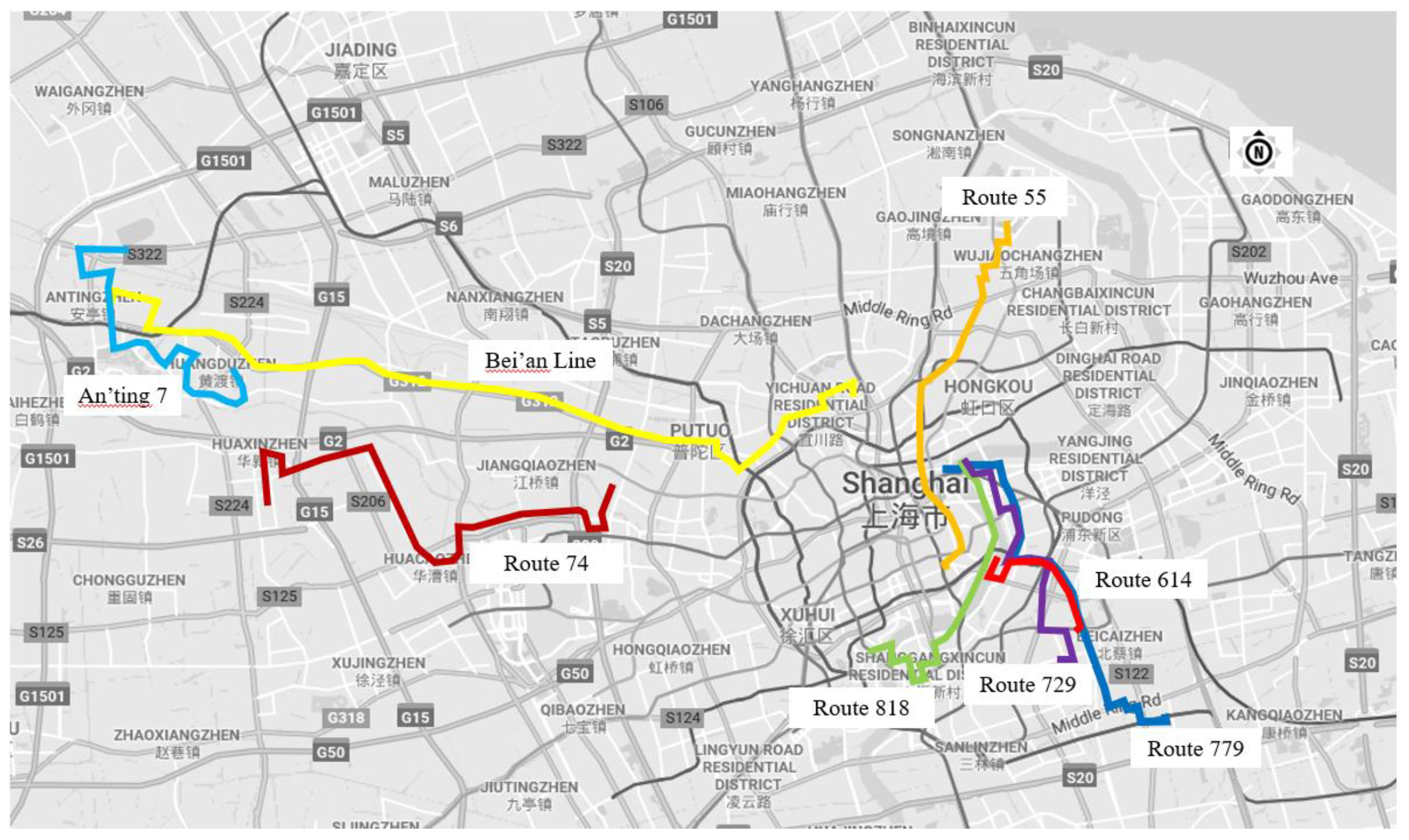
Considering the effects of route type and bus lane on bus emissions, eight bus routes were selected for data preparation covering different road levels and regions, as shown in Figure 1. Four bus routes (An’ting 7, Bei’an line, route 74, and route 55) are operated in the West of Shanghai, while the reminder four bus routes (route 818, route 729, route 614, and route 779) are operated in the East of Shanghai, reflecting the different regions on bus emissions.

Figure 1.
Bus routes selection for data collection.
Table 1 shows the details of each bus route, including route type, route length, number of bus stops, average distance between two adjacent bus stops (ADBS), proportion of bus lane length and average distance between two adjacent intersections (ADI). Taking the downtown line route 818 for example, the road length is about 12.4 km, the total number of bus stops is 18, the values of ADBS and ADI are 729 m and 430 m, and the percentage of bus lane length is 42.4%.

Table 1.
Details of each selected bus route for data preparation. Abbreviations: average distance between two adjacent bus stops (ADBS), average distance between two adjacent intersections (ADI).
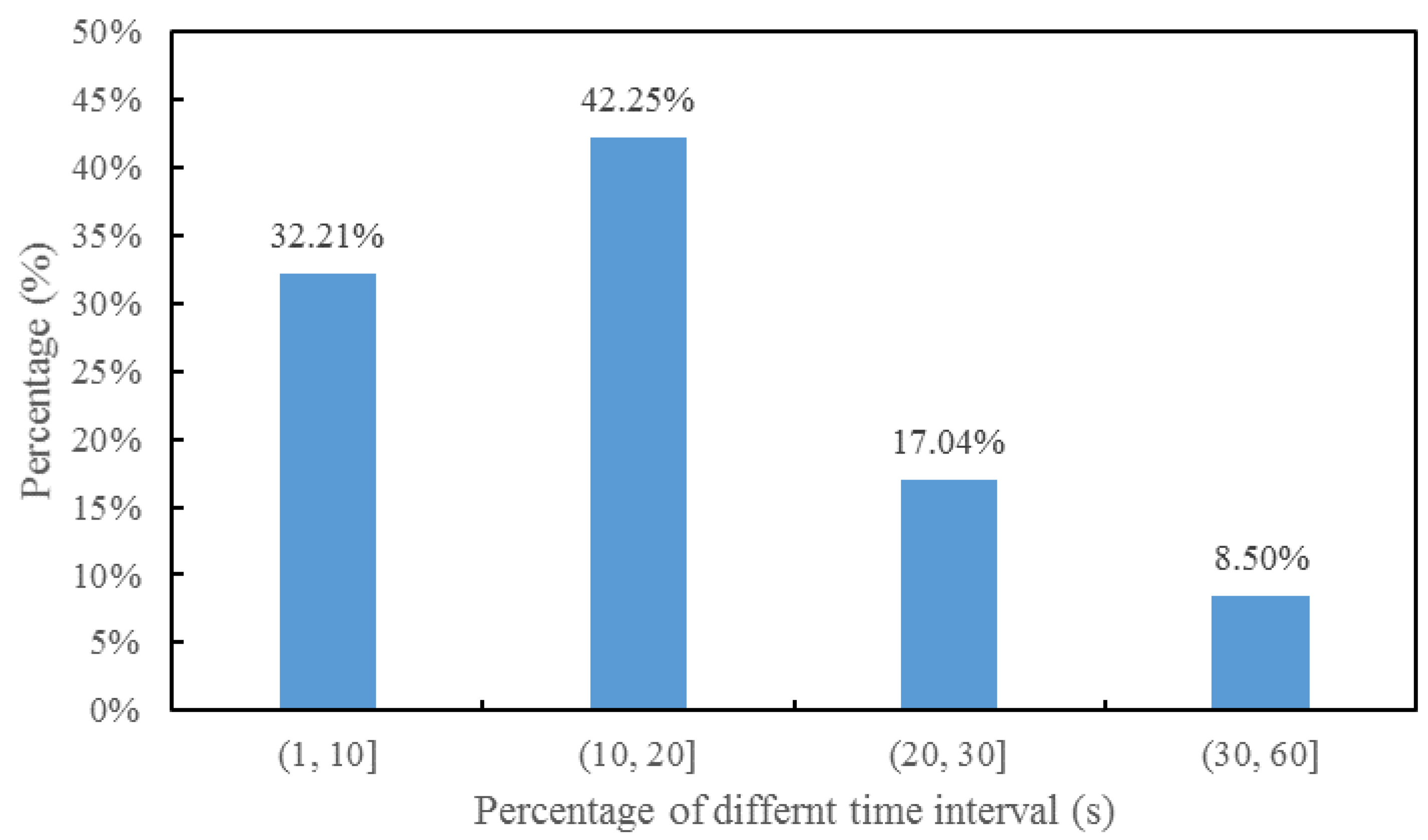
Each bus is equipped with GPS device. Data of bus position and speed are sent to the city’s traffic management center with a certain time interval. Sparse GPS data of forty-three buses are obtained from Shanghai’s traffic management center covering the eight bus routes described above. Figure 2 shows the distribution of time intervals for a certain bus sending its information to traffic center. We find that about 75% of GPS data are sent to traffic center with a time interval lower than 20 s, only 8.5% of data are sent with a time interval higher than 30 s.

Figure 2.
Percentage of different time intervals for a certain bus.
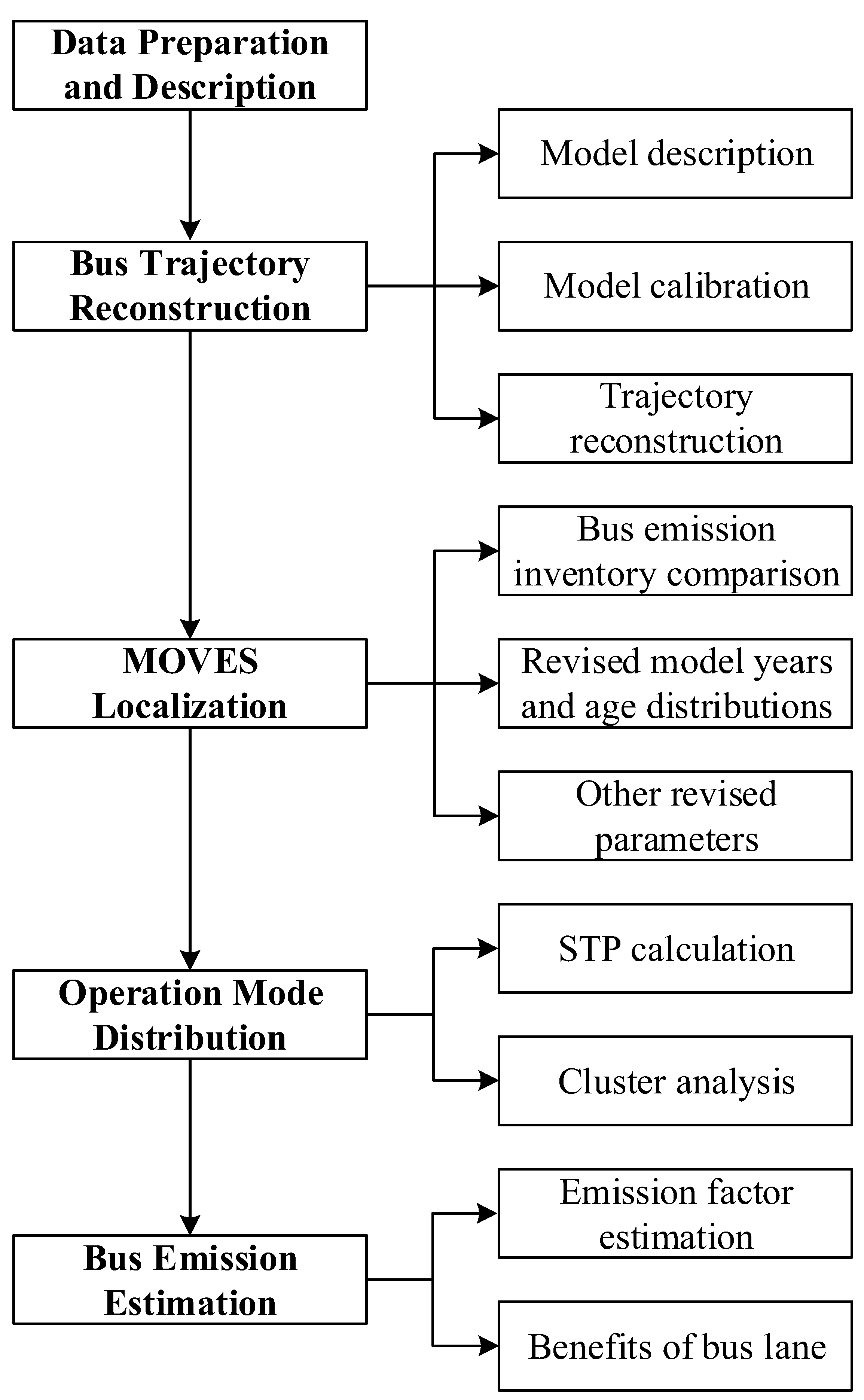
This study aims to evaluate urban bus emission characteristics based on localized MOVES using sparse GPS data in Shanghai, China. The overall analysis framework is shown in Figure 3. After data collection and preparation, bus trajectories can be reconstructed using modal activity-based model proposed by Shan et al. [15]. The framework of modal activity-based model is first introduced, followed by model calibration results for bus type using the collected second-by-second bus trajectory data. Then bus trajectories are reconstructed using sparse GPS data.

Figure 3.
Overall research framework of this study. STP: scaled tractive power.
Due to the shortage of local microscopic vehicle emissions model in China, MOVES should be localized to reflect local vehicle characteristics. The following three steps are conducted: (1) comparing bus emissions inventory between US and China to find the suitable bus emissions rates stored in MOVES database for buses in China; (2) revising model years and vehicle age distributions to reflect local bus emission standards; (3) localizing other parameters, such as fuel supply, meteorology and road types etc.
As the key input into MOVES, local link operation mode distributions are calculated based on the formula of scaled tractive power (STP) using the reconstructed bus second-by-second trajectories, which is introduced in Section 5. Then cluster analysis of K-means method is adopted to explore the characteristics of vehicle operation mode distributions under different traffic conditions. Finally, based on MOVES localization and local bus operation mode distributions, bus emission factors are estimated including hydrocarbon compounds (HC), carbon monoxide (CO), nitrogen oxide (NOx), and PM2.5 (fine particulate matter, particles with aerodynamic diameter less than 2.5 um). Benefits of bus lane on bus emission reductions are also analyzed.
3. Bus Trajectory Reconstruction Using Sparse GPS Data
3.1. Modal-Activity Based Model Description
Hao et al. [16] proposed the original modal activity-based model to reconstruct vehicle trajectory on arterial roads with a strong assumption, which is that the driving modes of a vehicle must evolve with a certain pattern, i.e., idle → acceleration → cruise → deceleration → idle →… periodically. Shan et al. [15] released such strong assumption, they assumed that there may exit an inflection speed during the time interval for a certain data pair, and modal transition only happens at the starting speed, ending speed and inflection speed. The framework of Shan’s revised modal activity-based model is descripted as follows:
3.1.1. Identifying Vehicle Dynamic State
There are four kernel matrixes to determine a vehicle dynamic state, named modal activity sequence (M), modal transition speed vector (V), travel time vector (T), and distance vector (X). For a certain sparse data pair, based on the starting speed (u1) and the ending speed (u2), we can determine the probability of a certain valid vehicle dynamic state {m, v, t, x}, using Equation (1).
where, is the time interval, is the total traveling distance during the time interval, and K is the length of M.
3.1.2. Reconstructing Vehicle Trajectory for Acceleration/Deceleration Mode
To a certain acceleration/deceleration mode, we know the starting speed (vi), ending speed (vi+1), time consumption (ti), and traveling distance (xi). Equations (2) and (3) can be used to estimate the second-by-second vehicle speed. We assume that the accelerate rate follows a linear acceleration mode, .
3.1.3. Considering the Speed Oscillation Effect of Cruising Mode
Speed oscillation effect of cruising mode should be integrated in vehicle trajectory reconstruction. Equation (4) is used to generate a vector A = , which follows a Gaussian distribution and satisfy the constraint ().
where, B = is ( − 1) independent normal random numbers following , e is a 1 × all-one matrix, and Q is the × ( − 1) orthonormal basis matrix.
3.1.4. Selecting the Best Vehicle Dynamic State
We select the best scenario {m*, v*, t*, x*} with the largest probability in a valid vehicle dynamic state, using Equation (5). Then, vehicle trajectory could be reconstructed.
3.2. Model Calibration for Bus Type
Shan et al. [15] conducted model calibration for LDVs on freeways and arterial roads. In this study, second-by-second vehicle trajectory data from two buses are collected for model calibration for bus type. Model calibration includes the following three aspects:
3.2.1. Driving Mode Segmentation
The kinematic parameter method with five parameters, (a1, a2, a3, a4, and a5) proposed by Shan et al. [15] is adopted to segment driving mode for ground truth. For an acceleration driving mode, the instantaneous accelerations should be greater than a1 m/s2, lasting for 3 s or longer, leading to a speed increment larger than a2 m/s. Similarly, for a deceleration driving mode, the absolute instantaneous decelerations are larger than a3 m/s2, lasting for 3 s or longer, with a speed decrease larger than a4 m/s. The remaining speed points are classified as cruising (speed larger than a5 m/s) or idling driving mode. Genetic algorithm is used to calibrate these five parameters. Equation (6) is the function of fitness.
where is the standard deviation of acceleration of any cruising mode; is the average acceleration of any cruising mode; is the weight for the objective of , with the value of 0.5 in this study; N is the total time of cruising mode, representing the average error of one data point.
The calibrated results of these five parameters are 0.11 m/s2, 0.63 m/s, 0.22 m/s2, 0.68 m/s, and 0.42 m/s. Compared with the calibration results of LDVs on arterial roads in Shan et al. [15], we find that the acceleration/deceleration intensities of bus type show much smaller than the intensities of LDVs because of the impact of bus stops.
3.2.2. Probability Estimation of Inflection Speed Point
Using the collected vehicle trajectory data, we generate the different time interval data pairs. We calculate the gap between the inflection speed and the average speed , donated as . The Gaussian Mixture Model (GMM) is used to estimate the probability of . The probability density function of is formulated as follows:
where, g is the index of Gaussian distributions; is the weighting factor associated with the gth Gaussian distribution () and . We set G = 2. Then maximum likelihood method is applied to calibrate the values of .
Expectation maximization algorithm is used to solve Equation (8). The parameters of GMM for different time intervals for urban bus on arterial roads are listed in Table 2.
Table 2.
Parameters for Gaussian Mixture Model (GMM) with the different time intervals for urban bus on arterial roads.
3.2.3. Distribution Parameters for Driving Modals
We assume the acceleration pace follows a Gaussian distribution (see Equation (9)). The distance that a vehicle travels under the acceleration/deceleration mode also follows another Gaussian distribution (Equation (10)),
where vs and ve are the instant speed at the start and end of the acceleration/deceleration modal respectively. Maximum likelihood estimation method is adopted to parameters calibration. Table 3 shows the calibration results of urban bus for acceleration and deceleration modals.
Table 3.
Parameters calibration of urban bus for acceleration and deceleration modals.
For speed oscillation effect of cruising modal, we assumed the accelerating rate of cruising modal followed a Gaussian distribution . The calibrated value of is 0.266 m/s2 for urban bus on arterial roads.
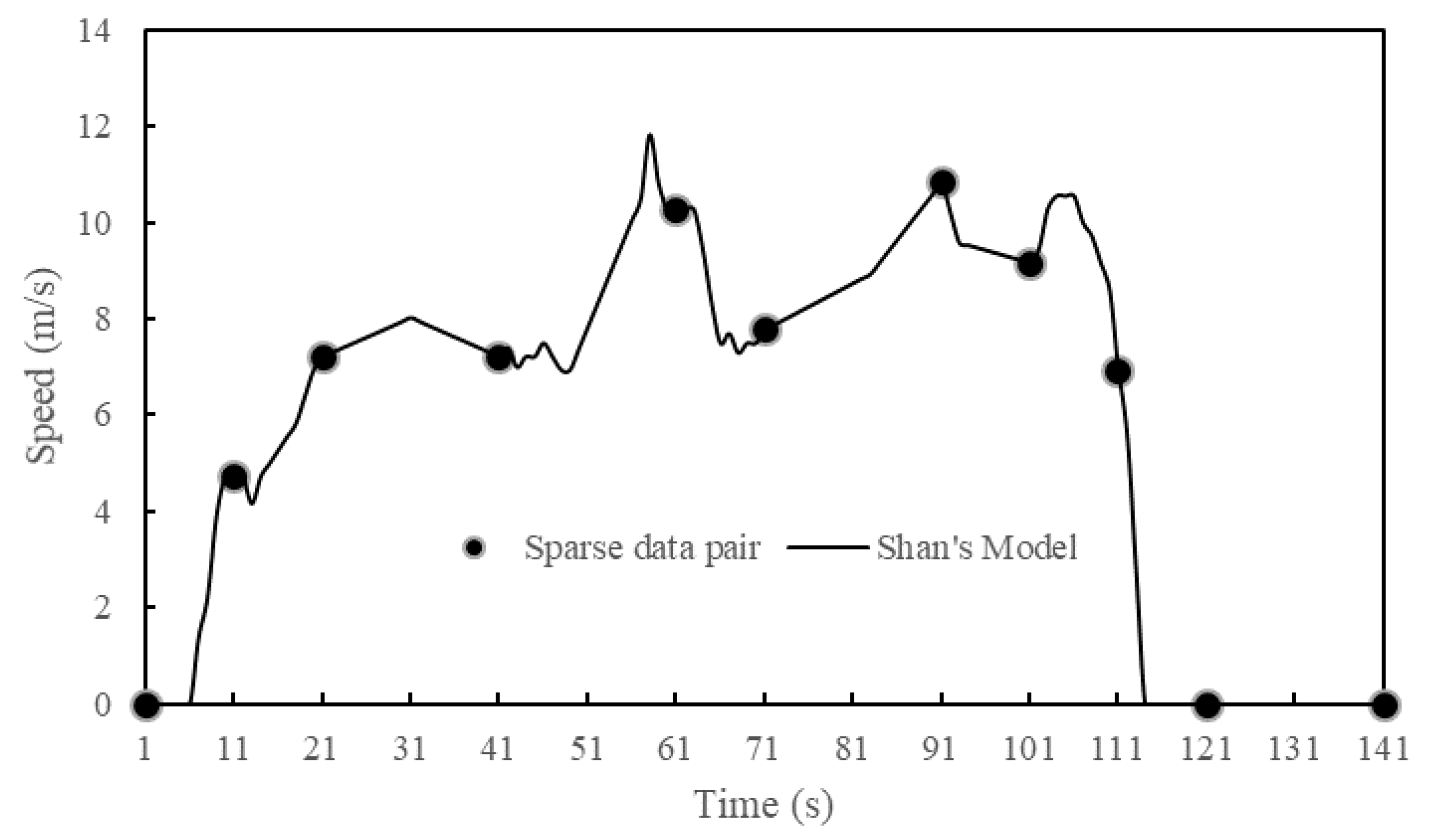
3.3. Trajectory Reconstruction Using Sparse GPS Data
Based on Shan’s model and calibration results of bus type, bus trajectories are reconstructed using sparse GPS data. Figure 4 shows the result of a certain bus speed–time trajectory reconstruction with a twenty-second time interval. Shan’s model shows good performance on bus trajectory reconstruction, with the consideration of real-world driving behavior, such as acceleration/deceleration intensity and speed oscillation effect of cruising modal.

Figure 4.
Results of a certain bus trajectory reconstruction.
4. MOVES Localization
4.1. Bus Emissions Inventory Comparison
As a type of HDV, conventional diesel buses’ emission characteristics are examined in this study. China’s vehicle emissions standard for HDVs was proposed in 2001, releasing the emissions limit values of China I phase and China II phase. Then, HDVs’ emission standard was revised in 2005. Time periods and vehicle emissions limits for China III phase, China IV phase, and China V phase have been released through the revised HDVs’ emission standard.
A European steady state cycle measurement and a European load response test were conducted to test the exhaust pollutants from compression ignition and gas fueled positive ignition engines of HDVs. Note that the unit of standard emission factors of HDVs is g/kw·h, rather than g/km.
Table 4 shows the comparison of emission limits for diesel fueled HDVs between US and China. For HC and CO emissions limits, there is no difference between China and US. For NOx, the years of emission limits for HDVs in the US are ahead of the years of emission limits in China. For example, China I phase of NOx for HDVs starts in 2001, while US starts in 1990, demonstrating the necessity of revising vehicle fleet age distribution. The related years for PM emission in the US compared with five phases in China are 1990, 1994, 1994, 2007, and 2007.
Table 4.
Emissions limits for diesel fueled heavy-duty vehicles (HDVs) comparison between the US and China (g/kw·h).
4.2. Bus Age Distribution Revision
Due to the differences of emissions limits standards between China and the US, it is necessary to revise bus age distribution to reflect the actual vehicle fleet characteristics in Shanghai, China. As a kind of commercial vehicle, the lifetime of a bus in Shanghai, China is eight years. Bus sparse GPS data were collected in May 2013. Thus, There are only three bus emission standard phases during that period, including China II phase, China III phase, and China IV phase. Figure 5a illustrates the original bus age distribution of a bus fleet. We find that vehicle average age is 5.5 years in Shanghai, China. The proportion of buses which are eight years old is 20.3%, larger than the other age categories. Note that the proportion of new buses operated in 2013 is only 5.5%.
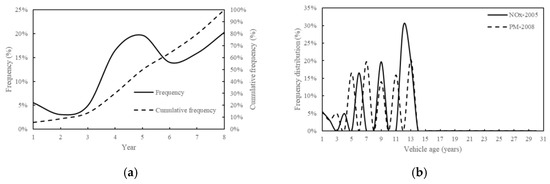
Figure 5.
(a) original bus age distribution; (b) revised bus age distribution.
For HC and CO emissions estimation, there is no revision on model years and bus age distributions. For NOx, buses operated in 2013 (compliant with China IV phase emission standard) is equivalent to the US buses operated in 2005. Thus, model year for NOx estimation should be revised to 2005, and bus age distribution should be revised to match the actual situation in Shanghai, China, as shown in Figure 5b. Similarly, the model year for PM estimation should be revised to 2008. Furthermore, the revised bus age distributions are different for the different vehicle emissions due to the different control processes in China and the US (see Figure 5b).
4.3. Other Localized Parameters
In addition to the revised model years and bus age distributions, other inputs required by MOVES, including fuel supply, vehicle/road type selection, and meteorological information, also need to be localized.
Fuel quality show a significant impact on vehicle emissions [17]. The limited sulfur level for conventional diesel buses in Shanghai, China is 50%. Thus, we select the MOVES fuel supply with an ID number of 26010 (sulfur level is 44%, the one most close to Shanghai’s level). As to vehicle type, the source type in MOVES is different to the highway performance monitoring system vehicle class. We select type ID 42 transit bus as the vehicle type in this study. Road type is set to be “urban unrestricted road”. Since temperature and humidity have significant impacts on vehicle emissions, we set the normal temperature to 25 °C (77 °F) and the humidity to 70% with consideration of the local meteorological conditions in Shanghai, China.
More importantly, local link vehicle operation mode distributions were calculated as the key input in MOVES, which will be presented in the next section. The length of each link was calculated by sparse GPS data and validated against Baidu Maps.
5. Bus Operation Mode Distribution and Emission Estimation
5.1. Local Link Operation Mode Distribution Calculation
As for HDVs, STP is used in MOVES to represent HDV power output (see Equation (11)). Table 5 shows the division principle of vehicle operation mode with 23 categories. Vehicle operation mode distribution describes the fractions of time consumed for each of the 23 categories,
where, v is vehicle instantaneous speed (m/s), a is vehicle acceleration (m/s2), g is gravity acceleration (m/s2), reflects road grade, m is the total mass of a bus with the number of 16 in this study, and is the fixed mass factor with the number of 17.1 in MOVES. A, B, and C are the road load factors, with the unit of kw·s/m, kw·s2/m2 and kw·s3/m3.
Table 5.
Vehicle operation mode division principle in MOtor Vehicle Emission Simulator (MOVES).
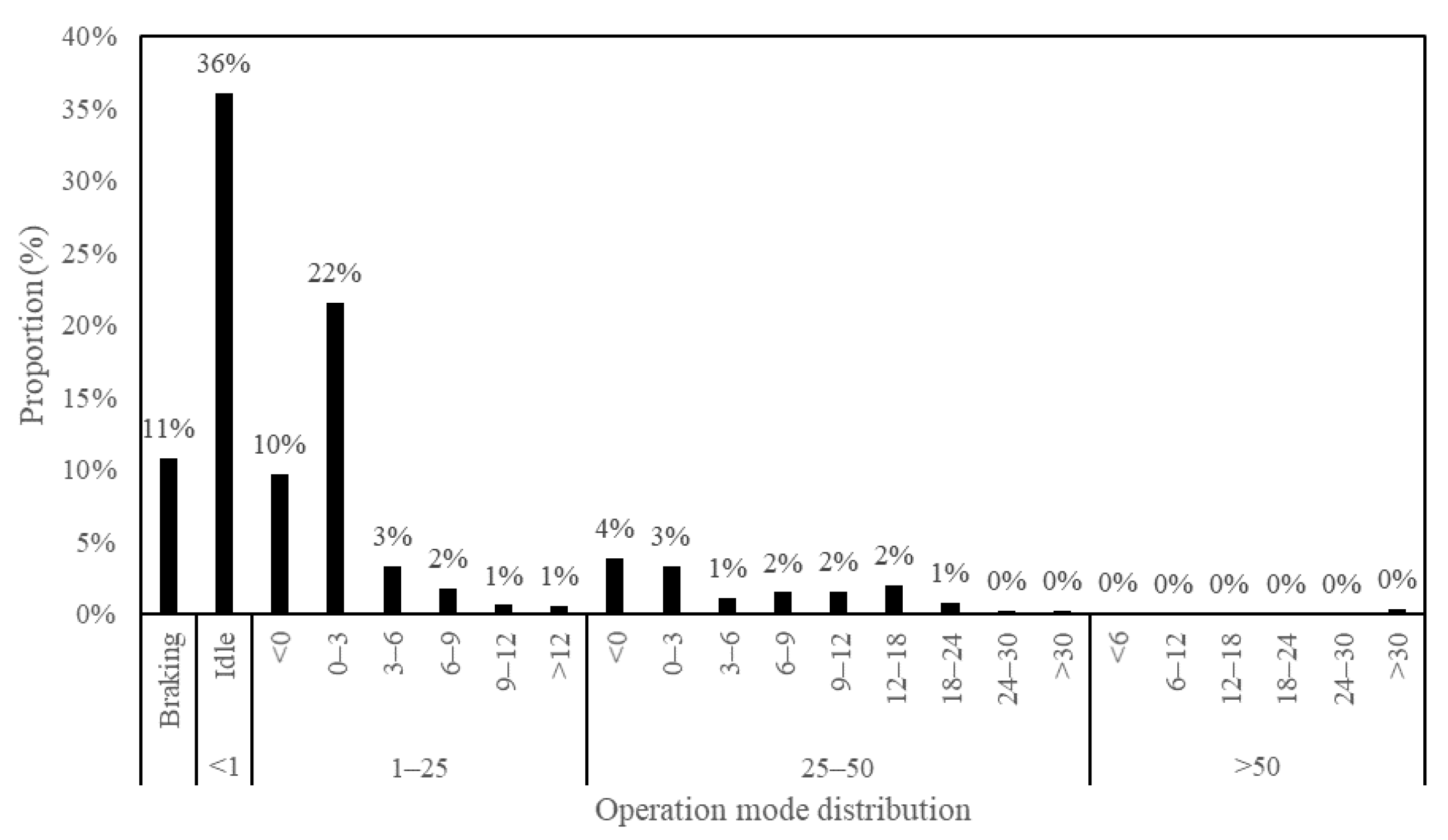
Figure 6 shows the operation mode distribution of a certain bus for a link. The average speed of this bus is about 14.7 km/h, and the road length of this link is about 1.2 km. Due to the influence of bus stops and signal intersections, this bus accelerates and decelerates frequently, resulting in the highest proportion (36%) of idling driving mode. The second highest proportion of operation mode is Bin 12 at 22%, showing the long duration of bus operation at low speeds. Meanwhile, there is no operation mode for high speeds, such as vehicle traveling speed larger than 50 mph (or 80 km/h), due to the speed limits of buses.
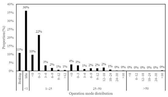
Figure 6.
Operation mode distribution for a certain bus with the average speed of 14.7 km/h.
5.2. Cluster Analysis of Bus Operation Mode Distributions
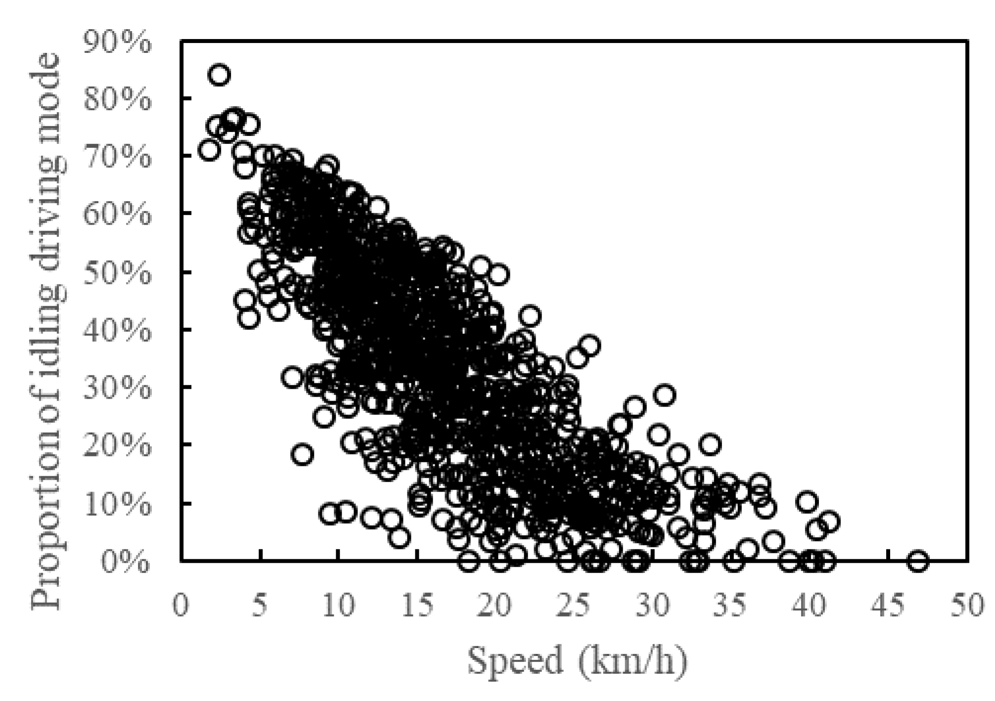
Vehicle operation mode distributions of 892 links were calculated from bus sparse GPS datasets. The average speed of these buses ranges from 1.5 km/h to 47 km/h, covering different traffic conditions. Road length varies from 1 km to 3 km. Figure 7 shows the relationship between traveling speed and the proportion of idling operation mode (recorded as Bin 1 in Table 5).

Figure 7.
Relationship between average traveling speed and proportion of idling operation mode.
As shown in Figure 7, with the increase of vehicle traveling speed, the proportion of idling operation mode (Bin 1) shows a decreasing trend. When the traveling speed is less than 5 km/h, the proportion of Bin 1 is larger than 70%; in contrast, when the traveling speed is higher than 40 km/h, the proportion of Bin 1 is lower than 10%. Meanwhile, proportions of Bin 1 show difference even at the same average speed due to the different driving patterns, resulting in different emission factors as discussed in next section.
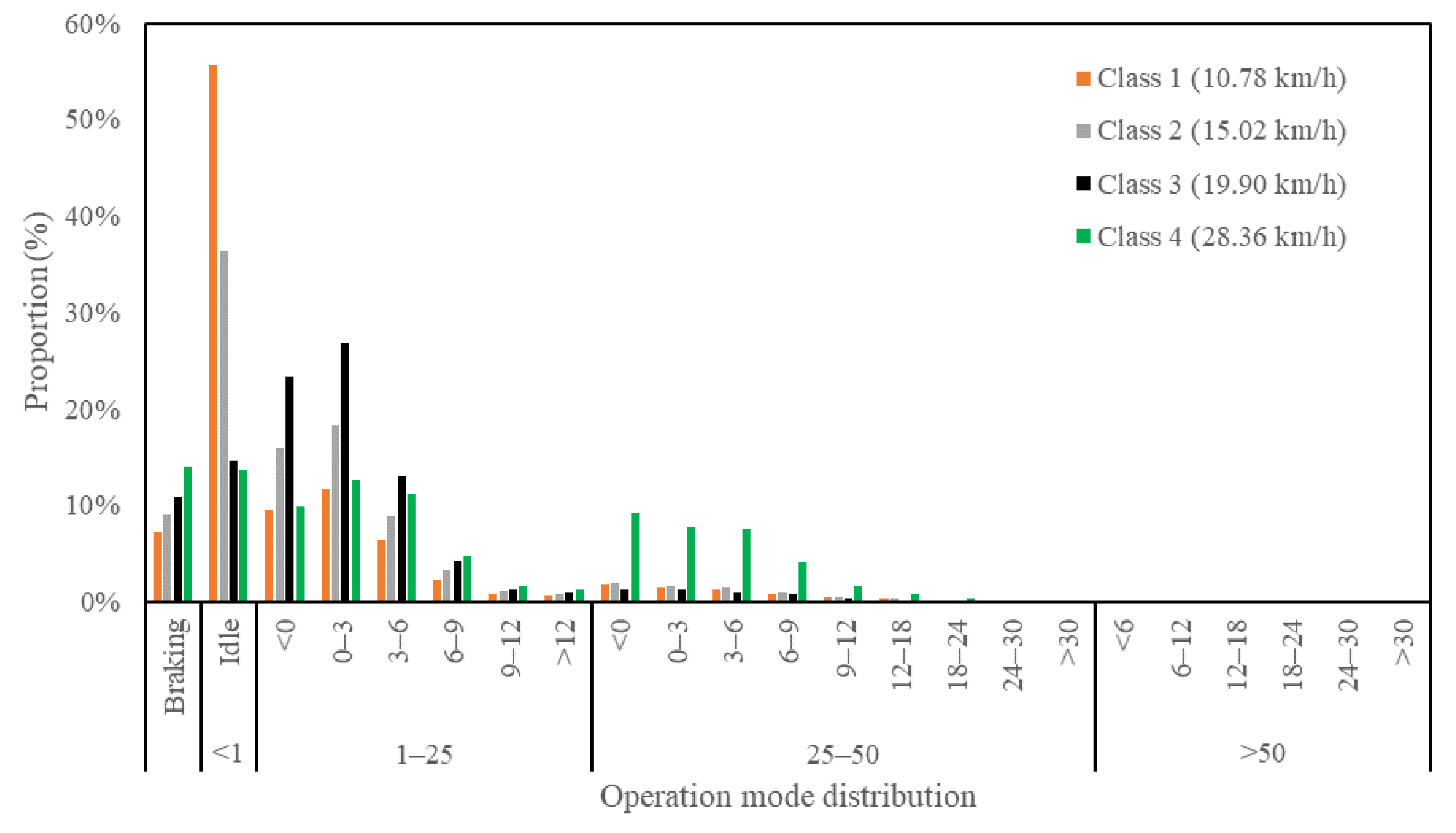
The K-means cluster analysis method is adopted to explore the characteristics of vehicle operation mode distributions considering different traffic conditions, implemented in Matlab [18]. Table 6 shows the classified criteria for road traffic performance level of service (LOS) in China [19]. For example, as for the major roads, there are four key speeds to divide different road traffic performance levels. The values are 40 km/h, 30 km/h, 20 km/h, and 15 km/h, respectively. Thus, in our study, we set K equal to 4. Figure 8 shows the four typical vehicle operation mode distributions. Average speed of each typical vehicle operation mode distribution is also calculated.
Table 6.
Classified criteria for road traffic performance levels. LOS: level of service.

Figure 8.
Cluster analysis result on typical vehicle operation mode distributions.
As exhibited in Figure 8, class 1 shows the largest proportion of idling operation mode (55.6%) with the average speed of 10.78 km/h; the average traveling speed of classes 2 and 3 are 15.02 km/h and 19.90 km/h, respectively. Class 4 shows the lowest proportion of idling operation mode (13.6%) with the average speed of 28.36 km/h. For class 4, when the speed is higher than 28 km/h, there are some high operation modes with proportions greater than 5%, such as Bin 21, Bin 22, and Bin 23.
5.3. Bus Emission Estimation
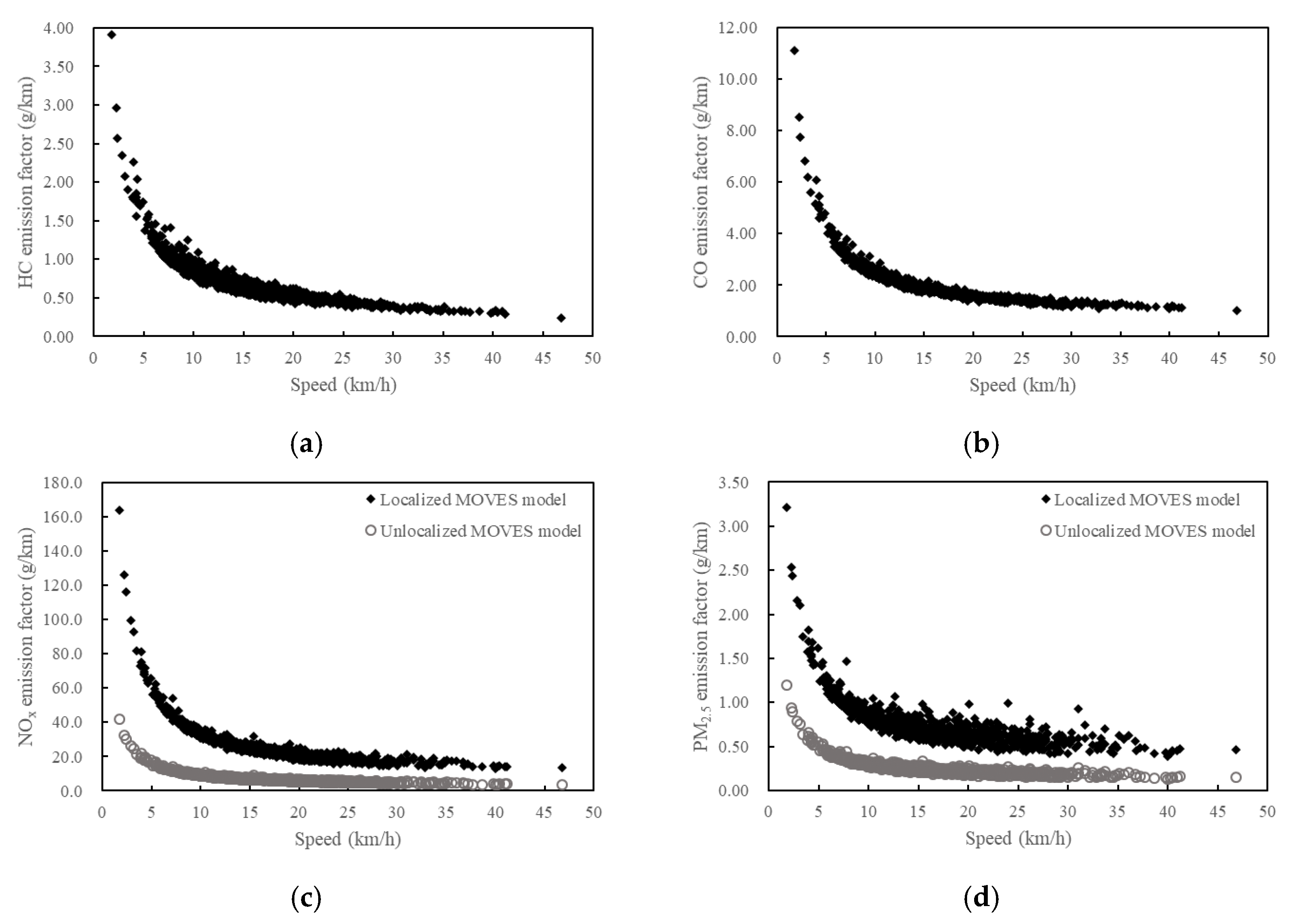
Based on MOVES localization and calculated bus operation mode distributions, bus emission factors were estimated, as shown in Figure 9. Overall, with the increase of vehicle traveling speed, bus emission factors first showed a rapid decrease and then slowly declining trend, towards some minimum values. The emission factors of HC, CO, NOX, and PM2.5 varied from 0.25 g/km to 3.92 g/km, 1.03 g/km to 11.12 g/km, 12.86 g/km to 163.88 g/km, and 0.38 g/km to 3.22 g/km, respectively. Compared to LDVs, buses show higher NOx and PM2.5 emission factors, due to their fuel type and higher vehicle weight.
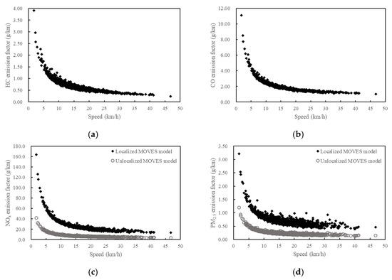
Figure 9.
(a) bus HC emission factor estimation; (b) bus CO emission factor estimation; (c) bus NOx emission factor estimation; (d) bus PM2.5 emission factor estimation. Abbreviations: hydrocarbon compounds (HC), carbon monoxide (CO), nitrogen oxide (NOx), and PM2.5 (fine particulate matter).
For comparison, NOx and PM2.5 emission factors are also estimated using original MOVES. Results show that NOx emission factor estimated from localized MOVES is about 3.6 times greater than estimation factor estimated from the original MOVES. For PM2.5, the emission factor estimated by localized MOVES is about 2.9 times larger than the that from the original MOVES. The significant differences in emission estimation between localized MOVES and original MOVES highlights the necessity of MOVES localization.
5.4. Benefits of Bus Lane on Bus Emission Reductions
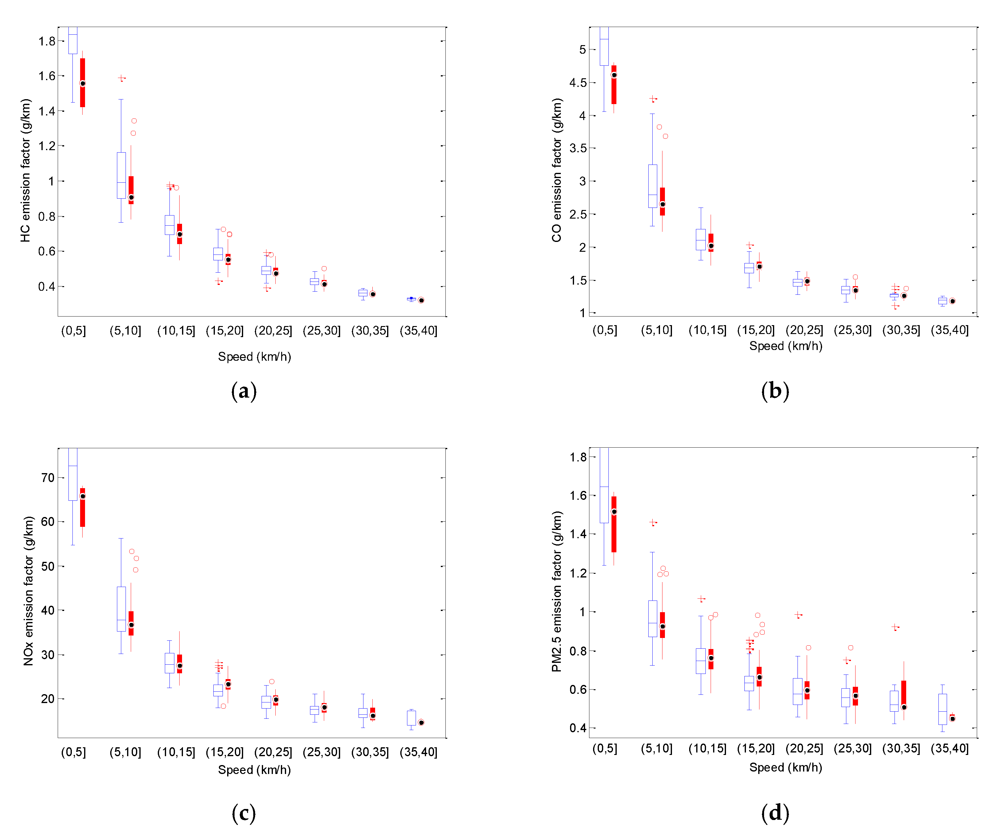
Figure 10 shows the boxplots of emissions factors with or without bus lane segmented by different traveling speed. The boxplots show the range, upper/lower quartiles, and median observed values, with statistical outliers as crosses or circles. The red-filled rectangles represent emission factors for buses operating on bus lane, while the emission factors for buses on non-bus lane are denoted by the blue rectangles.

Figure 10.
(a) bus HC emission factor estimation; (b) bus CO emission factor estimation; (c) bus NOx emission factor estimation; (d) bus PM2.5 emission factor estimation. Noted that red-filled rectangle shows the estimation results with bus lane, the hollow rectangle shows the estimation results without bus lane.
Figure 10 indicates that under serious traffic congestion (traveling speed lower than 10 km/h), on average, a bus operating on bus lane emits less pollutants than its counterpart on non-bus lane. The emission reduction benefits of bus lanes can be explained by the fact that buses accelerate or decelerate more frequently when mixing with private cars under traffic congestion period. However, when the traveling speed is higher than 10 km/h, bus lane does not show a significant effect on reducing bus emissions.
6. Conclusions
This paper aimed to explore the characteristics of bus operation mode distributions and emission factors based on localized MOVES using sparse GPS data in Shanghai, China. Eight bus routes with forty-three buses were selected for data preparation covering different road levels and regions. A research framework was then proposed, including bus trajectory reconstruction, MOVES localization, operation mode distribution analysis, and emission factors estimation. For bus trajectory reconstruction, the modal activity-based model was first introduced, followed by model calibration for urban bus and bus trajectory reconstruction using sparse GPS data. The modal activity-based model showed better performance than the linear interpolation model, with consideration of the real-world driving behaviors, such as acceleration intensity and speed oscillation effect of cruising modal.
As to MOVES localization, bus emission inventories between China and the US were compared for different emission limits to match the model year. Age distribution of bus fleets and other parameters were also revised to reflect local features in Shanghai, China. Based on the reconstructed bus trajectories, vehicle operation mode distributions were analyzed. Results reveal that with the increase in vehicle traveling speed, the proportion of idling operation mode showed a decreasing trend. Four typical operation mode distributions were identified using K-means cluster analysis. The average speeds of these distributions were 10.78 km/h, 15.02 km/h, 19.90 km/h, and 28.36 km/h, respectively.
Finally, bus emission factors were estimated using localized MOVES and calculated bus operation mode distributions. Bus emission reduction benefits of bus lanes were also analyzed. Results showed that with the increase in traveling speed, vehicle emission factors first showed a rapid decreasing and then a slowly declining trend, towards some minimum values. Under traffic congestion with traveling speed less than 10 km/h, the emission factors of a bus operating on bus lane were lower than that from a vehicle operating on non-bus lane. In contrast, when the traveling speed was greater than 10 km/h, there was no significant difference in emission factors between bus lanes and non-bus lanes. The findings of this study will be useful for understanding the relationship between traffic conditions and bus emission characteristics.
Note that this study was conducted mainly based on MOVES, and a validation of the emission estimation performances using real-world PEMS data is needed for future work. The MOVES localization method proposed in this study was a little complex, leading to the necessity of proposing a new localization method to decrease complexity. For example, some average values can be regarded as the input of localization to estimate bus emissions instead of age distribution revision. Furthermore, other vehicle types such as LDVs and heady-duty trucks should also be evaluated in emission estimation. Lastly, the authors note the limitation of the vehicle trajectory reconstruction model which fails to consider many other factors, such as two or more inflection speeds and GPS position errors, though model validation indicates its good performance.
Author Contributions
X.S. and X.C. conceived and designed the paper, X.S., X.C., W.J. and J.Y. collected and analyzed data and wrote the paper.
Funding
This research is funded by the Fundamental Research Funds for the Central Universities (No. 2018B08014) and by the National Science Foundation of China (No. 51608171).
Acknowledgments
I am extremely grateful to Shanghai Municipality Transport Information Centre (SMTIC) for data sharing and data processing.
Conflicts of Interest
The authors declare no conflict of interest.
References
- Farrell, L.; Pelaez, E.R.M.; Comerford, G.; Frazier, R.; Goff, M.; Ahmed, S.; Park, H.J.; Weeks, A.J. MOVES Project Level Traffic and Air Quality Analyses—Collaborative Approach. In TRB 94th Annual Meeting Compendium of Papers; Paper #15-1869; CD-ROM, Transportation Research Board of the National Academies: Washington, DC, USA, 2015. [Google Scholar]
- Methodology for the UK’s Road Transport Emissions Inventory. Available online: https://uk-air.defra.gov.uk/assets/documents/reports/cat07/1804121004_Road_transport_emissions_methodology_report_2018_v1.1.pdf (accessed on 13 March 2018).
- Edwardes, W.; Rakha, H. Virginia Tech Comprehensive Power-Based Fuel Consumption Model: Diesel and Hybrid Buses. J. Transp. Res. Board 2014, 2428, 1–9. [Google Scholar] [CrossRef]
- Edwardes, W.; Rakha, H. Modeling Diesel and Hybrid Bus Fuel Consumption Using VT-CPFM: Model Enhancements and Calibration Issues. In TRB 94th Annual Meeting Compendium of Papers; Paper #15-2198; CD-ROM, Transportation Research Board of the National Academies: Washington, DC, USA, 2015. [Google Scholar]
- Alam, A.; Hatzopoulou, M. Investigating the Isolated and Combined Effects of Congestion, Roadway Grade, Passenger Load, and Alternative Fuels on Transit Bus Emissions. Transp. Res. Part D 2014, 29, 12–21. [Google Scholar] [CrossRef]
- Alam, A.; Xu, J.; Hatzopoulou, M. An Analysis of Instantaneous Speed Distributions and Emissions for Transit Buses across an Urban Network. In TRB 94th Annual Meeting Compendium of Papers; Paper #15-2941; CD-ROM, Transportation Research Board of the National Academies: Washington, DC, USA, 2015. [Google Scholar]
- Chen, X.; Shan, X.; Ye, J.; Yi, F.; Wang, Y. Evaluating the Effects of Traffic Congestion and Passenger Load on Feeder Bus Fuel and Emissions Compared with Passenger Car. Transp. Res. Procedia 2017, 25, 616–626. [Google Scholar] [CrossRef]
- Jia, W.; Chen, X.; Shan, X. Modeling Urban Bus Fuel Consumption in Shanghai, China, Based on Localized MOVES. Transp. Res. Rec. 2018, 2484, 149–158. [Google Scholar] [CrossRef]
- Wang Chao Ye, Z.; Yu, Y.; Gong, W. Estimation of bus emission models for different fuel types of buses under real conditions. Sci. Total Environ. 2018, 640–641, 965–972. [Google Scholar] [CrossRef] [PubMed]
- Yu, Q.; Li, T. Evaluation of bus emissions generated near bus stops. Atmos. Environ. 2014, 85, 195–203. [Google Scholar] [CrossRef]
- Yu, Q.; Li, T.; Li, H. Improving urban bus emission and fuel consumption modeling by incorporating passenger load factor for real world driving. Appl. Energy 2016, 161, 101–111. [Google Scholar] [CrossRef]
- Li, F.; Zhuang, J.; Cheng, X.; Li, M.; Wang, J.; Yan, Z. Investigation and prediction of heavy-duty diesel passenger bus emissions in Hainan using a COPERT model. Atmosphere 2019, 10, 106. [Google Scholar] [CrossRef]
- Liu, H.; Chen, X.; Wang, Y.; Han, S. Vehicle Emission and Near-Road Air Quality Modeling for Shanghai, China Based on Global Positioning System Data from Taxis and Revised MOVES Emission Inventory. J. Transp. Res. Board 2013, 2340, 38–48. [Google Scholar] [CrossRef]
- Perugu, H. Emission modelling of light-duty vehicles in India using the revamped VSP-based MOVES model: The case study of Hyderabad. Transp. Res. Part D 2018, 68, 150–163. [Google Scholar] [CrossRef]
- Shan, X.; Hao, P.; Chen, X.; Boriboonsomsin, K.; Wu, G.; Barth, M. Vehicle energy/emissions estimation based on vehicle trajectory reconstruction using sparse mobile sensor data. IEEE Trans. Intell. Transp. Syst. 2019, 20, 716–726. [Google Scholar] [CrossRef]
- Hao, P.; Boriboonsomsin, K.; Wu, G.; Barth, M. Modal activity-based stochastic model for estimating vehicle trajectories from sparse mobile sensor data. IEEE Trans. Intell. Transp. Syst. 2017, 18, 701–711. [Google Scholar] [CrossRef]
- Nelson, F.P.; Tibbett, R.A.; Day, J.S. Effects of vehicle type and fuel equality on real world toxic emissions from diesel vehicles. Atmos. Environ. 2008, 42, 5291–5303. [Google Scholar] [CrossRef]
- Azimi, M.; Zhang, Y. Categorizing freeway flow conditions by using clustering methods. J. Transp. Res. Board 2010, 2173, 105–114. [Google Scholar] [CrossRef]
- Urban Road Traffic Performance Index, 2011. Available online: http://jtw.beijing.gov.cn/xxgk/flfg/r764/201111/P020141111625117643012.pdf (accessed on 28 April 2011).

© 2019 by the authors. Licensee MDPI, Basel, Switzerland. This article is an open access article distributed under the terms and conditions of the Creative Commons Attribution (CC BY) license (http://creativecommons.org/licenses/by/4.0/).