Article

Estimation of Soil Respiration by Its Driving Factors Based on Multi-Source Data in a Sub-Alpine Meadow in North China

1
State Key Laboratory of Water Environment Simulation, School of Environment, Beijing Normal University, Beijing 100875, China
2
Institute of Loess Plateau, Shanxi University, Taiyuan 030006, China
3
Institute for Energy, Environment and Sustainable Communities, University of Regina, 120, 2 Research Drive, Regina, SK S4S 7H9, Canada
4
Beijing Engineering Research Center for Watershed Environmental Restoration & Integrated Ecological Regulation, School of Environment, Beijing Normal University, Beijing 100875, China
*
Authors to whom correspondence should be addressed.
Sustainability 2019, 11(12), 3274; https://doi.org/10.3390/su11123274
Submission received: 2 May 2019 / Revised: 1 June 2019 / Accepted: 1 June 2019 / Published: 13 June 2019
(This article belongs to the Section Environmental Sustainability and Applications)

Abstract

:
Soil respiration (Rs) in high-altitude areas are normally sensitive to varying climatic conditions. The objective of this research was mainly to explore temporal variations in Rs rates and the corresponding controlling factors for the establishment of appropriate fitting models in a sub-alpine meadow of north China. The data was obtained through field measuring and extraction of the Moderate Resolution Imaging Spectroradiometer (MODIS) in the geographical unit of the study site over the period of 2007 to 2015. The main results were as follows: (1) seasonal variations in Rs rates, soil temperature (Ts), land surface temperature (LST), and normalized difference vegetation index (NDVI) all produced symmetrical bell type patterns, while soil moisture (Ms) showed a fluctuating pattern, (2) a Ts-exponential model could greatly capture seasonal variations of Rs rates in the study site, reflecting the role of temperature as a dominant driving factor in determining Rs temporal variations in alpine meadow areas, (3) there was no significant difference between the performing indicators evaluating the proposed Ts-exponential model and the LST-exponential model. This indicated great potential for applying remote sensing products to estimate seasonal Rs rates and 4) seasonal variations in Rs rates towards temperature sensitivity (Q10) showed a concave curve and dramatically decreased as the temperature increased from −1 to 11 °C. Overall, the results indicated that attention to significant effects of climatic conditions on Rs, particularly in areas of low temperature, should be warranted. Also, applicability of remote sensing products for estimating Rs was reflected and demonstrated.

1. Introduction

In the past decades, concerns over the global carbon cycle are increasingly high due to its close relationships with global warming [1,2]. Increasing concentration of CO2 in the atmosphere is believed as the primary factor for the generation of greenhouse effects [3]. Moreover, the exchange of CO2 between the atmosphere and soil results in certain feedback to climatic change [4].
Soil CO2 efflux, hereafter referred to as soil respiration (Rs), is the second largest terrestrial carbon efflux and therefore considered to be one of the most significant components of the global carbon balance [5]. Raich and Potter [6] estimated that about 50–77 Pg C yr−1 of CO2 was released from the soil to the atmosphere, accounting for approximately 60%–90% of the ecosystem respiration, 40%–60% of the total primary productivity [7], and almost 10 times the amount of CO2 emitted by industrial combustion (5 Pg C yr−1) [8,9]. Moreover, the value of the “missing carbon sink” has increased, making it essential to study the response of Rs to climatic change. Additionally, quantitative observation of Rs is crucial to accurately estimating the carbon budget of a given area [2,10].
Soil respiration is a complex process of CO2 emission that involves autotrophic respiration and heterotrophic respiration, including the production of CO2 by plant roots, soil microbes, and soil fauna, and the subsequent emission of CO2 from soil to the atmosphere [11,12]. Thus, Rs is affected by a combination of environmental factors including temperature [13], soil water content [14], rainfall events [15,16], photosynthetic rate, physical and chemical characteristics of soil such as the dissolution of carbonates due to acidification in calcareous and limed acidic soils [11,17], soil biological properties [18], solar radiation, landform factors [3], and external disturbances [10]. Therefore, these biotic and abiotic elements could potentially provide effective parameter inputs for the modeling of Rs. Predicted dynamic models of Rs variation based on all related environmental factors affecting Rs are complex and often constructed according to several key factors controlling the main process. There is considerable evidence suggesting that Rs is closely related to variations in temperature in most ecological scenarios [5,19], as well as to the soil moisture in dry conditions [20], and gross primary photosynthesis (GPP) or vegetation indexes [21] in ecosystems with high coverage. Although the effects of these factors on Rs could not be separated directly, the relative significance of each variable to Rs differs in various ecosystems. The temperature sensitivity index of Rs (Q10) has often been used to describe the dependence of Rs on temperature; however, it is actually not constant at temporal or spatial scales. Rather, its value varies under different temperature conditions [2], especially at lower temperatures. Understanding the variation characteristics of Q10 is a key step in investigation of Rs characteristics that contributes to the rational estimation of regional carbon budgets.
An infrared gas dynamic analysis system is a reliable and convenient field soil carbon dioxide flux observation method within higher measuring accuracy than that of the static method. However, the observed results can only represent the carbon flux characteristics of a specific ecosystem in the particular environment, and it can not be directly applied to other regions. Also, long-time series quantification of Rs measured in situ remains challenging because of the need to conduct great amounts of field work and the uncertainties regarding different ecological scenarios. Increasing the sample size under the background of global climatic change is critical to accurately investigating the dynamic balance of the carbon cycle. Remote sensing is the only feasible means for large-scale continuous and quantitative observation of ecological indicators at present. It is a low-cost and convenient method of acquiring land surface parameters indirectly, which compound the mixed effects of plants and soil. This technique has been proven to be valid for the estimation of surface parameters (land surface temperature, soil water content, and surface reflectivity), but is less applicable to underground biochemical processes such as Rs [22,23]. Some researchers have recently used more accessible land surface parameters to build spatial [5] or temporal variation models of Rs to predict Rs based on empirical models and provide data supporting the carbon budget on a large scale. The application of remote sensing to studies of Rs based on long-term observations is not easy and has seldom been conducted. Therefore, taking the combination of remote sensing technology and ecology process as the breakthrough point and integrating multi-source data containing in situ measured data and spatial data products to study soil respiration along long time series is not only the demand for the development of remote sensing application, but also an effective way to solve the scale expansion of field observing.
As the second largest geographic unit in China, accounting for 70% of the world’s loess distribution and the largest loess accumulation area in the world, the Loess Plateau region has formed its own unique climate and topography, within the characteristics of high altitude distribution, is also faced with a lot of ecological function decline such as soil erosion, vegetation destruction caused by human activities, and climatic change. The terrestrial carbon cycle in the Loess Plateau is an important component of the global carbon balance.
Sub-alpine meadows are widely distributed in China, which are dominated by perennial herbs. As an important type of grassland ecosystem, ecological investigations of sub-alpine meadows have received the attention of researchers because their ecological functions are far greater than their economic values. In the present study, a typical mountain meadow in the Loess Plateau, which was one of only four meadows in Shanxi province, was investigated. The carbon balance in this high-altitude distributed ecosystem is extremely sensitive to climatic change; therefore, the temporal characteristics of the carbon cycle were investigated to provide basic datasets with actual reference values. Furthermore, applying Moderate Resolution Imaging Spectroradiometer (MODIS) data to the temporal variation model of in situ measured Rs will verify the science significance and feasibility of estimating Rs using remote sensing data.
The study was conducted to explore the temporal dynamics in Rs as well as its connections to temperature, soil moisture and vegetation index in a sub-alpine meadow in north China based on field measuring data and spatial data products. Thereafter the dynamic response model of seasonal variations in Rs could be formulated by its driving primary factors based on multi-source data, further quantitively examining the dominant role of temperature in soil respiration in the sub-alpine meadow zone and the potential applicability of spatial data products to estimate Rs. The hypotheses of this study were: (1) seasonal variations in Rs would be effectively estimated by its primary driving factors, (2) Rs was most sensitive to temperature variations in study area thus temperature would act as a key role in estimating seasonal variations in Rs in the sub-alpine meadow zone, and (3) MODIS products would be reliable indicators for the quantitative estimation of Rs in a certain statistical sense.

2. Materials and Methods

2.1. Overview of the Studying Site

A long-term study was conducted in Pangquangou National Natural Reserve (37°47′45″–37°55′50″ N, 111°22′33″–111°32′22″ E; 10,443 hm2) (Figure 1) in Shanxi Province, which is a rare green field on the Loess Plateau. The study area is located in the warm temperate continental monsoon climate zone, which is characterized by a cool and rainy summer and autumn and a cold, dry winter. A typical mountain climate has formed in the area because of the influence of the altitude and topography. According to the meteorological station, the average annual temperature is 3 °C–4 °C, with a monthly average temperature of 16.1 °C in July and –10.6 °C in January. The annual sunshine duration in the region is 2500–2800 h and the active accumulated temperature (≥10 °C) was 2100 °C. In addition, the annual precipitation is 600–800 mm, the majority of which occurs from June to September, the annual relative humility is 56%, and the frost-free period lasts for 92 days per year. The soil types in the region are cinnamon soil, mountain cinnamon soil, mountain leaching cinnamon soil, mountain brown soil, and sub-alpine meadow soil as the elevation goes from low to high [24,25]. From the foothill to the top of the mountain, the vegetation types are deciduous broad-leaved forest (1200–1750 m), mixed coniferous broad-leaved forest (1750–2200 m), cold-warm coniferous forest (2200–2600 m), and sub-alpine shrub meadow (2600–2720 m), in which sub-alpine meadow is the dominant type.
The experimental site was in the sub-alpine meadow zone (37°53′08.5″ N, 111°32′18″ E; 150 hm2) located at the top of the reserve, which is a typical mountain meadow in north China. The sub-alpine meadow was mainly composed of Kobresia bellardii and Carex lanceolata. The meadow grasses in the study area are luxuriant, with a grass layer height of 15–20 cm. In addition, the organic matter content in the upper soil layer is 10%–15%.

2.2. Experimental Procedures and Measurement of Rs and the Related Environmental Factors

Soil respiration (Rs) was measured once a month during April to November from August 2007 to November 2015. The diurnal variation of Rs was measured to eliminate the influence of diurnal range on seasonal variations. The Rs rate between 8:00 and 11:00 AM was almost equal to the daily average Rs in the study site [26]. Thus the measurements were conducted during 9:00 to 11:00 local time to minimize the influence of the daytime temperature fluctuations. Furthermore, all measurements were conducted on rain-free days.
Soil respiration was measured using a LI-COR 6400 portable photosynthesis system (LI-COR, Environmental Division, Lincoln, NE, USA) equipped with a LI-COR 6400-09 soil chamber with an area of 71.6 cm2 that calculated soil CO2 efflux in the chamber using optical absorption spectroscopy in the infrared range. Detailed information regarding the system is available elsewhere [19]. The spatial heterogeneity of Rs at the study site has been studied previously [25,26], which facilitated design of the sampling strategy and determination of the optimal sample size for the study site. At least 15 collars from PVC pipe were inserted 2–3 cm into the soil and the soil chamber was mounted on each collar at the time of observation. Three cycles of consecutive measurements on the collar were conducted to prevent any systematic errors, and the average Rs value was used for each collar. The plants were cut off inside the collars manually to avoid the effects of photosynthesis on Rs. To minimize the effects of soil disturbance during installation, all collars were installed at least 1 day before measurement. Hence, it was assumed that there was no disturbance caused by operation of the flux chamber or plant growth. The average soil CO2 efflux rate from all PVC collar measurements was recorded as the mean daily Rs at the measuring time in study site. The measuring frequency was once a month. The monthly Rs was computed by averaging all daily measured data in the corresponding month from August 2007 to November 2015 (n = 4 for April, 8 for May, 8 for June, 8 for July, 9 for August, 9 for September, 7 for October, and 5 for November) to get a representative monthly value. The frequency of the determination of related environmental factors were the same as for Rs.
The soil temperature (Ts) at depth of 5 cm was recorded using a thermocouple probe equipped with a portable photosynthesis system (LI-COR 6400) at locations near where Rs was measured. The soil moisture (Ms) was measured using soil samples collected from depths of 0–10 cm at the time of efflux measurement. Briefly, samples were returned to the laboratory and oven-dried at 105 °C until a constant mass was reached, and Ms was expressed as a percentage of dry soil mass.
MODIS eight-day surface reflectance products and eight-day land surface temperature (LST) products (MOD09A1, 0.5 km and MOD11A2, 1 km) in accordance with the in situ measuring time from NASA’s Earth Observing System Data and Information System (https://wist.echo.nasa.gov/api//) were downloaded. To match the measuring time of Rs, we obtained the LST and normalized difference vegetation index (NDVI) of the measuring day by linear interpolation of two consecutive eight-day spatial products. The pixel containing the study site was extracted based on the geo-location information (latitude and longitude). All the 15 or more sampling points in study site were in one pixel for retrieving the MODIS data based on the geo-location information. Each pixel contained the best possible observation coverage, low view angle, absence of clouds or cloud shadow and aerosol loading [5,23].
The land surface temperature (MOD11A2, 1 km) was derived by applying the generalized split-window algorithm [5,27]. The nighttime land surface temperature observed by MODIS onboard the Terra satellite is hereafter referred to as LST.
It is known that the most widely used normalized difference vegetation index (NDVI) is affected by soil reflectance in sparsely vegetated areas and saturates in cases of dense and multi-layered canopies [28]. The eight-day leaf area index (LAI) product (MOD15A2, 1 km) derived from surface characteristics [5] such as reflectance, land cover type, and other ancillary information, was mostly less than three in the geographic unit of study site, demonstrating that the most widely used NDVI could be a more suitable indicator of vegetation biophysical parameters than the enhanced vegetation index (EVI). The value of the normalized vegetation index (NDVI) was calculated from the two wavelength bands of surface reflectance using the following formula [29]:
NDVI = ρ Nir ρ R e d ρ Nir + ρ R e d
where ρNir and ρRed represent the reflectance for the near-infrared (MODIS band 2) and red (MODIS band 1) wavelength bands, respectively.

2.3. Modeling Strategy

All the monthly-measured data in each year was used for Rs model construction (n = 58) to explore the relationship between Rs and environmental factors. Also, all measured or downloaded data were verified for assumptions of normality and variance homogeneity before conducting statistical analyses using the Kolmogorov–Smirnov test and Levene’s test. In this study, a three-step reliable model was developed to quantify the temporal variations of Rs within environmental factors. First, a one-factor equation was constructed to study the relationship between Rs and temperature or vegetation index:
R s = a T + b
R s = a e b T ,   Q 10 = e 10 b   and   R 10 = a e 10 b
R s = a NDVI + b
R s = a e b NDVI .
Second, a bivariate equation was constructed by adding another independent variable:
R s = a L S T + b NDVI + c
R s = a exp ( b LST + c NDVI )
R s = a M s + b M s 2 + c T s + d .
R s = a exp ( b M s + c M s 2 + d T s ) .
Finally, a fitting model of the Rs temporal variation is formulated by compounding all three kinds of variables:
R s = a M s + b M s 2 + c T + d NDVI + e
R s = a exp ( b M s + c M s 2 + d T + e NDVI )
where Rs is the soil respiration rate (μmol CO2 m−2 s−1), T is the soil temperature (°C) or land surface temperature (°C), Ms is the soil moisture (%), NDVI is the vegetation index, and a, b, c, d, and e are fitting parameters. Q10 is the temperature sensitivity index of Rs, indicating the proportional change in Rs for 10 °C increase in temperature, while R10 is the soil respiration rate at a soil temperature of 10 °C, i.e., soil basal respiration. This value is widely applied for comparison of Rs among ecosystems.
The fitness and accuracy of the model were evaluated by three standards: the coefficient of determination (R2), root-mean-square error (RMSE), and Akaike’s information criterion (AIC) [23], where R2 can be directly obtained by SPSS 17.0. The two remaining indexes were calculated as follows:
RMSE = RSS / n
AIC = nlnRSS + 2 ( p + 1 ) nlnn ,
where RSS is the residual sum of squares, n is the sample size, and p is the number of independent variables. The main environmental factor driving Rs temporal variation and the optimal fitting model was selected based on the higher R2 and the lower RMSE and AIC.
All statistical analyses were performed using the Statistical Package for the Social Sciences (SPSS 17.0) (SPSS Inc., Chicago, IL, USA) and graphs were generated with SigmaPlot 12.5 (Systat Software, Inc., San Jose, CA, USA).

3. Results

3.1. Seasonal Variations in Rs

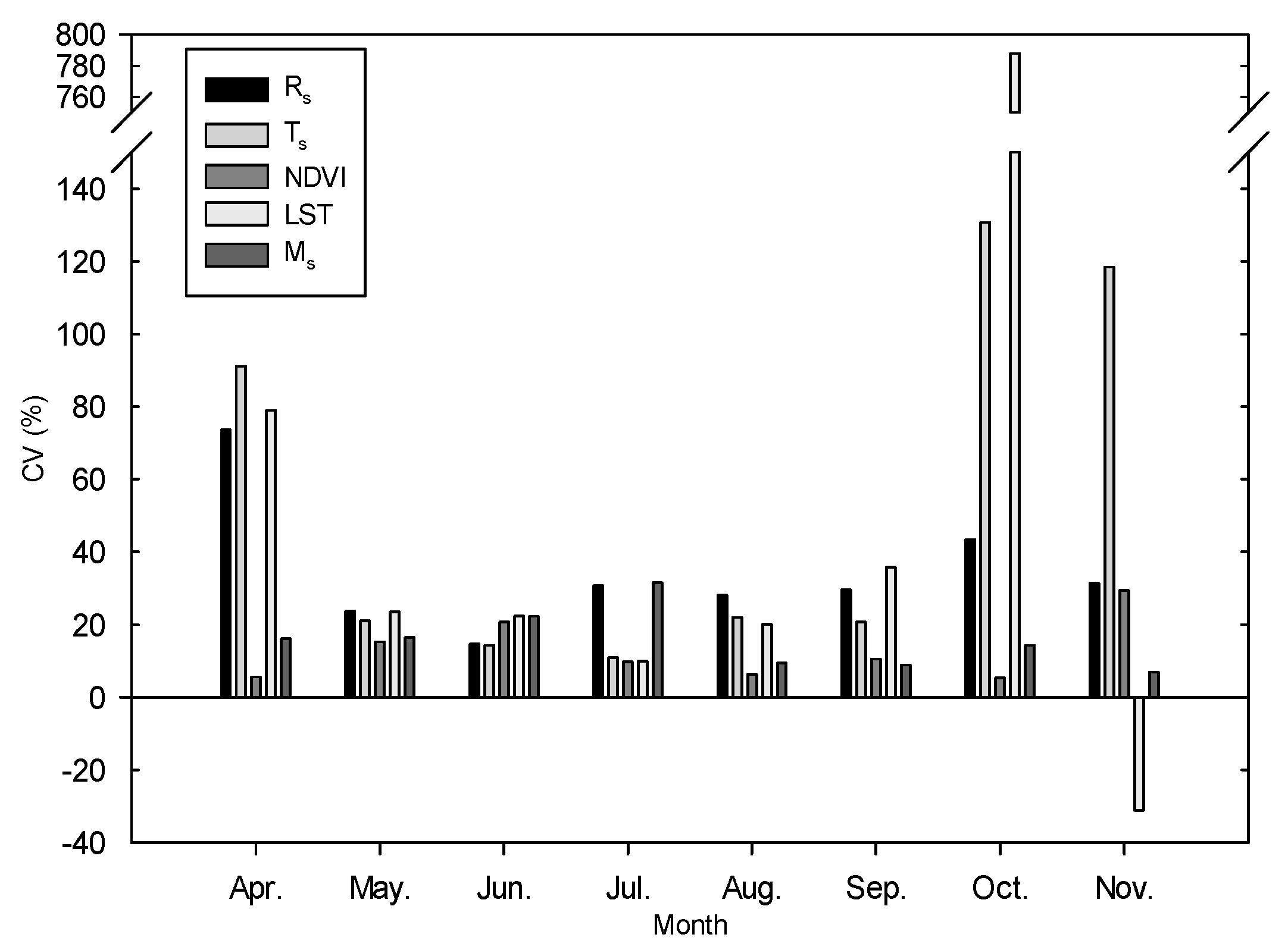
An overall preliminary correlation analysis showed that the soil temperature (Ts) at 5 cm and nighttime land surface temperature (LST) observed by MODIS onboard the Terra satellite correlated with soil respiration (Rs) best among all investigated temperature factors; therefore, we chose these two indexes as the representative temperature factors relating to Rs. As shown in Figure 2, during the measuring year, seasonal variations of Rs, Ts, NDVI, and LST were similar, with all of these generating an approximately symmetrical bell type distribution along the temporal scale. Owing to the effects of solar radiation, Ts was lowest in winter and spring (5.18 ± 2.36 °C in April) (mean ± SE), after which it dramatically increased as solar radiation and air temperature increased, reaching the highest value by the end of June and early July (17.38 ± 0.67 °C). Ts began to decrease in late July, with the greatest rate of decrease occurring from September to October. Additionally, the monthly coefficient of variation (CV) of Ts was comparatively higher in the phenological phase of the beginning and late growing period, while it maintained a low and steady value in the growing season (Figure 3). Under the influence of solar radiation and surface reflection, the seasonal variations in LST were in accordance with Ts, but comparatively lower. The maximum value of NDVI appeared from July to August, while its mean value during the measuring period was 0.55 ± 0.18 (mean ± SE), which was comparatively lower than other types of ecosystems (Figure 2c). In addition, the monthly CV of the NDVI was relatively low, being almost below 20% during each month. The seasonal dynamics of soil moisture (Ms) throughout the measuring period were not as pronounced as those for the other factors mentioned above. Rather, Ms showed a fluctuating pattern, accompanied by a trend of high and low alternations that varied significantly in response to natural precipitation. Overall, Ms was lower in late spring and early summer and higher in mid-summer, autumn and winter, with a mean value during the measuring period of 45.57% ± 8.09%. The monthly CVs of Ms and NDVI appeared to have a high and low fluctuating state within a small range, ranging from 6% in November to 31% in July for Ms and from 5% in October to 29% in November for NDVI (Figure 3).
Soil respiration exhibited an obvious bell type seasonal variation similar to Ts or LST, clearly illustrating the dynamics of Rs were closely related to temperature with time at the site. The Rs value was lower in the early growing season (1–2 μmol CO2 m−2 s−1), after which it gradually increased because of the rising temperature and biomass (4–8 μmol CO2 m−2 s−1), peaking at over 7 μmol CO2 m−2 s−1 in June and July. After that, Rs tapered gradually to less than 1 μmol CO2 m−2 s−1 in November. The mean value was 4.17 ± 0.29 μmol CO2 m−2 s−1 during the nine-year observation period. Additionally, the monthly CV of Rs exhibited a wave curve with time, ranging from 14% in June to 73% in April, with the maximum occurring in the spring and winter and the range being relatively smaller from May to November. The Rs rate presented a more stable state in June, when the CV was lowest (Figure 2a, Figure 3).

3.2. Modeling Rs Seasonal Variations

The relationship between Rs and environmental factors can be expressed by linear, exponential, double exponential, power, hyperbolic curve, quadratic, and Lloyd and Taylor models, as well as their composites. The linear and exponential models expressed the relationships between Rs and temperature or vegetation cover well. The model with the best fit was selected by comparing three model performance indicators (R2, RMSE, AIC). For the response of Rs to Ms, the quadratic equation had a better empirical fit. Correlation analyses showed that there was an extremely significantly positive correlation between Rs and Ts (r = 0.896**), LST (r = 0.834**) and NDVI (r = 0.753**) (Table 1), but no significant correlation between Rs and Ms. Overall, for the same environmental factors, the exponential model fitted better than the linear form, with higher R2 and lower RMSE and AIC values (Table 2). The exponential model based entirely on in situ measured Ts (R2 = 0.842, p < 0.001) showed a relatively higher explanation capacity than the exponential model based on LST (R2 = 0.762, p < 0.001). The further addition of Ms explained an additional 1.3% of the Rs seasonal variation based on the Ts linear model and 0.8% of the Rs seasonal variation based on the Ts exponential model. The model based entirely on the plant photosynthesis-related NDVI exhibited the poorest fit for Rs (R2 = 0.568 for the linear model, and R2 = 0.605 for the exponential model). However, the addition of LST improved the explanation by 15% for the linear model and 17.7% for the exponential model. Taking Ms, temperature and NDVI into account together, the explanation of the model showed a slight improvement relative to the exponential models with two variables. Overall, the model based on the in situ observed data had a slightly higher explanation than the model based on the spatial products, with higher R2 values and lower RMSE and AIC values. Considering that the three model performing indicators of three exponential models with good fitting effects (based on Ts, both Ts and Ms, and together with Ms, Ts, and NDVI) showed minor differences and the models all reached significant levels, we selected the simplest exponential model based on Ts as the optimum fitting model to describe seasonal variations in Rs.
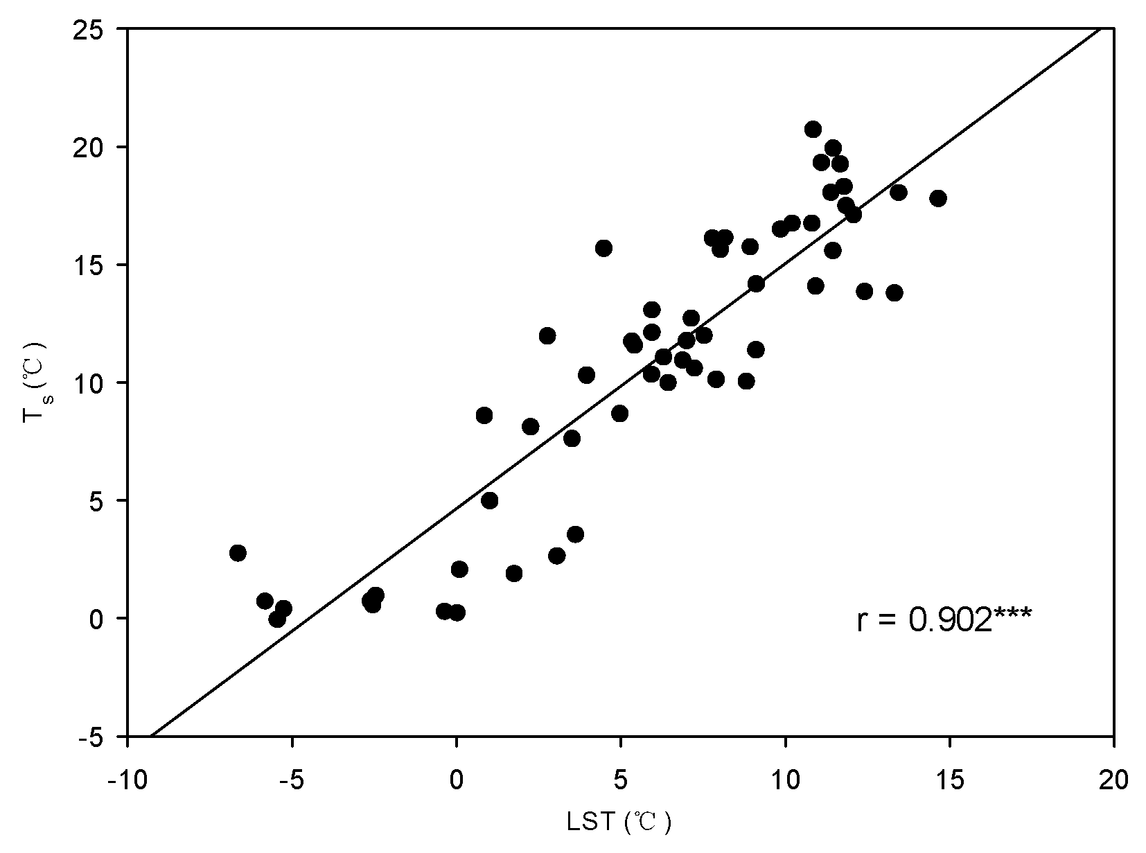
There was a small gap in the explanation capacity between the LST exponential model and the Ts exponential model, and the Pearson correlation coefficient was 0.902 between Ts and LST data (Figure 4). A univariate exponential model based on Ts and LST was then constructed for each year (Table 3). The t-test analysis of the three model performance indicators of two univariate exponential models for each year produced no significant differences. Therefore, the LST exponential model based on complete remote sensing data could be used as an empirical fitting model to modify seasonal variations in Rs.
The modeling accuracy of the Rs predictive models based on the Ts exponential equation and LST exponential equation is presented in Figure 5 (a for Ts; b for LST). Pearson’s correlation coefficient was 0.862** between the measured Rs and predicted Rs based on Ts and 0.807** between the measured Rs and predicted Rs based on the LST, verifying that the Ts and LST data were both effective and reliable for prediction of the temporal variations in Rs in the study site.

3.3. Temperature Sensitivity of Rs

The seasonal trend of Q10 and other climatic factors differed. Specifically, the monthly Ts and Rs increased from April (5.18 ± 2.34 °C, 2.53 ± 0.93 μmol CO2 m−2 s−1) to July (17.38 ± 0.67 °C, 6.29 ± 0.68 μmol CO2 m−2 s−1), after which they decreased to the lowest values in November (0.91 ± 0.48 °C, 0.84 ± 0.12 μmol CO2 m−2 s−1) (Figure 6). The Q10 seasonal trend was contrary to the corresponding Ts and Rs trends, presenting a concave type distribution. Moreover, its value was higher in cold months and lower in warm months. The Q10 value decreased from April (4.31) to September (1.27), then increased dramatically until peaking in November (7.03). The seasonal R10 trend fluctuated, but its values basically remained around 4 μmol CO2 m−2 s−1 during each month.
Under different temperature conditions, Q10 presented obviously different values (Figure 7). Specifically, as temperatures decreased, Q10 became higher. At the temperature interval of −1 °C to 5 °C, the Q10 value was 7.61, with a mean Ts of 1.5 °C and a mean Rs of 1.25 μmol CO2 m−2 s−1. The Q10 then decreased dramatically with the same temperature interval, i.e., Q10 value of 0.67 for a temperature interval of 5 °C–11 °C (mean Ts of 9.53 °C, Rs of 3.21 μmol CO2 m−2 s−1), 1.79 for a temperature interval of 11 °C–16 °C (mean Ts of 13.18 °C, Rs of 4.86 μmol CO2 m−2 s−1), and 1.28 for 16 °C–21 °C (mean Ts of 17.84 °C, Rs of 6.29 μmol CO2 m−2 s−1). Overall, Rs was extremely sensitive to temperature changes at lower temperatures.
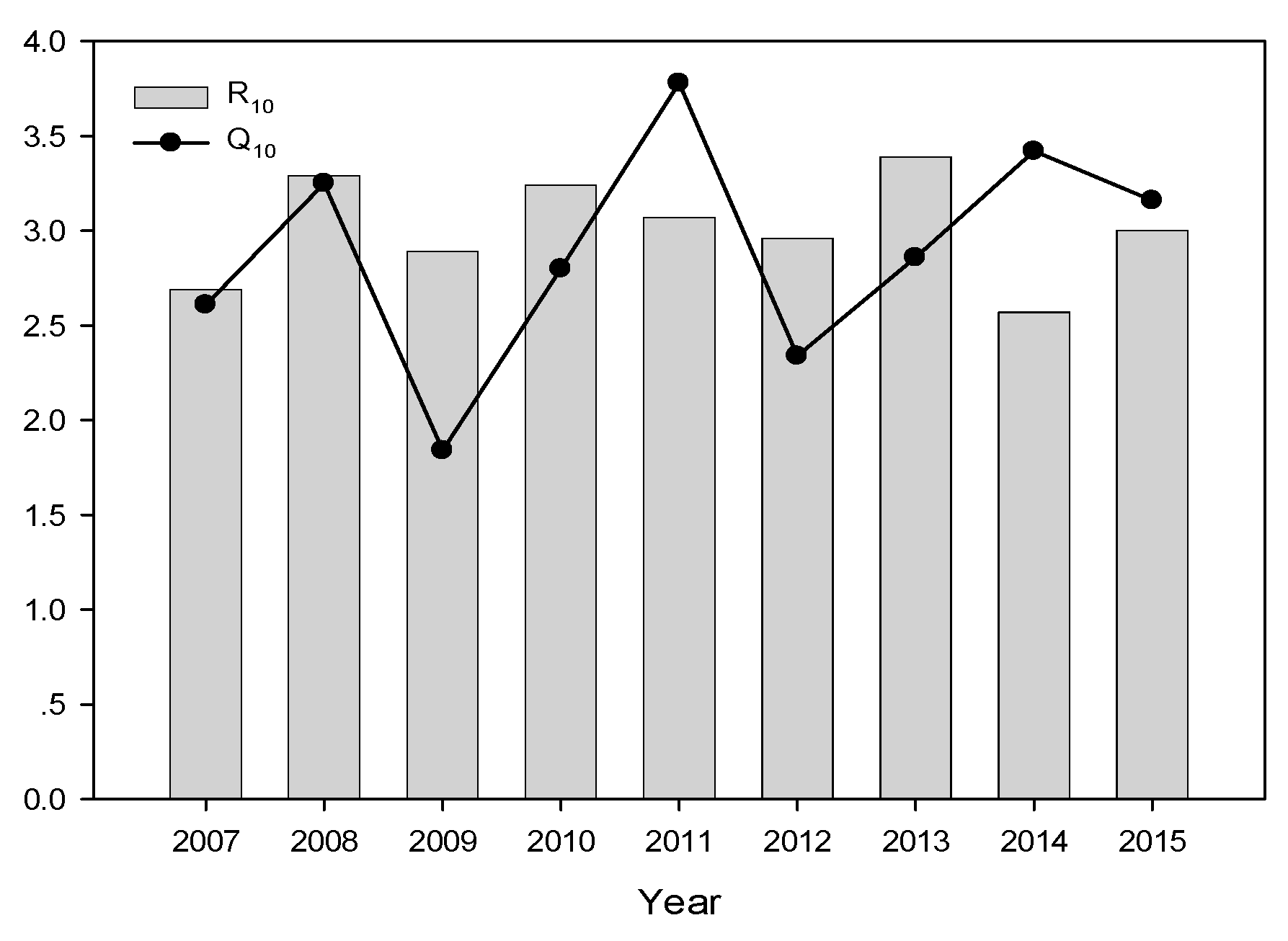
The R10 values in each year presented a fluctuating trend, ranging from a minimum of 2.57 μmol CO2 m−2 s−1 in 2014 to a maximum of 3.39 μmol CO2 m−2 s−1 in 2013. The CV value was 9% during the nine-year observation period (Figure 8). Additionally, the mean annual R10 was 3.01 ± 0.27 μmol CO2 m−2 s−1. The annual Q10 values showed a trend of fluctuation as well, but its range was greater than that of R10, with a minimum of 1.84 being observed in 2009 and a maximum of 3.78 in 2011. The yearly CV was 20% and the mean value of Q10 during the study year was 2.90 ± 0.59. Overall, although the R10 and Q10 values differed during each observed year, they were close to the mean values, except in 2009, when there was a water stress during the summer. This water shortage led to especially strong variations in Q10.

4. Discussion

4.1. Seasonal Variations in Rs

The seasonal patterns of Rs, Ts, LST, and NDVI all showed symmetrical bell type distributions, while Ms fluctuated during the nine-year measuring time. The variation in Rs was consistent with that of the temperature (Ts, LST), illustrating that temperature could explain most of the temporal variation of Rs. Mo et al. [30] observed a similar trend in the daily mean soil temperature at 1 cm depth and daily CO2–C efflux, and a fluctuating trend of Ms at 15 cm depth among the four surveyed years of 1999–2002 in a cool-temperate deciduous broad-leaved forest in Japan. Zhang et al. [31] found that the seasonal variation of Rs was not completely consistent with the daily mean Ts of the upper 10 cm and that variations in Rs followed GPP during most of the growing seasons in a wheat and maize rotation cropland in the North China Plain. The present study site was a sub-alpine meadow; accordingly, the amount of biomass was very small. Moreover, obvious vegetation degradation due to anthropogenic activities has occurred in the region in recent years. Therefore, biomass had a relatively smaller effect on Rs in the study site, with the temporal variation of Rs being not completely consistent with that of NDVI. The correlation analysis of all measured data (analysis not shown) revealed that the correlation between Rs and Ts became lower as soil depth increased (T5 > T10 > T15), indicating that the soil respiration rate was more influenced by the soil temperature close to the surface. Since there was no forest cover in the study site, the soil temperature was completely controlled by changes in solar radiation. A lagging phenomenon in which the soil temperature at greater depth showed obvious time hysteresis when compared with the soil temperature near the surface was observed by Huang et al. [23]. The LSTtn (nighttime LST from the Terra satellite) captured the seasonal variation of Rs best among all the MODIS eight-day LST products in the study site during the nine-year period, which was consistent with the results of other studies. Huang et al. [22] selected the nighttime LST observed by the Terra satellite to estimate Rs at 2 contrasting forest sites, while Huang et al. [23] chose the average LST of daytime and nighttime data from MOD11A2 as a driver of the Rs fitting model of a deciduous broadleaf forest in the midwestern United States. Wu et al. [5] reported that the nighttime LST from the Terra satellite was better correlated with the soil respiration than the daytime LST at a Canadian boreal black spruce stand and indicated that the nighttime LST could be a better estimate of the baseline temperature that regulated plant phenology. These results confirmed that the nighttime land surface temperature data from the MODIS eight-day spatial products captured Rs variation reliably. Mo et al. [30] demonstrated that the Rs of 0 °C soil temperature at –1 cm was higher during autumn than spring because the active soil layer remained large as the deeper soil layers warmed up in the summer. Widen [32] also found that the Rs of 0 °C soil temperature was higher during the highest fine-root production period from July to September. Because of the higher altitude of the study site, measurements could not be operated because of the snow cover and cold temperature from December to March. The spring in north China is short, and the air temperature rises rapidly in May. As a result, the Rs in April was lower, while it obviously increased in May and June. In October, the temperature dropped sharply, resulting in the Rs being significantly lower than in September. The soil moisture affected root growth, soil microbial activity, and soil metabolic activity, and therefore influenced Rs. Seasonal variations of Ms at the study site were mainly affected by precipitation. Unlike the obvious seasonal variations in Ts, Ms seasonal variations throughout the measuring period fluctuated between high and low levels. After the precipitation, Ms increased rapidly, but then decreased until the next occurrence of precipitation because of water infiltration, soil evaporation, and plant transpiration. When compared to the relationship between Rs and temperature, that of Rs and Ms was relatively complex and uncertain because the response of Rs to Ms differed during different stages [6]. Under dry soil conditions, the soil biochemistry metabolic activity became frequent as the soil water content improved. When Ms reached 50%–80% of the soil saturated water content, the maximum soil microbial metabolic activity was reached and the Rs rate achieved the largest value. As Ms continued to increase, the lack of oxygen prevented aerobic respiration. Therefore, in a certain range of Ms, the relationship between the Rs rate and Ms was positively correlated, and when Ms goes over a certain range, with the increase of Ms, Rs decreased. Precipitation and drought could affect the relationship between Rs and Ms, with rainfall increasing Rs under drought conditions and reducing it under humid conditions. The Ms in the study site was in the range of 35%–55%; therefore, there was virtually no stress of Ms on Rs. The changes in Ms in such a narrow range did not have a significant effect on Rs rate during the measuring years. However, in July of 2009, Rs was significantly lower than in the same period of other years. Specifically, the value of Ts, Ms, and Rs during this period was 17.45 °C, 15.78%, and 4.45 μmol CO2 m−2 s−1, respectively, while in the same period of other measuring years, Ts was around 18 °C, Ms was around 45%, and Rs was about 7 μmol CO2 m−2 s−1. It can be seen that Ts value was close to each other, while the difference between Ms in July of 2009 and during other years was about 30%, indicating that Rs was inhibited by water stress in July of 2009.

4.2. Factors Affecting the Seasonal Variations of Rs

The spatial scales of MODIS data were widely apart, i.e., 500 m for vegetation indices and 1000 m for LST, respectively. As the average spatially-distributed observed Rs data represented the mean value of the study site determined by analysis of spatial heterogeneity [25,26], the MODIS products (i.e., LST and NDVI) can be considered to be consistent with the in situ measured data (i.e., Rs, Ts, and Ms) in spatial matching. Moreover, some previous studies have verified the spatial matching of MODIS spatial products and the observation of eddy flux towers [23]. The seasonal variations in Rs may be related to temporal changes in temperature, soil moisture, and other soil physicochemical factors (i.e., SOC, N, pH, etc.), as well as changes in the phenology of biotic factors (i.e., plant photosynthesis and its development phase, fine root production, microbial activity, and below-ground C allocation) [14,19,30,31,33]. Soil physical and chemical factors were basically constant on temporal scale in the study site. We selected the most influential environmental factors to model seasonal variations in Rs. The capacity of the exponential model to explain the same independent environmental variables was significantly higher than that of the linear model. Based on the R2, RMSE, and AIC, a statistically significant difference was not detected among well fitted exponential-type functions considering Ts alone, Ts and Ms, or Ts, Ms and NDVI together. The soil water supply was generally sufficient in the study site; therefore, adding it into the fitting model did not significantly improve the model explanatory capacity. Moreover, the addition of NDVI did not greatly improve the explanation capacity, possibly because of the lower above-ground biomass in the study site. The exponential function driven by Ts was selected as the best fitted model to estimate the seasonal variations of Rs in the study site as it needed only one unknown independent variable. This finding indicated that the contribution of the soil moisture and vegetation index to Rs was relatively small and temperature exerted the greatest control on Rs in the study site. In another alpine meadow on the Tibetan Plateau, Hu et al. [34] found that soil temperature and above-ground biomass rather than soil moisture mainly affected the ecosystem respiration. Findings of the present study were in agreement with those of previous studies that showed Rs was most sensitive to the soil temperature among all related environmental factors on a temporal scale [8,13,35], on account of the principle that soil temperature acted as a dominant climatic factor on Rs alongside impact substrate and physiological activities, which ultimately affected Rs. Therefore, temperature could be a reliable predictor for the seasonal variation in Rs. However, several studies have shown that Rs was most closely related to the soil moisture under dry conditions [36]. It depends on which factor is the limiting factor in any given ecosystem. In the present study, Ms was sufficient, so its impact on Rs was smaller. Therefore, the decisive driver of Rs was not the same under different environmental conditions. The unexplained Rs seasonal variation based on our selected model may have been due to the microbial properties and soil physical and chemical properties related to Rs, since the addition of Ms and NDVI did not significantly improve the explanatory power. The model driven only by temperature may have masked several biotic processes (e.g., plant photosynthesis and microbial activities), abiotic processes (e.g., water supply) and their combined effects [22,37], but it also avoided the multi-collinearity problems among the independent variables and the increasing uncertainty of model based predictions caused by increases in independent variables [22]. For example, soil temperature influenced root respiration and microbial activities [38], soil moisture influenced the physiological processes of roots and microorganisms [39], etc. The R2 value of the exponential model driven by LST was 0.762***, which was slightly lower than the R2 value of the Ts exponential model (0.842***), indicating that LST also provided useful information for fitting seasonal variations in Rs. The t-test analysis of modeling performing indicators (i.e., R2, RMSE, and AIC) in each year of the two best fitted one-variable exponential model showed that there was no significant difference between the Ts exponential model and the LST exponential model. These findings confirmed the potential role of remote sensing data to estimate the seasonal variations in Rs on a regional scale [5,14,22,23,37]. Moreover, these results validated the applicability of spatial data products in Rs temporal dynamic modeling and provided data support for estimating Rs using spatial data products on a large scale.

4.3. Temperature Sensitivity of Rs

Previous studies have mostly focused on the relationship between Rs and its related environmental factors, and Q10 has been studied as an index to evaluate the temperature sensitivity of Rs. Moreover, some researchers have studied the environmental factors affecting Q10 [2]. In the study site, the seasonal variations in the soil respiration sensitivity index, Q10, showed a curve opposite to that of Rs and Ts with hysteresis. Despite considering the fact that Q10 was controlled by the soil temperature, soil moisture [40], organic matter decomposition [41], soil physical and chemical properties and biotic factors such as vegetation cover and fine root mass [19], also varied depending on the location [13], the differences among monthly Q10 values may mainly be controlled by the combination of soil moisture and soil temperature because of the relatively constant soil physical and chemical properties in study site.
The Q10 values for different temperature intervals indicated a negative response of Q10 to Rs and Ts in accordance with previously published studies [1,2,40,42]. The physical and bio-chemical process consisting of Rs was constrained by lower temperatures; thus, an increase of temperature could significantly improve the soil respiration rate, resulting in a higher Q10 at lower temperatures. However, under higher temperatures that had met the need of Rs, further increases in temperature did not improve Rs, resulting in a lower Q10 [43]. The Q10 acclimated to the soil temperature because of the sufficient soil moisture in the study site. The annual Q10 values ranged from 1.84 to 3.78 with a mean value of 2.90 ± 0.59, which were slightly higher than the global mean of 2.4 and range of 1.3 to 3.3 [44]. The temperature in the study site was much lower because of the high altitude, and the actual Q10 value may have been slightly higher than the calculated mean value because of the missing data for the coldest days when the measurements could not be taken. Within the soil temperature range of −0.1 °C to 20.68 °C of the nine-year measured data, the Q10 value based on all measured data was approximately 3.08, which was almost equal to the mean Q10 value (2.90 ± 0.59) of the annual Q10. It should be noted that the Q10 value was quite low under water stress in 2009, indicating that the response of Rs to temperature was obviously inhibited by water stress when there was a low water supply. The R10 value (3.01 ± 0.27 μmol CO2 m−2 s−1) in the study site was comparable to that of other studies, such as 1.27–2.90 for 11 sites with four types of land cover in a mountain area investigated by Li et al. [19] and 2.30–3.60 in a temperate deciduous forest studied by Vincent et al. [45].

5. Conclusions

The findings present that soil temperature near the surface soil exerts dominant control on soil respiration rate at a seasonal scale due to the lower above-ground biomass and sufficient soil moisture supply. The seasonal variations in Rs can be effectively estimated based on the proposed Ts-exponential model in the study area. Also, the high explanation capacity of the LST-exponential model highlights a promising prospect of applying the remote sensing products to the seasonal estimating model of Rs during further exploration. The Q10 seasonal variation presents a concave type distribution, with its value significantly controlled by temperature under lower temperature conditions. The results presented herein demonstrate the determining role of temperature in Rs seasonal variations in a sub-alpine meadow zone and quantitively verify the applicability of spatial data products for estimating Rs temporal variations.

Author Contributions

Conceptualization, Y.L., Y.C. and J.Y.; data curation, Y.L., J.Y. and H.L.; formal analysis, Y.L.; investigation, Y.L. and H.L.; supervision, H.L.; writing—original draft, Y.L.; writing—review and editing, Y.C.; funding acquisition, Y.C. and J.Y.

Funding

This research was funded by the National Key Research Program of China (Grant No. 2016YFC0502209), the National Natural Science Foundation of China (Grant No. 51522901, Grant No. 41201374) and the Fundamental Research Funds for the Central Universities.

Acknowledgments

We would like to express our gratitude to the anonymous reviewers and the editors for providing us the valuable comments and suggestions in improving our manuscript.

Conflicts of Interest

The authors declare no conflict of interest.

References

  1. Han, M.G.; Jin, G.Z. Seasonal variations of Q(10) soil respiration and its components in the temperate forest ecosystems, northeastern China. Eur. J. Soil Biol. 2018, 85, 36–42. [Google Scholar] [CrossRef]
  2. Zhao, K.J.; Dong, B.Q.; Jia, Z.K.; Ma, L. Effect of climatic factors on the temporal variation of stem respiration in Larix principis-rupprechtii Mayr. Agric. For. Meteorol. 2018, 248, 441–448. [Google Scholar] [CrossRef]
  3. Zhao, Y.L.; Goldberg, S.D.; Xu, J.C.; Harrison, R.D. Spatial and seasonal variation in soil respiration along a slope in a rubber plantation and a natural forest in Xishuangbanna, Southwest China. J Mt. Sci. 2018, 15, 695–707. [Google Scholar] [CrossRef]
  4. Ohashi, M.; Gyokusen, K. Temporal change in spatial variability of soil respiration on a slope of Japanese cedar (Cryptomeria japonica D. Don) forest. Soil Biol. Biochem. 2007, 39, 1130–1138. [Google Scholar] [CrossRef]
  5. Wu, C.Y.; Gaumont-Guay, D.; Black, T.A.; Jassal, R.S.; Xu, S.G.; Chen, J.M.; Gonsamo, A. Soil respiration mapped by exclusively use of MODIS data for forest landscapes of Saskatchewan, Canada. ISPRS J. Photogramm. Remote Sens. 2014, 94, 80–90. [Google Scholar] [CrossRef]
  6. Raich, J.W.; Potter, C.S. Global Patterns of Carbon-Dioxide Emissions from Soils. Glob. Biogeochem. Cycle 1995, 9, 23–36. [Google Scholar] [CrossRef]
  7. Foti, S.; Balogh, J.; Nagy, Z.; Herbst, M.; Pinter, K.; Peli, E.; Koncz, P.; Bartha, S. Soil moisture induced changes on fine-scale spatial pattern of soil respiration in a semi-arid sandy grassland. Geoderma 2014, 213, 245–254. [Google Scholar] [CrossRef]
  8. Munoz-Rojas, M.; Lewandrowski, W.; Erickson, T.E.; Dixon, K.W.; Merritt, D.J. Soil respiration dynamics in fire affected semi-arid ecosystems: Effects of vegetation type and environmental factors. Sci. Total Environ. 2016, 572, 1385–1394. [Google Scholar] [CrossRef]
  9. Bond-Lamberty, B.; Thomson, A. Temperature-associated increases in the global soil respiration record. Nature 2010, 464, 579. [Google Scholar] [CrossRef]
  10. Zeng, X.H.; Song, Y.G.; Zhang, W.J.; He, S.B. Spatio-temporal Variation of Soil Respiration and Its Driving Factors in Semi-arid Regions of North China. Chin. Geogr. Sci. 2018, 28, 12–24. [Google Scholar] [CrossRef]
  11. Ahmad, W.; Singh, B.; Dijkstra, F.A.; Dalal, R.C.; Geelan-Small, P. Temperature sensitivity and carbon release in an acidic soil amended with lime and mulch. Geoderma 2014, 214, 168–176. [Google Scholar] [CrossRef]
  12. Ahmad, W.; Singh, B.; Dijkstra, F.A.; Dalal, R.C. Inorganic and organic carbon dynamics in a limed acid soil are mediated by plants. Soil Biol. Biochem. 2013, 57, 549–555. [Google Scholar] [CrossRef]
  13. Lloyd, J.; Taylor, J.A. On the temperature-dependence of soil respiration. Funct. Ecol. 1994, 8, 315–323. [Google Scholar] [CrossRef]
  14. Sanchez, M.L.; Ozores, M.I.; Lopez, M.J.; Colle, R.; De Torre, B.; Garcia, M.A.; Perez, I. Soil CO2 fluxes beneath barley on the central Spanish plateau. Agric. For. Meteorol. 2003, 118, 85–95. [Google Scholar] [CrossRef]
  15. Borken, W.; Xu, Y.J.; Brumme, R.; Lamersdorf, N. A climate change scenario for carbon dioxide and dissolved organic carbon fluxes from a temperate forest soil: Drought and rewetting effects. Soil Sci. Soc. Am. J. 1999, 63, 1848–1855. [Google Scholar] [CrossRef]
  16. Birch, H.F. The effect of soil drying on humus decomposition and nitrogen availability. Plant Soil 1958, 10, 9–31. [Google Scholar] [CrossRef]
  17. Ahmad, W.; Singh, B.; Dalal, R.C.; Dijkstra, F.A. Carbon dynamics from carbonate dissolution in Australian agricultural soils. Soil Res. 2015, 53, 144–153. [Google Scholar] [CrossRef]
  18. Samuelson, L.; Mathew, R.; Stokes, T.; Feng, Y.C.; Aubrey, D.; Coleman, M. Soil and microbial respiration in a loblolly pine plantation in response to seven years of irrigation and fertilization. For. Ecol. Manag. 2009, 258, 2431–2438. [Google Scholar] [CrossRef]
  19. Li, H.J.; Yan, J.X.; Yue, X.F.; Wang, M.B. Significance of soil temperature and moisture for soil respiration in a Chinese mountain area. Agric. For. Meteorol. 2008, 148, 490–503. [Google Scholar] [CrossRef]
  20. Zhang, Q.; Katul, G.G.; Oren, R.; Daly, E.; Manzoni, S.; Yang, D.W. The hysteresis response of soil CO2 concentration and soil respiration to soil temperature. J. Geophys. Res. Biogeosci. 2015, 120, 1605–1618. [Google Scholar] [CrossRef]
  21. Huang, N.; Niu, Z. Estimating soil respiration using spectral vegetation indices and abiotic factors in irrigated and rainfed agroecosystems. Plant Soil 2013, 367, 535–550. [Google Scholar] [CrossRef]
  22. Huang, N.; Gu, L.H.; Black, T.A.; Wang, L.; Niu, Z. Remote sensing-based estimation of annual soil respiration at two contrasting forest sites. J. Geophys. Res. Biogeosci. 2015, 120, 2306–2325. [Google Scholar] [CrossRef] [Green Version]
  23. Huang, N.; Gu, L.H.; Niu, Z. Estimating soil respiration using spatial data products: A case study in a deciduous broadleaf forest in the Midwest USA. J. Geophys. Res. Atmos. 2014, 119, 6393–6408. [Google Scholar] [CrossRef]
  24. Suqing, L.I.; Jintun, Z. Ecological analysis of subalpine meadow in Yunding Mountain, Shanxi. Geogr. Res. 2007, 26, 83–90. [Google Scholar]
  25. Yan, J.-X.; Li, J.-J.; Li, H.-J.; Zhang, Y.-H. Studies on spatial heterogeneity of soil respiration in a subalpine meadow. Huanjing Kexue 2013, 34, 3992–3999. [Google Scholar] [PubMed]
  26. Li, H.-J.; Gao, Y.-F.; Yan, J.-X.; Li, J.-J. Spatial heterogeneity of soil respiration in a subalpine meadow at different sampling scales. Huanjing Kexue 2014, 35, 4313–4320. [Google Scholar] [PubMed]
  27. Wan, Z.M. New refinements and validation of the MODIS Land-Surface Temperature/Emissivity products. Remote Sens. Environ. 2008, 112, 59–74. [Google Scholar] [CrossRef]
  28. Huang, N.; He, J.S.; Niu, Z. Estimating the spatial pattern of soil respiration in Tibetan alpine grasslands using Landsat TM images and MODIS data. Ecol. Indic. 2013, 26, 117–125. [Google Scholar] [CrossRef]
  29. Rouse, J.W.; Haas, R.H.; Schell, J.A.; Deering, D.W.; Harlan, J.C. Monitoring the Vernal Advancements and Retrogradation of Natural Vegetation; Texas A & M University, Remote Sensing Center: Greenbelt, MD, USA, 1974. [Google Scholar]
  30. Mo, W.; Lee, M.S.; Uchida, M.; Inatomi, M.; Saigusa, N.; Mariko, S.; Koizumi, H. Seasonal and annual variations in soil respiration in a cool-temperate deciduous broad-leaved forest in Japan. Agric. For. Meteorol. 2005, 134, 81–94. [Google Scholar] [CrossRef]
  31. Zhang, Q.; Lei, H.M.; Yang, D.W. Seasonal variations in soil respiration, heterotrophic respiration and autotrophic respiration of a wheat and maize rotation cropland in the North China Plain. Agric. For. Meteorol. 2013, 180, 34–43. [Google Scholar] [CrossRef]
  32. Widen, B. Seasonal variation in forest-floor CO2 exchange in a Swedish coniferous forest. Agric. For. Meteorol. 2002, 111, 283–297. [Google Scholar] [CrossRef]
  33. Kato, T.; Tang, Y.H.; Gu, S.; Cui, X.Y.; Hirota, M.; Du, M.Y.; Li, Y.N.; Zhao, Z.Q.; Oikawa, T. Carbon dioxide exchange between the atmosphere and an alpine meadow ecosystem on the Qinghai-Tibetan Plateau, China. Agric. For. Meteorol. 2004, 124, 121–134. [Google Scholar] [CrossRef]
  34. Hu, Y.G.; Jiang, L.L.; Wang, S.P.; Zhang, Z.H.; Luo, C.Y.; Bao, X.Y.; Niu, H.S.; Xu, G.P.; Duan, J.C.; Zhu, X.X.; et al. The temperature sensitivity of ecosystem respiration to climate change in an alpine meadow on the Tibet plateau: A reciprocal translocation experiment. Agric. For. Meteorol. 2016, 216, 93–104. [Google Scholar] [CrossRef]
  35. Jenkins, M.E.; Adams, M.A. Respiratory quotients and Q(10) of soil respiration in sub-alpine Australia reflect influences of vegetation types. Soil Biol. Biochem. 2011, 43, 1266–1274. [Google Scholar] [CrossRef]
  36. Moyano, F.E.; Manzoni, S.; Chenu, C. Responses of soil heterotrophic respiration to moisture availability: An exploration of processes and models. Soil Biol. Biochem. 2013, 59, 72–85. [Google Scholar] [CrossRef]
  37. Huang, N.; Niu, Z.; Zhan, Y.L.; Xu, S.G.; Tappert, M.C.; Wu, C.Y.; Huang, W.J.; Gao, S.; Hou, X.H.; Cai, D.W. Relationships between soil respiration and photosynthesis-related spectral vegetation indices in two cropland ecosystems. Agric. For. Meteorol. 2012, 160, 80–89. [Google Scholar] [CrossRef]
  38. Wan, S.; Norby, R.J.; Ledford, J.; Weltzin, J.F. Responses of soil respiration to elevated CO2, air warming, and changing soil water availability in a model old-field grassland. Glob. Chang. Biol. 2007, 13, 2411–2424. [Google Scholar] [CrossRef]
  39. Huang, G.; Li, Y.; Su, Y.G. Effects of increasing precipitation on soil microbial community composition and soil respiration in a temperate desert, Northwestern China. Soil Biol. Biochem. 2015, 83, 52–56. [Google Scholar] [CrossRef]
  40. Jiang, J.S.; Guo, S.L.; Zhang, Y.J.; Liu, Q.F.; Wang, R.; Wang, Z.Q.; Li, N.N.; Li, R.J. Changes in temperature sensitivity of soil respiration in the phases of a three-year crop rotation system. Soil Tillage Res. 2015, 150, 139–146. [Google Scholar] [CrossRef]
  41. Davidson, E.A.; Janssens, I.A. Temperature sensitivity of soil carbon decomposition and feedbacks to climate change. Nature 2006, 440, 165–173. [Google Scholar] [CrossRef]
  42. Janssens, I.A.; Pilegaard, K. Large seasonal changes in Q(10) of soil respiration in a beech forest. Glob. Chang. Biol. 2003, 9, 911–918. [Google Scholar] [CrossRef]
  43. Andrews, J.A.; Matamala, R.; Westover, K.M.; Schlesinger, W.H. Temperature effects on the diversity of soil heterotrophs and the delta C-13 of soil-respired CO2. Soil Biol. Biochem. 2000, 32, 699–706. [Google Scholar] [CrossRef]
  44. Raich, J.W.; Schlesinger, W.H. The global carbon-dioxide flux in soil respiration and its relationship to vegetation and climate. Tellus Ser. B Chem. Phys. Meteorol. 1992, 44, 81–99. [Google Scholar] [CrossRef]
  45. Vincent, G.; Shahriari, A.R.; Lucot, E.; Badot, P.M.; Epron, D. Spatial and seasonal variations in soil respiration in a temperate deciduous forest with fluctuating water table. Soil Biol. Biochem. 2006, 38, 2527–2535. [Google Scholar] [CrossRef]
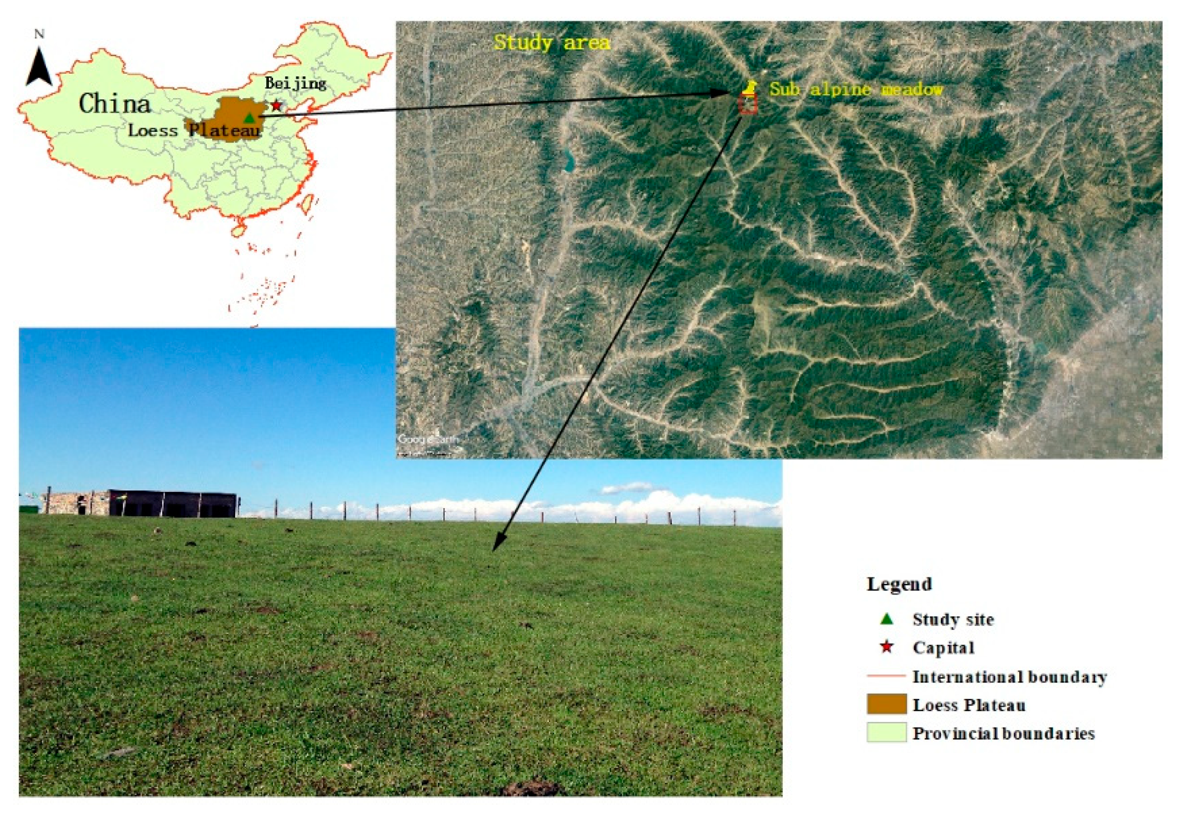
Figure 1. A sketch map of the study area in the Loess Plateau, China.
Sustainability 11 03274 g001
Figure 2. Seasonal dynamics of (a) soil respiration (Rs), (b) soil temperature (Ts), nighttime land surface temperature (LST) observed by Terra satellite, (c) normalized difference vegetation index (NDVI), and (d) soil moisture (Ms) in the sub-alpine meadow from 2007 to 2015.
Sustainability 11 03274 g002
Figure 3. The monthly coefficient of variation (CV) of soil respiration (Rs), soil temperature (Ts), nighttime land surface temperature (LST) observed by Terra satellite, normalized difference vegetation index (NDVI), and soil moisture (Ms) from 2007 to 2015.
Sustainability 11 03274 g003
Figure 4. Relationships between soil temperature (Ts) and land surface temperature (LST) in study site from 2007 to 2015 (n = 58). *** means the relationships are statistically significant at p < 0.001.
Sustainability 11 03274 g004
Figure 5. The relationship between measured soil respiration (measured Rs) and (a) Ts exponential model estimated soil respiration (estimated Rs), and (b) LST exponential model estimated soil respiration (estimated Rs). ** correlation is significant at 0.01 level (two-tailed).
Sustainability 11 03274 g005
Figure 6. Seasonal variation of the monthly mean temperature sensitivity (Q10) with (a) soil respiration (Rs), reference soil respiration (R10), and (b) soil temperature (Ts) from 2007 to 2015 in study site. Error bars indicate the standard error.
Sustainability 11 03274 g006
Figure 7. Temperature sensitivity of soil respiration (Q10) with (a) soil respiration (Rs) and (b) soil temperature (Ts) in different temperature intervals. Error bars indicate the standard errors.
Sustainability 11 03274 g007
Figure 8. Reference soil respiration (R10) and temperature sensitivity of soil respiration (Q10) derived from the exponential equations in each year.
Sustainability 11 03274 g008
Table 1. Correlation coefficients (r) and p values between soil respiration (Rs) and its related factors.
Rs RsTsMsLSTNDVI
r1.0000.896 **−0.1830.834 **0.753 **
p value 0.0000.1690.0000.000
** Correlation is significant at 0.01 level (two-tailed); n = 58. Rs is measured soil respiration (μmol CO2 m−2s−1), Ts is soil temperature (°C), LST is the nighttime land surface temperature observed by the Moderate Resolution Imaging Spectro radiometer (MODIS) onboard terra satellite (°C), and NDVI is the normalized difference vegetation index.
Table 2. Regression analysis relating soil respiration (Rs) to soil temperature (Ts), soil moisture (Ms), land surface temperature (LST), and the normalized difference vegetation index (NDVI).
Models and EquationsR2RSSRMSEAIC
R s = f ( T s ) (1) R s = a T s + b 0.803 ***56.2860.9852.260
(2) R s = a e b T s 0.842 ***4.7420.286−141.231
R s = f ( M s · T s ) (1) R s = a M s + b M s 2 + c T s + d 0.816 ***52.610.9520.343
(2) R s = a exp ( b M s + c M s 2 + d T s ) 0.850 ***4.4990.279−142.282
R s = f ( LST ) (1) R s = a LST + b 0.695 ***87.1351.22627.607
(2) R s = a e b LST 0.762 ***7.1350.351−117.535
R s = f ( NDVI ) (1) R s = a NDVI + b 0.568 ***123.7011.46047.931
(2) R s = a e b NDVI 0.605 ***11.8230.451−88.243
R s = f ( LST · NDVI ) (1) R s = a LST + b NDVI + c 0.718 ***80.5621.17925.058
(2) R s = a exp ( b LST + c NDVI ) 0.782 ***6.5370.336−120.612
R s = f ( M s · T s · NDVI ) (1) R s = a M s + b M s 2 + c T s + d NDVI + e 0.817 ***52.4190.9512.132
(2) R s = a exp ( b M s + c M s 2 + d T s + e NDVI ) 0.854 ***4.3640.274−142.049
R s = f ( M s · LST · NDVI ) (1) R s = a M s + b M s 2 + c LST + d NDVI + e 0.748 ***72.0851.11520.609
(2) R s = a exp ( b M s + c M s 2 + d LST + e NDVI ) 0.819 ***5.4310.306−129.363
R2 is the coefficient of determination, RMSE (μmol CO2 m−2s−1) is the root-mean-square error, and AIC is the Akaik’s information criterion. *** means the relationships are statistically significant at p < 0.001. Rs is measured soil respiration (μmol CO2 m−2s−1), Ts is soil temperature (°C), LST is the nighttime land surface temperature observed by the Moderate Resolution Imaging Spectro radiometer (MODIS) onboard terra satellite (°C), and NDVI is the normalized difference vegetation index.
Table 3. The model evaluation index of two univariate exponential models in each year in the study site.
200820092010201120122013201420152007–2015
R210.9070.6010.8850.9410.6760.7970.9130.9230.842
R220.9470.5540.6880.9840.7040.6570.8920.7570.762
RMSE10.2110.3300.2160.2210.3260.2820.2520.1790.286
RMSE20.1590.3500.3840.1220.3360.3960.3040.3660.351
AIC1−14.674−9.289−17.425−17.152−11.710−13.705−15.289−23.567−141.231
AIC2−18.054−8.614−10.461−26.477−12.352−10.040−13.730−14.391−117.535
R2 was the determination coefficient of the model and it reached 0.05 significance level in each year. RMSE (μmol CO2 m−2s−1) was the root-mean-square error, and AIC was the Akaik’s information criterion. Subscript 1 relates to the exponential equation based on Ts; and subscript 2 relates to the exponential equation based on LST.