4.1. Why KOSDAQ?
Table 1 shows the characteristics of IVOL-sorted quintile portfolios for stocks listed on KOSDAQ (Panel A) and KOSPI (Panel B). At the end of each month, we sorted stocks into quintiles based on their IVOLs that were estimated using daily data one month prior to the formation date. IVOL (%) is the IVOL computed by the standard deviation of the excess return residuals of the Fama–French three-factor model, where the KOSDAQ and KOSPI indices are used as the market factors in the KOSDAQ and KOSPI markets, respectively. RET (%) is the monthly excess return in the month following the formation date, where the CD-91 rate is used as the risk-free rate. ME (10 billion KRW) is the total market value of each portfolio in the formation month. RTP (%) is the retail trading proportion of each portfolio calculated as (BUY + SELL) / (TradeVolume
2), where BUY, SELL, and NET (billion KRW) are the total trading volumes bought, sold, and net-bought, respectively, by retail investors in the portfolio formation month. ILLIQ (
) is the illiquidity of stocks measured using the methodology of Amihud [
27], while TURN is the turnover rate measured as the trading volume over a month divided by the number of shares outstanding, and PRICE (KRW) is the closing price at the formation date. Portfolio characteristics including IVOL, RET, ILLIQ, TURN, and PRICE were calculated using value-weighted (VW) averages of firm-level counterparts. The other characteristics such as ME, RTP, BUY, SELL, and NET were calculated directly at the portfolio level. All reported values are monthly averages during the sample period. To clarify some features,
Figure 2 and
Figure 3 plot RET, RTP, and IVOL.
Table 1 shows several distinct features of the KOSDAQ market compared to the KOSPI market (see also
Figure 2 and
Figure 3). First, on average, IVOLs were higher in the KOSDAQ market, ranging from 1.45% for the lowest-IVOL quintile to 5.93% for the highest-IVOL quintile.
Second, the relation between market capitalization and IVOL was dissimilar between KOSDAQ and KOSPI. In the KOSPI market, small firms were mostly allocated to the highest quintile and the pattern was clearly negative; there was a negative relation between size and IVOL. However, this was not true for KOSDAQ, although the highest quintile had the smallest market capitalization. Therefore, we see that the IVOL anomaly in KOSDAQ is not a result of the size effect.
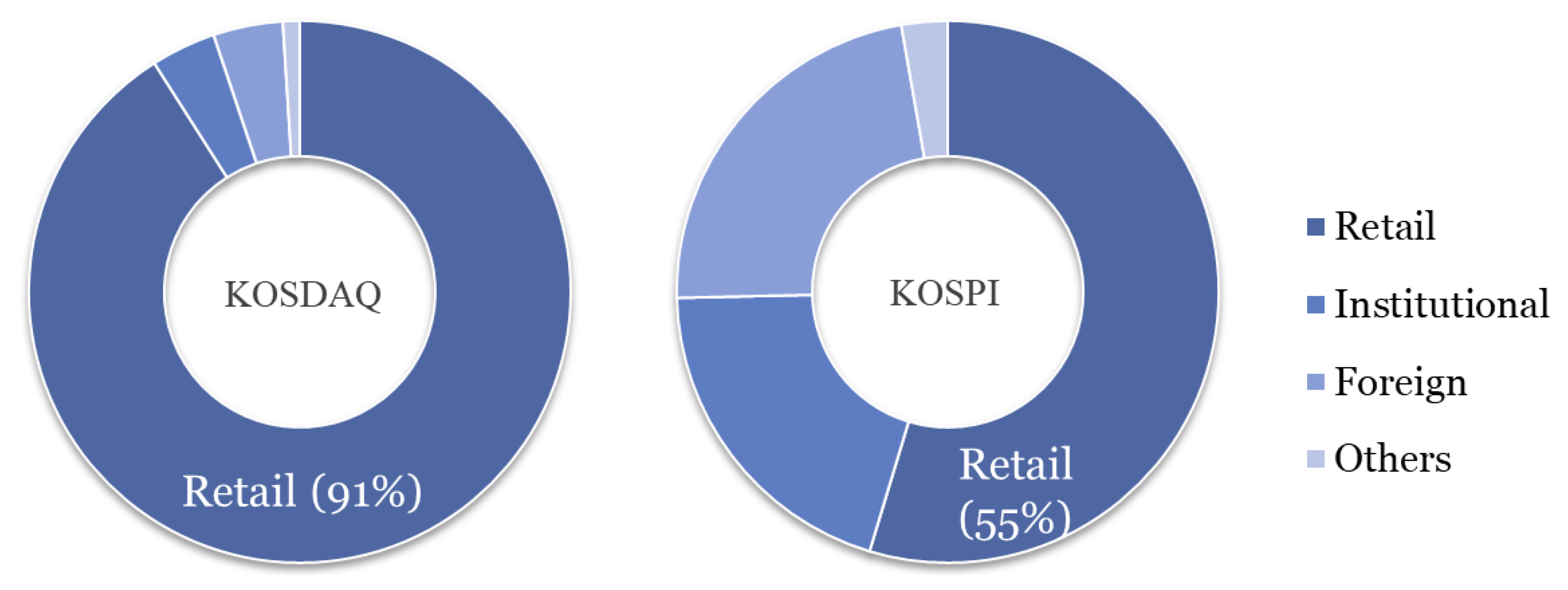
Third, the effect of retail trading on asset prices seemed to be stronger in the KOSDAQ market. While retail trading was more prevalent in the higher-IVOL portfolios for both markets, the overall level of RTP was much higher in the KOSDAQ market, consistent with the earlier market-level evidence. More interestingly, the sign of net trading volume was the opposite of the sign of excess returns in the KOSDAQ market. That is, future returns tended to be positive (negative) for portfolios that individual investors net-sell (net-buy). This evidence also supports our hypothesis that the trading of retail investors affects asset prices, and the influence is stronger on the KOSDAQ market because of the heavy participation of individual investors in this market.
Table 2 shows the future excess returns of IVOL-sorted quintile portfolios for stocks listed on KOSDAQ or KOSPI. At the end of each month, we sorted stocks listed on a market (KOSDAQ or KOSPI) into quintiles based on their IVOLs, estimated using daily data for the one-, three-, or 12-month period prior to the formation date. The results for each estimation window are reported in each panel as indicated. IVOL was computed using the standard deviation of the excess return residuals of the Fama–French three-factor model, where KOSDAQ and KOSPI indices are used as market factors in the KOSDAQ and KOSPI market, respectively. As represented by RET (%), we computed monthly value-weighed (VW) returns in excess of the risk-free rate in the month following the formation date. We define market share as the portion of the market capitalization of a firm or a portfolio in the entire market. SHR is the market share of each portfolio in each investigated market. We constructed quintile portfolios using two break points: (i) Each portfolio should have the same number of stocks or (ii) each portfolio should have equal market shares of 20%.
Table 2 exhibits the two portfolio returns and SHR in each column. At the bottom of each panel, returns on long–short strategies (denoted by 1–5) and their risk-adjusted returns (denoted by FF-
) of the Fama–French three-factor model are reported. To save space, we have only reported the results of the long–short portfolio returns and risk-adjusted returns for the three- and 12-month-windows in Panels B and C. All values are monthly averages during the sample period from January 2001 to December 2017. All t-statistics in parentheses were computed using the Newey and West [
28] corrected standard errors.
Panel A of
Table 2 shows that the cross-sectional relationship between IVOL and future returns was statistically significant and negative in the KOSDAQ market, suggesting that the investment strategy of buying low-IVOL stocks and selling high-IVOL stocks would earn profits. The long–short strategy earned 3.06% per month with a t-statistic of 5.25; it had a corresponding alpha of 2.51% with a t-statistic of 4.29 after adjusting for the Fama–French three risk factors. In contrast, stocks on the KOSPI market did not exhibit such a relationship with statistical significance, which is consistent with our findings in previous studies using KOSPI stocks. The relationship was negative (the Fama–French alpha of the long–short strategy was 0.83% per month) but not statistically significant (t-statistic = 1.27). Panels B and C repeat the same analysis with three- and twelve-month IVOLs, respectively. We have only reported average return and FF-
to save space. The results are qualitatively similar with those in Panel A. Thus, the main finding is not sensitive to the selection of the window length of IVOL estimation.
What creates this difference between the two markets? One sharp contrast is the distribution of market shares of the quintile portfolios. When we constructed portfolios, each of which had an equal number of constituents, the market shares of quintile portfolios in both markets decreased with the size of IVOL. However, the KOSDAQ market had rather similar market values (ranging from 13% to 24%) compared to the KOSPI market where the market share of the highest quintile dropped dramatically (from 35% to 5%). This implies that the negative IVOL-return relation in the KOSPI market might be entirely due to a characteristic of small caps in the 5th quintile portfolio. The last two columns provide further evidence; to control for the effect of that characteristic, we sorted the firms by IVOL again but each portfolio was required to have an equal market share. We see that in the KOSPI market, the negative relation disappears (and even becomes positive); the raw return is −0.48% with a t-statistic of −1.05 and the alpha is 0.19% with a t-statistic of 0.41. In contrast, the statistically significant negative relation remains in the KOSDAQ market after controlling for market share; the magnitude of the profit decreases.
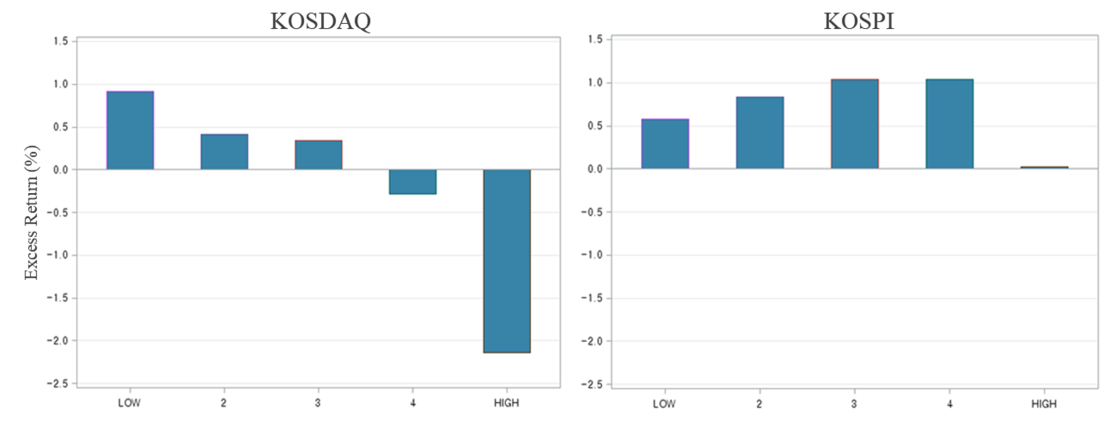
Another distinct feature in the KOSDAQ market is the return pattern across IVOL quintiles. Compared with the KOSPI market, KOSDAQ exhibited a “clearer” negative relation between IVOL and future returns.
Table 2 shows that future excess returns on quintiles exhibited a monotonically decreasing trend with IVOL in KOSDAQ. However, such a pattern was not shown in the KOSPI market; the highest IVOL portfolio earned lower returns than the lowest IVOL portfolio, but average returns increased up to the 4th quintile portfolio. In other words, the IVOL anomaly in KOSPI was merely driven by low returns on the 5th quintile portfolio in which small-cap firms were included. In contrast, the IVOL anomaly in KOSDAQ was more prominent and profitable because the decreasing pattern of returns was present across the entire range of IVOL-sorted portfolios.
Motivated by these findings about the KOSDAQ market, we have examined whether low-volatility investing strategies can be carried out on the KOSDAQ market from the perspective of their risks and profits, in the following sections.
4.2. Profitability of Low-Volatility Investing
We analyzed the profitability of low-volatility investing on the KOSDAQ market with reference to excess returns and risk-adjusted returns.
Table 3 shows the average future returns on the long leg and the short leg and the spread of the long and short legs; the long (short) leg is the lowest (highest) quintile portfolio based on the magnitude of IVOL. An “L/M/N” strategy refers to a trading strategy involving the estimation of IVOL for L months, waiting for M months before investing, and holding portfolios for N months. For example, for a 3/1/1 strategy, we estimate IVOLs using data for three months (L = 3) and wait for one month (M = 1) to avoid market microstructure issues. Then we buy and hold a portfolio for the next month (N = 1). Average future returns were calculated in terms of excess returns (Panel A) or in terms of risk-adjusted returns using the Fama–French three-factor model (Panel B). Both equal-weight (EW) and value-weight (VW) returns are presented. All t-statistics in parentheses were computed using Newey–West corrected standard errors.
In
Table 3, it is worth noting that the long–short strategies generated economically and statistically significant returns in the following month. For example, Panel A of
Table 3 shows that the 12/0/1 strategy yielded the highest VW return of 3.29% (t-statistic = 5.75) and the 1/0/1 strategy yielded the highest EW return of 2.99% per month (t-statistic = 4.98). Panel B of
Table 3 confirms that such profitability remained even after controlling for the Fama–French three factors. The alphas were 2.59% for 12/0/1 (VW) and 2.54% for 1/0/1 (EW) strategies, which were slightly lower than their raw excess return counterparts; statistical significance also dropped slightly, but the 1% significance level remained. While the weighting scheme did not significantly affect the result, VW returns generally earned slightly more. Similarly, the one-month wait was not crucial; by and large, profits declined when we waited for one month before investing regardless of the weighting scheme and the length of the estimation window. Overall, in the KOSDAQ market, a low-volatility investment strategy that buys stocks in the lowest-IVOL quintile and sells stocks in the highest-IVOL quintile can generate statistically significant alphas that are robust to weighting and various L/M/N strategies.
An in-depth analysis into the long and short legs provided more interesting implications. As seen previously, both VW and EW strategies yielded statistically significant future returns. The sources of the profitability, however, differed depending on the weighting scheme. Specifically, average returns on the long (short) leg were statistically significant at the 1–5% level only in the EW (VW) scheme. Moreover, the magnitudes of the returns and the alphas were higher on the long (short) leg for the EW (VW) scheme. This implies that while EW long–short strategies earn most of their profit from the long portfolio, VW long-short strategies earn most of their profit from the short portfolio. These two facts reveal that the source of profits is different for EW and VW strategies.
How can we explain our results? The results of the short leg are not very surprising because they can be explained by the growing corpus of literature on the limits of arbitrage [
22,
29,
30,
31,
32,
33]. The short leg includes stocks with high IVOL. As evidenced by
Table 1, RTP in the short leg was higher than in the long leg, and we hypothesize that this is because retail traders prefer high-IVOL stocks in order to entertain high incomes and overcome limited leverage. The investment amount of retail investors is typically much smaller than that of institutional investors. Also, because of their creditworthiness, retail investors cannot exploit a leverage as much as they want to. Consequently, retail investors have a strong preference for volatility or IVOL. As a result, the short leg is overpriced and subsequently yields negative returns. Even in a competitive and rational market, such abnormal returns can continue to be earned if there exist short-sale constraints. In actuality, it is difficult for short-selling to be carried out by individual investors because of regulations in the KOSDAQ market.
We find the results of the long leg interesting. They are somewhat surprising at two points. First, is it possible for stocks that are “less preferred” by retail investors to be underpriced? In a completely competitive market, a low proportion of unskilled investors means a high proportion of skilled traders. Therefore, if a stock is less preferred by retail investors, it will be correctly priced by skilled traders.
We argue that the high RTP of the KOSDAQ market is the key to the first question. As mentioned earlier, the KOSDAQ market is mainly driven by unskilled retail investors, compared to the KOSPI market; at the market level, the trading volume attributable to foreign and institutional investors—commonly regarded as skilled investors—is very small in the KOSDAQ market. Therefore, low-IVOL stocks that are “less preferred” by retail investors can remain underpriced. As shown in
Table 1, the RTP of stocks in the lowest-IVOL quintile was as high as 82%, although this was lower than the RTP of stocks in the highest-IVOL quintile (97%). In other words, low-IVOL stocks were less preferred by retail investors, which does not necessarily mean that skilled investors correctly priced those stocks. Thus, the “less-preference” of unskilled investors can lead to underpricing in the KOSDAQ market where the influence of individual investor trades cannot be ignored. In
Table 1, the NET values also support our argument. Net buying by retail investors led to negative returns and net selling led to positive returns in the KOSDAQ market, showing opposite signs between NET and RET in all quintiles. This was not found in the KOSPI market where the influence of retail investors was relatively weaker. In unreported results, we confirm that the same phenomenon occurs for decile portfolios.
Second, why do the statistically significant (e.g., at a 1% level) abnormal returns on the long leg persist? Even if low-IVOL stocks can be underpriced, arbitrageurs would exploit the anomaly and the risk-adjusted returns should ultimately be insignificant, both economically and statistically.
Market friction such as trading costs can answer the second question. We argue that trading costs are too high for skilled arbitrageurs to exploit anomaly, and accordingly the KOSDAQ market remains inefficient for several reasons. First, even though the long leg includes large stocks, the total market capitalization of the long leg is only 20 trillion won, which is 0.07 times the long leg of the KOSPI market (approximately 260 trillion won). Second, stocks in the lowest-IVOL quintile (long leg) are more liquid than those in the highest-IVOL quintile (short leg) in KOSDAQ, but they are still illiquid compared to stocks in KOSPI. As measured by Amihud’s illiquidity variable (ILLIQ) in
Table 1, the long leg illiquidity was 12.39 in the KOSDAQ market and 0.25 in the KOSPI market. A large volume of trading would impact prices so significantly that the seemingly profitable anomaly would be unable to generate any profit. Other liquidity measures such as turnover (TURN) and price per share (PRICE) also support our argument that the long leg of KOSDAQ is not attractive to skilled traders with large amounts of funding. Therefore, even if the long leg appears to continue to earn abnormal returns, they are not easily earned because those stocks are small caps, illiquid, and subsequently accompanied by high costs.
4.3. Risks of Low-Volatility Investing
Even if the average returns are highly profitable, asset managers cannot ignore the risks of the portfolios that they manage. We, therefore, now analyze the risks of IVOL trading strategies. Considering that short-only strategies are not common in practice, we have focused on studying long-only and long–short strategies.
The first dimension of risk we have evaluated is maximum drawdown (MDD), the maximum loss of portfolio value in percent during the entire investment period [
34]. If a strategy experiences significant drops in its portfolio value during its term, it is difficult for investors to endure such periods even though the portfolio eventually generates a high return. These significant drops can result in substantial flows of money out of the fund. For this reason, particular attention should be paid to managing a drawdown.
Table 4 shows the MDD for each L/M/N strategy. We found that long–short strategies are less risky than long-only strategies in terms of MDD. For example, while the 1/0/1 EW long-only strategy exhibited an MDD of −50.42%, the MDD of the corresponding long–short strategy was only −32.09%. This means that if an investor invested in this fund, he/she would have experienced a 32.09% loss in money invested during the sample period. While it is true that 32% is not a small loss, considering the fact that the sample period includes a financial crisis during which the KOSDAQ index experienced an MDD of −68.5%, this long–short low-volatility investing strategy can be quite attractive as a defensive strategy.
Another dimension of risk is covariance with existing risk factors such as market, size, and value. A low covariance is preferred because it can provide the advantage of diversification. Covariance is typically estimated by factor loadings (OLS betas). As can be seen in
Table 4, the long-only strategies had a market beta of less than one—ranging from 0.78 to 0.88—depending on weight and L/M/N. Therefore, the long-only low-volatility investing strategy can be a defensive strategy. The long–short portfolio reduced its market beta nearly to zero. In EW cases, it ranged from −0.07 to −0.02; VW cases had a slightly higher exposure, ranging from −0.15 to −0.08. This finding suggests that low-volatility investing can offer a diversification opportunity to mitigate market risk.
Practitioners and academics are also interested in where the premium originates. To investigate the sources of the premiums, we decomposed the profit (average excess return) into four components using the Fama–French three-factor model: The market risk premium (), the size premium (), the value premium (), and an unexplained premium (FF-).
Long-only strategies generally earn their premiums from the alpha, which means that most of the premiums cannot be explained by the Fama–French model. For example, the 1/0/1 EW portfolio earned a premium of 1.74% per month on average, of which 1.28% was alpha. Only 0.46% was due to the three types of risk factors. Among the three sources, the value premium accounted for most of the factor premiums, amounting to 0.42%. Compared to long-only investing, the premiums on the long–short portfolios were far less accounted for by the Fama–French model. Out of the excess return of 2.99%, 2.54% was alpha for the 1/0/1 EW strategy. As with the long-only investing strategy, it was the value premium that accounted for most of the factor premiums. All in all, low-volatility investing has low exposure to traditional risk factors, resulting in a small factor risk premium. Although the factor risk premium is small, the value premium comprises a significant portion of the factor risk premium.
4.4. Robustness Checks
In this section, we test whether our main findings on the profitability of IVOL strategies are robust to a different number of portfolios and to longer holding periods. For the first robustness check, we constructed decile portfolios based on the magnitude of IVOL (in contrast to the quintile portfolios constructed in the main analysis earlier) and repeated the main analysis of
Table 3. The results are presented in
Table 5 and confirm that our main findings in the quintile analysis remain intact even when we sort into deciles. First, the long–short portfolios earned economically and statistically significant profits both in EW and VW schemes. For example, for the 1/0/1 strategy, the EW (VW) profit was 4.15% (4.00%) per month. This was also true for risk-adjusted returns in Panel B, although their magnitudes reduced slightly to 3.59% and 3.33% for EW and VW, respectively. Second, the profit sources of the long–short portfolios were different. Looking at t-statistics, while VW portfolios earned profits from the short leg, EW portfolios earned from the long leg. For the 1/0/1 strategy, for example, the VW short leg had a t-statistic of -4.03, but its long leg showed a t-statistic of 1.39. The opposite argument is true for the EW portfolio. Therefore, we can see that the EW low-volatility strategy earns profits from undervalued stocks, while the VW strategy earns profits from overvalued stocks.
The second robustness check was whether the strategy remained profitable for longer holding periods. In the earlier main analysis, we only investigated profits for one-month holding periods (i.e., strategies with N = 1). We now extended N to examine the returns for three-, six-, and 12-month holding periods. This examination allowed us to not only carry out a robustness check, but to also see how long the profitability persisted.
Table 6 presents the results. We confirm that the profitability remained unchanged when we used holding periods longer than one month. In the earlier result, EW profit was 4.15% for the one month holding period. In
Table 6, the three-, six-, and 12-month holding periods generated 2.27% 2.31%, and 2.04% returns, respectively. Although the economical magnitude reduced as the holding period was extended, we confirm that IVOL investing was still profitable. More interestingly, the profitability persisted for up to 12 months: Both the economical and statistical significance did not weaken over the 12-month holding period. For example, the 1/0/12 excess returns were 2.04% (t = 4.21) and 1.77% (t = 4.38) for the EW and VW portfolios, respectively. These findings are important for practical purposes. In practice, trading costs such as taxes, fees, and bid/ask spreads significantly reduce the net profit. Frequent rebalancing causes higher trading costs and lowers net profit. Some studies have argued that factor investing cannot make profits after considering costs [
35,
36,
37]. Therefore, the finding that low-volatility investing in the KOSDAQ market produces significant profits even for the 12-month holding period implies that trading costs are not a big concern for this investment strategy.


