Dynamic Lifecycle Assessment in Building Construction Projects: Focusing on Embodied Emissions

Abstract

Understanding the structure and behavior of emissions in building systems is the first step toward improving the reliability of the environmental impact assessment of buildings. The shortcomings of current building lifecycle assessment (LCA) research is the lack of understanding of embodied emissions and static analysis. This study presents a methodology for the dynamic LCA of buildings, combined with the system dynamics technique. Dynamic factors related to recurrent embodied emissions are explored through a literature review. Applying the dynamic factors based on the review, a causal map and stock-flow diagram are invented. Collecting the field data and establishing the assumptions based on the literature, a case study is performed for the proposed model. As a result, through dynamic analysis, it was found that recurrent embodied emissions have a considerably different behavior from static ones during their whole life. Additionally, it was found that the environmental impacts changed by more than 10%, according to the variation of the users’ required performance level in sensitivity analysis. This result thoroughly addressed the necessity and appropriateness of dynamic LCA. The dynamic LCA model developed in this study can contribute to the long-term behavioral understanding of the embodied environmental impacts of building LCA.

1. Introduction

Buildings are key factors in energy consumption and global warming, consuming as much as 40% of the resources entering the global economy [1]. Life cycle assessment (LCA), which quantifies the environmental impacts during the whole life of a product, is a useful decision-making tool for green buildings [2]. It has been increasingly used by researchers to assist with decision-making for environment-related strategies and to reduce buildings’ life cycle environmental impacts for the last 25 years [3]. Geng S. et al. [4] reviewed the literature related to building LCA using bibliometrics and showed that the number of publications related to building LCA grew steadily over the past 15 years and more rapidly since 2010.

Additionally, embodied carbon (EC) has recently become especially crucial for estimating the life-cycle carbon of buildings. EC refers to carbon dioxide emitted during the manufacture, transport, and construction of building materials, compared to operational carbon (OC), which means carbon dioxide emitted from the use of buildings, including heating, cooling, and lighting. In a recent review paper by Anand and Amor [5], numerous building LCA studies were explored, and it was shown that the areas of embodied energy had seen the maximum growth in the most recent years. Nevertheless, Pomponi and Moncaster [6] showed an extremely incomplete and short-sighted approach to life cycle studies through their meta-analysis of EC. According to the review, most studies only assess the manufacturing stages, often completely overlooking impacts occurring during the occupancy stage or at the end of life of the building. In other words, carbon emissions from construction and maintenance and repair (M&R) recurring during the building usage have been paid little attention so far. They emphasized that the LCA research community has the responsibility to address such shortcomings and work towards more complete and meaningful assessments. Considering the growing M&R proportion in the contemporary construction industry, embracing recurrent EC caused by M&R intervention activities in building lifecycle must not be overlooked.

Another limitation of LCA is that its analytical method is static. Traditional LCA methods are used to conduct building environmental impact assessment, with little consideration of influential factors that vary in time. Because the lifecycle of a building is quite long, such details have a significant influence on the accuracy of evaluation results [7]. Recently, dynamic LCA (DLCA) studies on buildings were conducted. Collinge [8,9,10,11] built DLCA research and identified significant time-related changes of variables, then developed a dynamic model based on the general LCA equation. Fouquet et al. [12] used a DLCA method to assess the global warming impact of three low-energy houses over time, considering the future electricity mix and innovation of materials for refurbishment. Su et al. [7] developed a dynamic assessment framework based on LCA principles and identified four dynamic building properties.

Previous building DLCA studies have accounted for economic and social progress (e.g., energy mix and Input–Output matrix) and characterization factors (e.g., global warming potential (GWP)). Su et al. [7] have proposed a DLCA framework that considers resident behavioral dynamics. They deal with the dynamic changes, focusing on the operational impacts, but embodied impacts from repair or replacement were not included. Fouquet et al. [12] added the materials used for refurbishment in the dynamic analysis, but they did not reflect the dynamic behavior in the usage stage, only dealing with the differences in the material types themselves. Overcoming the present limitations, this study developed the DLCA model, covering dynamic factors in recurrent embodied impacts in the usage stage and applying the system dynamics.

The objective of the research is to explore the impact of dynamic factors and their interaction with recurrent EC to obtain a better understanding of the recurrent EC in building LCA. This study utilizes system dynamics methodology for DLCA simulation. System dynamics involves the ability to represent and assess the dynamic complexity of the behavior that arises from the interaction of a factors in a system over time [13]. It is an advantageous modeling technique to reflect circular causality in simulation. Since a feedback loop is investigated while searching dynamic factors, system dynamics is considered a highly suitable method for DLCA simulations in this study. Meanwhile, LCA has defined a systematic set of procedures for compiling and examining the inputs and outputs of materials and energy and the associated environmental impacts, directly attributable to the functioning of a product or service system throughout its life cycle [14]. While this study focuses on the usage phase during the whole building life, the systematic process of the LCA principle is used for the equivalent calculation of embodied carbon dioxide in building systems.

The research procedure is as follows. First, dynamic factors related to recurrent EC are discussed in a literature review. According to condition-based management, intervention causing recurrent embodied emissions is determined by the performance. Several factors that impact the building performance are investigated. Second, the DLCA model for recurrent embodied impacts in the usage stage is developed using system dynamics. Applying the dynamic factors based on the review, a causal map and a stock-flow diagram are invented. The causal map is described for the relationship among the dynamic factors. The stock and flow diagram were invented for the DLCA simulation. Third, collecting the field data and establishing the assumptions based on the literature, a case study is performed to validate the proposed model. A base run is performed, with the optimization benchmarking the guideline data, substituted for real data. The base run simulation result, which displays the DLCA, is compared to the static analysis. Sensitivity analysis for embodied recurrent impacts is also performed, varying according to the change of the dynamic factors. This result can address the necessity and appropriateness of DLCA.

2. Literature Review

Most global policy has a tendency to focus on reducing OC since the majority of carbon emissions arise from the building usage [15]. However, recent studies have shown the growing significance of EC because much effort has already been invested into reducing OC [16]. Anand and Amor [5] showed that the research related to embodied energy has been significantly increased in recent years. Gavotsis and Moncaster [15] demonstrates that embodied carbon is also a significant proportion of the whole life impacts from buildings through a detailed case study of a low-energy school building. They also discussed about the uncertainties for post-construction stages. Brown et al. [17] pair attention to significant impacts arising from material production for buildings, and evaluated the importance of EC from refurbishment for operational energy reduction. This study displayed that EC for refurbishment actions take considerable share of the reduction of carbon dioxide emissions achieved by the refurbishment. Dixit [18] conducted a systematic survey of literature to identify parameters specifically affecting the recurrent embodied energy of buildings. It emphasized the need to standardize the parameters and quantify their uncertainties by developing appropriate models. Especially, service life, durability, aesthetics fashion, technology change, tenant change, and functional appropriateness factor, which are strongly related to supplied or required performance of building, were found as parameters affecting the recurrent embodied energy.

Several studies dealing with DLCAs have been recently conducted on the environmental impact of buildings. Negishi et al. [19] identified the time-dependent characteristics of a building system for performing DLCA. In this study, degradation of technical performances of building components, replacement and refurbishment with new technology factors were identified as a part of the key dynamic characteristics of building system. Su et al. [20] formalized four identified dynamic assessment elements in their recent study by examining the data transformation pathway in accordance with the standard LCA framework. Dynamics related to recurrent embodied consumption containing maintenance and demolition were included in the DLCA model.

Su et al. [7] organized dynamic factors in building LCA, classifying them into four categories: technological progress, variation in occupancy, dynamic characteristic factors, and dynamic weighting factors. Dynamic characteristic factors, dynamic weighting factors, and technological progress are related to calculation by the impact category. These factors reflect the variation of social change. The characteristic factors for impact categories could change according to the investigated relative impact for the substance. The weighting factors could vary according to the region, environmental issue, or social trend. Technological progress means the variability of the energy mix, which causes variation in the emission factor value. Variation in occupancy means the variability of the energy consumption behavior. Bringing the variation in the occupancy factor into the embodied sector, it can be expressed as a variation in the intervention behavior. Since this study deals only with the greenhouse effect among the impact categories, dynamic weighting factors are not considered in identifying the dynamic model variables. Moreover, this study primarily explores the factors related to a building itself.

3. Dynamic Factors in Recurrent EC

Since this study focuses on recurrent EC, it is concentrated on the variation in the intervention behavior to explore the dynamic factors. Intervention behavior is a dynamic factor, influenced by the performance of the building. That is, the performance of the building determines the time and amount of intervention. This relationship has been observed in the study of Tarefder & Rahman [21], which developed the lifecycle cost (LCC) model of airport pavement maintenance. In this study, they compared the performance improvement and LCC of the maintenance strategy using two condition indexes of airport pavement, with system dynamics. The initial condition, minimum acceptable condition, condition rise after maintenance, and deterioration were used as model parameters.

The relationship between performance and intervention also appears in existing asset management models. In the US federal facilities portfolios [22], the performance indicators that are used for maintenance decisions are the Facilities Condition Index (FCI) and the Facilities Rehabilitation Rate (FRR). In this model, if the FCI exceeds the acceptable condition level, intervention is applied. The FRR accounts for the required repairs and upgrades. The acceptable condition level will vary according to the mission, agency, organization and importance of specific facilities.

In addition, intervention behavior may differ from the occupants’ characteristic, and likewise, the energy consumption is affected by the occupant behavior in terms of the operational impact. Observing that some home-owners invest heavily in repairs and improvements of their home, but some do not, Leather et al. [23] studied the reason why some occupants delay the maintenance of their home. In their report, different points of view in identifying repair needs, difficulties in finding trustworthy builders, financial problems and several other reasons are revealed as reasons for delayed maintenance. This report clearly showed the effect of occupants’ characteristics on housing maintenance. Additionally, several studied the mentioned users’ tendency to perform maintenance action in mechanical maintenance. Bitan and Meyer [24] examined users’ tendencies to perform preventive maintenance actions. Shavartzon et al. [25] suggested a personalized alert agent for optimal user performance in computing, considering the users’ preferences. It is possible to introduce the occupants’ tendencies to perform the intervention in the housing maintenance field.

As a result of the literature review, dynamic factors to explain the relationship between intervention behavior and performance are identified: (Initial or current) performance, acceptable performance, deterioration, intervention rate, performance rise, and occupant’s tendency. Applying values in a range for the application of several parameters in the existing literature shows the dynamic nature of these factors. This study utilizes these dynamic factors in DLCA modelling.

4. System Dynamics Model for DLCA

4.1. Causal Map and Feedback Loop

In the system dynamics methodology, a system may be represented as a causal map [26]. A causal map is a simple map of a system, with all its constituent components and their interactions. By capturing interactions and feedback loops, a causal map reveals the structure of a system. By understanding the structure of a system, it becomes possible to ascertain a system’s behavior over a certain time period [27].

Since intervention, which causes recurrent embodied carbon during the building usage, strongly depends on the performance of a building, this study invented a causal map, containing the building performance. There is a simple causal relationship among the performance, intervention, and environmental impact. When the performance of a building deteriorates over time, intervention activities, such as repair or replacement, occur. These interventions generate environmental impacts and lead to a performance improvement. Thus, the performance of the building is recovered. If the building is in a sufficiently good condition, the intervention activity does not occur, and the environmental impact also does not occur. Without intervention for a while, the performance of the building is degraded again, and intervention activities occur again. This process will continue to be repeated during the life of buildings. This relationship is shown in the causal map below (Figure 1).

Especially, the causal map showed the feedback loop among the performance, performance improvement, and intervention. Combining the positive and negative relationships between the variables, the causal map has a negative feedback loop (balancing loop). This means that an increase of a parameter in the feedback loop consequently caused a decrease of itself. For example, a performance increase engenders zero or less intervention, and an intervention decrease causes a performance decrease. This balancing feedback loop suggests that the embodied environmental impact of the usage phase will converge, instead of diverting upward or downward.

Figure 2 displays the causal relationship in the initial construction and intervention. The typical environmental impact calculation process is also presented. The environmental impact is affected by the quantity of construction activity and emission factors, which are calculated by multiples of them. Additionally, recurring environmental impacts from intervention during the usage phase is influenced by the initial construction, because the quantity of materials and activities of intervention is likely to be determined based on the initial one.

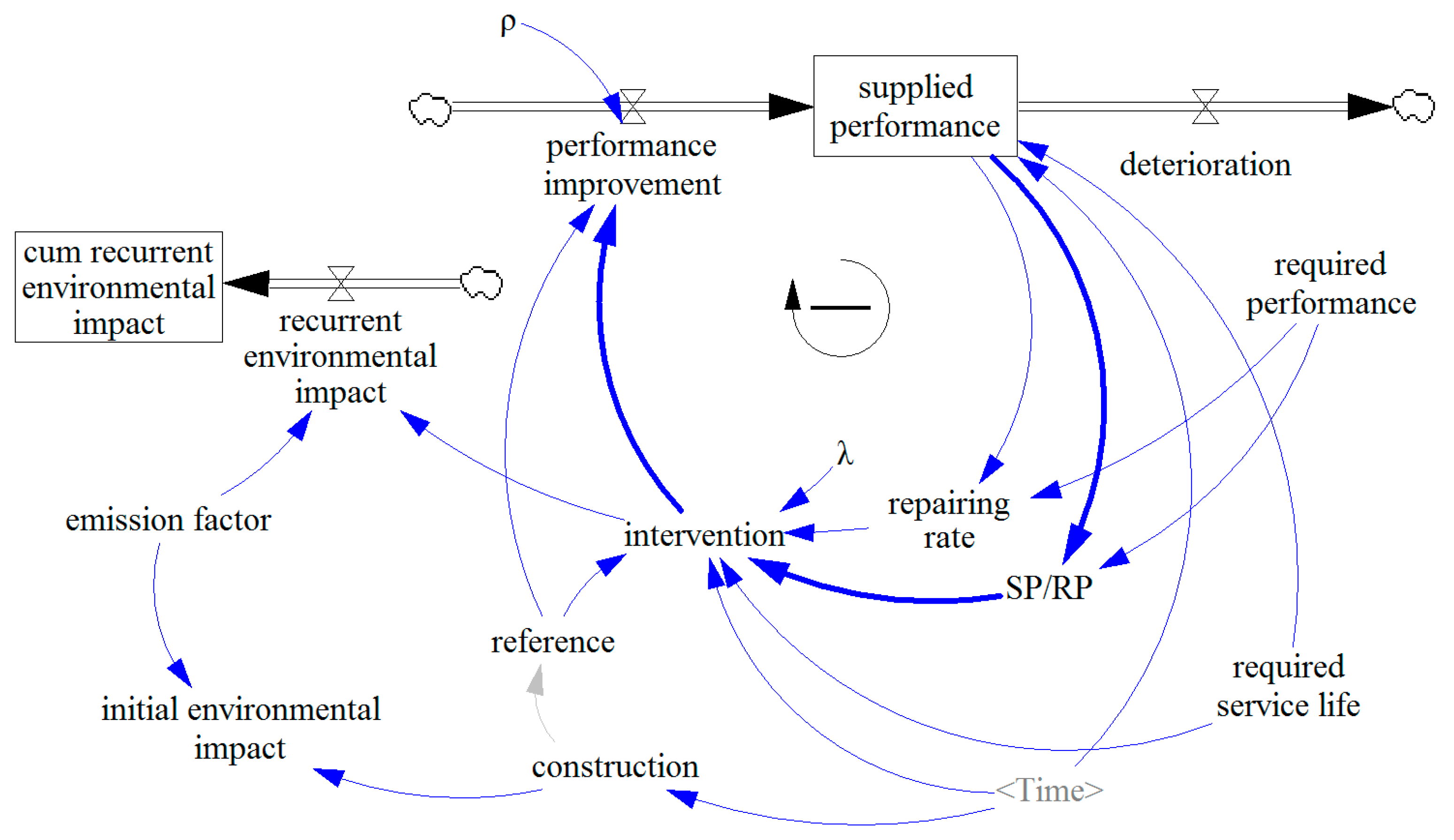
4.2. Stock and Flow Diagram (SFD)

To perform a more detailed quantitative analysis, a causal map is transformed into an SFD. A stock and flow model aids in the study and analysis of the system in a quantitative way. A stock is the term for any entity that accumulates or depletes over time. A flow is the rate of change in a stock.

Considering the invented causal map, which contains the feedback loop, SFD was developed. In this process, additional parameters are required to answer several questions for the quantitative model: (1) When should intervention activities be applied? (2) How much intervention should be applied? (3) How will performance be improved by intervention activities?

(1) When should intervention activities be applied: ratio of supplied performance (SP) to required performance (RP), and maintenance of strategy strength.

Studies that estimate the existing M&R-related embodied environmental impacts are based on several guidelines that provide the durability of construction materials. The guidelines are based on ‘InterNACHI’s estimated life expectancy chart [28]’ and the ‘Study of life expectancy of home components’ [29]. Previously, the material life expectancy was provided by the experimental data under the daily conditions, and the latter provides a value based on the data surveyed by the manufacturer. The purpose of these guidelines is mainly to provide a lifetime warranty of home components for residents. Many respondents noted that this lifetime is variable in terms of maintenance levels and emphasized that the lifetime of the component is changed before consumers are satisfied [30]. However, previous studies have deterministically decided the timing of interventions based on a guideline with a fixed lifecycle.

This study deals with the intervention times, as a variable that is determined by the performance. The intervention activity will occur when the supplied performance is lower than the required performance. Executing repair or replacement, the supplied performance can be improved to a level that satisfies the required performance. Therefore, this study uses the ratio of supplied performance to the required performance (SP/RP) as a parameter. If the value is greater than 1, the supply performance is good. If the value is less than 1, the supply performance does not satisfy the required performance.

In addition to the ratio of the supplied performance to the demand performance, this study introduces a parameter that can represent the maintenance strategy strength (λ). The occupants or building managers may want to prevent falling below the required performance through proactive maintenance, although the SP/RP is greater than 1. On the other hand, even if the SP/RP is less than 1, the building may not require immediate intervention to save maintenance costs or for other reasons, unless it is physically dangerous. λ is a parameter representing this occupants’ tendency. If λ is greater than 1, a preemptive strategy is adopted. If λ is less than or equal to 1, a cost-effective strategy is adopted. Intervention is performed when SP/RP becomes smaller than λ, as shown below.

IF THEN ELSE (“SP/RP” < λ, intervention, 0))

(2) How much intervention should be applied: repairing rate.

According to the Multi-Family Housing Management Act in Korea, the repairing rate is defined as a percentage of the cost of repairs for unpredictable partial damage or failure of a specific part of a building. The Enforcement Decree of the Multi-Family Housing Management Act in Korea proposed the repairing cycle and the repairing rate for each component in the ‘Guidelines for a long-term repair program’. These guidelines propose what repairing cost is charged for fixed repairing periods for establishing long-term repairing plans.

The concept of this repairing rate can be used to estimate the extent of repair. The original rate is used to estimate the repairing cost, but in this study, it is used to estimate the quantity. In assessing environmental impacts, the volume of the material is the key factor that determines the amount of activity involved. The intervention quantity can be defined as the product of the initial construction quantity and the repairing rate, as shown below.

intervention = initial construction × repairing rate

As the repair time varies according to the supplied performance and the required performance of the building, the repairing quantity will also be variably determined, depending on the performance of the period. In this study, the repairing rate is defined as the ratio of the required performance to the gap between the repairing performance and the supplied performance, as shown in the following. Combined with the definitions mentioned above, the final repairing time and quantity are defined as follows.

repairing rate = (RP − SP)/RP
IF THEN ELSE (“SP/RP” < λ, initial construction × repairing rate, 0))

(3) The extent to which the performance will be improved by intervention activities: ratio of intervention quantity to initial construction.

When intervention activities are performed, performance is improved. Performance improvement will increase the supplied performance of buildings and meet the required performance. The question is the extent to which the performance improvement is created by the intervention activity. As a result of investigating the asset management tools of the US federal agencies [22], indices are developed to accumulate and predict information about the supplied performance, the amount of intervention, and the timing of intervention. However, quantitative indicators of performance improvement by intervention are not found. This may be because the asset management or facility management deals with the building condition, focusing on the budget expenditure.

Quantitative indicators representing the degree of performance improvement are not utilized in the present asset management and facility management fields. It could be intuitively deduced that the performance improvement due to intervention is proportional to the amount of intervention. In this study, it is intended to quantify the performance improvement by introducing a coefficient (ρ) that can represent a proportional relationship according to this intuition.

performance improvement = (intervention/initial construction) × ρ

The above definition is based on the assumption that the performance improvement is simply proportional to only the intervention ratio, compared to the initial construction quantity. ρ is a coefficient indicating the relation between intervention quantity ratio and function improvement. Here, ρ is a coefficient, with a yet unknown value. This value could be found through a model calibration in a further case study.

The SFD was created by adding the introduced variables, described above, and setting the stock and flow variable. The supplied performance is determined according to the stock variable, where the performance deterioration is the outflow variable, and the performance improvement is the inflow variable. In addition, the cumulative recurrent environmental impact is added as a stock variable to identify the total amount of recurrent environmental impacts during the building service life. The model includes the required service life parameter of the building, so that there is no intervention activity when the required service life is reached. The reference variable is a parameter generated for the calculation to refer to the initial construction value throughout the analysis period and does not affect the relationship between the variables in the environmental impact system of the usage stage. The SFD is shown in Figure 3. The bold arrows represent the feedback loop, analyzed in the causal map.

5. Case Study

5.1. Data Information

The case building is a 30-story apartment building, with a reinforced concrete structure. This building consists of five types of floor plans, with a floor area of 146.48 m², 158.89 m², 161.25 m², 161.75 m², and 272.8 m², accommodating 117 generations. A summary of the building construction and the bill of quantity (BoQ) were collected for the building.

Referencing the existing research [31,32] that thoroughly analyzed the target materials of the Korean apartment building for LCA, this study determines the main materials for the case study: Rebar, ready-mixed concrete, concrete brick, cement, insulations, and paints are selected. However, existing studies tend to overlook the materials that are used in the finishing work, probably because of their lightweight and fewer emissions, comparing the structural components by cut-off rules. Since this study focuses on the intervention activities, some non-structural materials, which are repaired or replaced during the building usage, need to be considered. In this context, board, tile, granite, wallpaper, and flooring are also selected.

Using the National lifecycle inventory database by KEITI [33] and KICT [34], Greenhouse Gases (GHGs) emission factors are calculated. Three types of GHGs, carbon dioxide, methane, and nitrous oxide are considered among the lots of GHGs, considering the GWP and its importance, according to the IPCC report.

Table 1. Main materials and emission factors.

Item	Unit	Emission Factors (kgCO2eq/Unit)	Reference
High tensile rebar	kg	3.962 × 10−1	KICT
Ready-mixed concrete, 25-210-12	m3	4.001 × 102	KEITI
Ready-mixed concrete, 25-240-15	m3	4.196 × 102	KEITI
Concrete brick	kg	1.222 × 10−4	KICT
Cement	ton	1.049 × 103	KEITI
EPS foam	kg	2.024	KICT
Tile	kg	3.454 × 10−1	KICT
Granite	kg	4.421	KEITI
Gypsum board	kg	1.383 × 10−1	KEITI
Mineral wool board	kg	1.482	KEITI
Paint, Water-soluble emulsion type	ton	3.089 × 102	KEITI
Paint, Amino-alkyd type	ton	7.833 × 102	KEITI
Paint, Epoxy type	ton	3.158 × 103	KEITI
MDF flooring	EA	1.844	KICT
PVC wallpaper	m2	1.953	KICT

EA (each) = 1.2 × 0.19 × 0.01 m³ (size of one MDF flooring panel).

below shows the selected main materials and respective emission factors used in the case study.

5.2. Assumptions in the Case Study

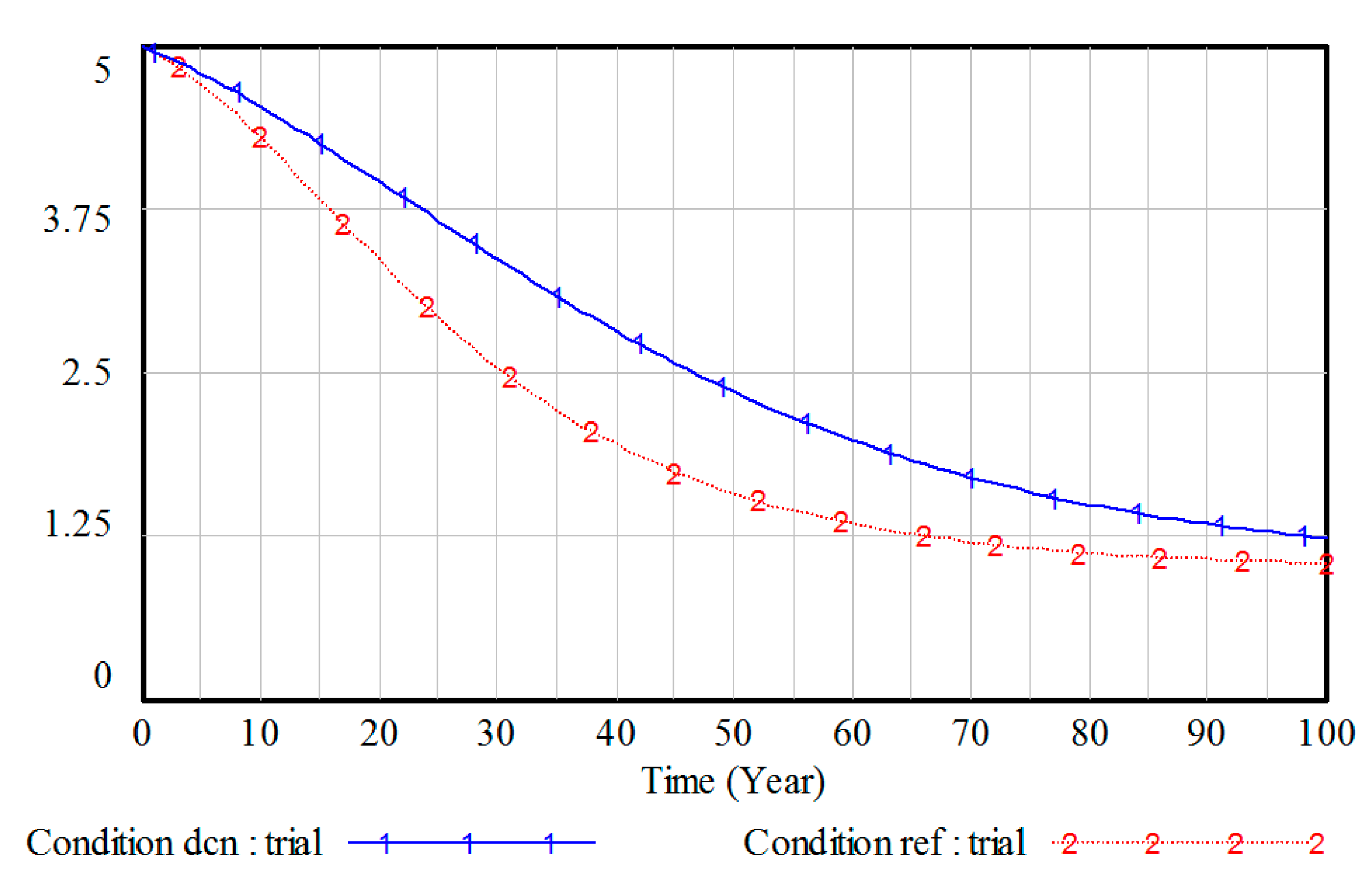
In EN 15978 [35], the system boundary for assessment is described, and the assessment modules in the building lifecycle are defined, as shown in Figure 4. Among the assessment modules, A1–A3 in the product stage, A4 and A5 in the construction process stage, B2–B5 in the usage stage, and C1–C4 in the end-of-life stage are relevant to the embodied impact (faded part in Figure 4). Since the DLCA model is focused on the recurrent EC, the case study is performed within modules B2–B5. The carbon emissions in modules A1–A5 were also calculated ahead of the simulation, because several variables in the DLCA model refer to initial construction information.

This study introduced several assumptions in the case study due to the availability of data.

Table 2. Assumptions of the case study.

Case Study	Variables	Assumption
LCA	Transportation	Delivery distance is assumed to be 20 km for every material.
	Lifting	Allocation rules with lifting weight are applied to common equipment (tower crane, construction lift).
	Carriage-on-site	While they are emission sources, they are not accounted for.
	M&R activities	While they are emission sources, they are not accounted for.
Simulation	Performance	Performance is quantified in a five-point scale.
	Deterioration	Deterioration curve refer to the existing literature [37].
	M&R history	M&R history data are assumed from the guidelines of the Enforcement Decree of the Multi-Family Housing Management Act.

shows the assumptions applied in the emissions calculation, with an LCA and Dynamic simulation.

Building embodied emissions are caused by two factors, material use (the energy consumption in production) and construction activities (the energy consumption by transportation and execution). Material type and quantity data are quite well found in BoQ or the standard unit cost book. However, activity data, such as transportation or carriage-on-site, are not easy to obtain, since they are not well documented during construction. Moreover, M&R activity data, such as the type of repair machinery, work time, and productivity, are even harder to acquire, compared with new construction. Consequently, even if several activities cause carbon emissions, they are excluded from the calculation.

Meanwhile, several variables applied in SFD for dynamic simulation do not allow the real data to be acquired. M&R history data, such as the repair method, time, and quantity in relation to private buildings, are not yet recorded and organized in a database. Accordingly, the guidelines from Enforcement Decree of the Multi-Family Housing Management Act in Korea are assumed. Performance is quantified in a five-point scale, based on the condition grading system for building assets in the International Infrastructure Management Manual [36]. Additionally, there is no system for the performance assessment of private buildings, so deterioration (performance history) data are virtually assumed, referencing the existing study [37].

Keshavarzrad et al. [37] presented deterioration curves using the National Asset Management Support data. They used the Markov model for the prediction of the deterioration trend. A Markov chain has been used in deterioration prediction in relation to bridges [38] and sewers [39]. Sharabah [40] introduced a weighting model for building assemblies using Markov process data, collected from Victorian city councils. Edirisinghe et al. [41] also applied the Markov model for building deterioration prediction.

The state transition probabilities and deterioration curves might be different for each building component. Components using materials with short service lives will have a high probability of transitioning to the next state (curve 2), and components using durable materials will have a significantly higher probability of staying current than transitioning to the next state (curve 1). Since a well-founded transition matrix that can be referred to in the literature is limited, two types of condition curves are virtually adopted. Figure 5 shows the two types of condition curves, resulting from the Markov model calculation. Stone work and interior finishing work, which recommend a repair time of more than 25 years in the guidelines, are applied to deterioration data form curve 1, assuming their performance is relatively slowly degraded. The plastering, tiling, painting and decoration works are applied data from curve 2.

5.3. Simulation

Ideal data for the model calibration of this study would be the actual repair or replacement details, collected for the apartment building. In particular, information, such as the repair time, type of repair activity, and quantity of repair, is required for each object. However, there is still a lack of data accumulation on the repair content of buildings. Therefore, the guidelines in the Housing Act is applied, instead of the real-world value for the calibration of the model. Despite the fact that the guidelines of the Housing Act do not match the real world, calibration based on this reference means reflecting a long-term repair documentary plan in Korean apartment housing.

Comparing carbon emissions and cumulative carbon emissions during the building service life, based on the repairing time and rate from the Housing Act guidelines, λ, ρ, and the required performance parameters are optimized. Initial running with an initial λ = 0.9, the initial performance = 4 is simulated for the model variables for the 50-year study period. Optimized λ, ρ, and the required performance value from the calibration, with a payoff, is displayed in

Table 3. Optimized λ, ρ, and the required performance from the calibration.

Elements	λ	ρ	Required Performance	Simulations (Times)	Payoff
M-RO	0.90	14.40	4.01	490	−1.70 × 108
M-IF	0.90	14.85	4.00	661	−2.67 × 109
T-RO	0.90	35.12	4.06	652	−2.52 × 104
T-IW	1.20	35.41	4.01	833	−6.80 × 1010
T-IF	0.90	148.87	4.16	734	−1.19 × 107
S-EW	0.93	50.00	4.05	632	−1.20 × 109
I-IC	0.93	10.00	4.00	444	−3.30 × 108
I-IW	0.91	1.00	4.30	469	−2.95 × 109
P-EW	1.17	8.45	4.00	562	−4.80 × 108
P-IC	1.20	8.44	4.39	660	−1.14 × 107
P-IW	1.17	8.45	4.00	562	−8.97 × 107
P-ST	1.17	8.48	4.00	456	−1.25 × 104
D-IF	0.90	21.01	3.99	732	−1.40 × 1012
D-IW	0.90	19.18	4.00	438	−3.38 × 1010

M = plastering; T = tile; S = stone; I = interior finishing; P = painting; D = decoration; RO = roof; EW = exterior wall; IC = interior ceiling; IW = interior wall; IF = interior floor; ST = stair.

.

A base run with the parameters’ input value from the calibration results is simulated. The total embodied GHG emissions are 1.97 million kgCO_2eq in the dynamic model (Base run), whereas they are 1.528 million kgCO_2eq in the static calculation from the Housing Act guidelines (Figure 6).

Despite the optimization, the difference between the model and the guidelines is considerable. The dynamic model tends to have a lower intervention than the guideline value, at the beginning of the building service life, and this becomes more frequent as the building ages. Additionally, the intervention quantity is small at the beginning and grows larger at the end of the building’s life in the dynamic model. While the static calculation shows a periodic value, ignoring the building condition, the dynamic model can describe the changing period and quantity of the intervention. Regardless of the benchmark data reality, this conceptual method presents the specific tool for dynamic LCA. It also shows the possibility of anticipating a realistic intervention and its environmental impact in advance.

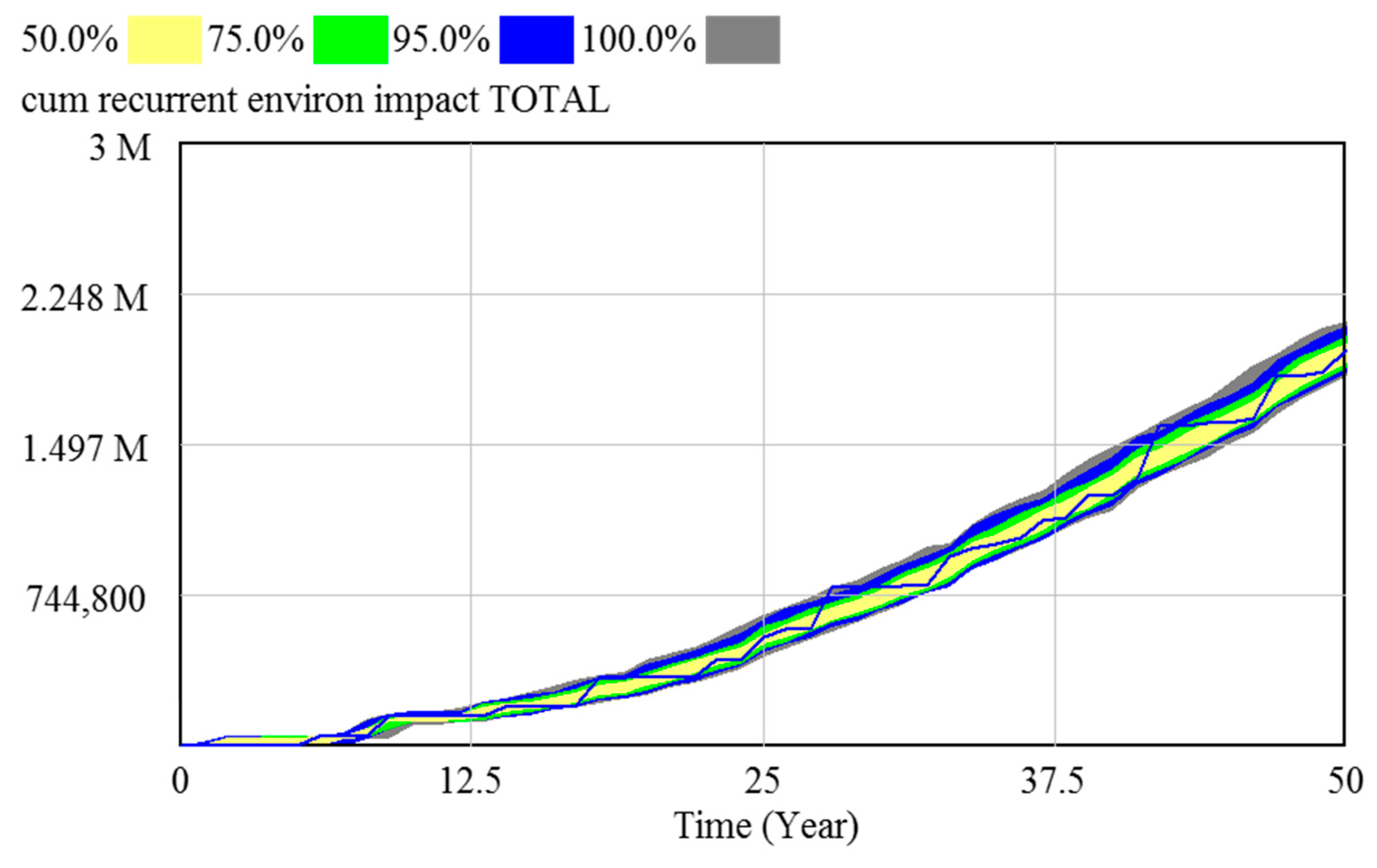
5.4. Sensitivity Analysis

Using the developed dynamic model with a calibrated base run allows for an analysis of the variability involved in the environmental impact of construction activity in the usage stage. In this study, sensitivity analysis is performed on the variability of environmental impacts using two parameters. First, we analyzed the λ, which shows the intensity of the maintenance strategy. The λ variability of the sensitivity analysis was set to ±10% of the values derived from each trade and object in the calibration (

Table 4. Sensitivity analysis results concerning the maintenance strategy intensity (λ).

	λ		GHGs Emission (kgCO2eq)
Component	Min	Max	Min	Max	Stdev	(Max-Min)/Avg
M-RO	0.81	0.99	14,188	15,085	320	6.1%
M-IF	0.81	0.99	55,720	60,821	1417	8.8%
T-RO	0.81	0.99	168	201	11	17.6%
T-IW	1.08	1.32	94,314	94,314	0	0.0%
T-IF	0.81	0.99	4453	6881	991	44.4%
S-EW	0.84	1.03	16,762	43,086	7296	101.8%
I-IC	0.84	1.03	18,331	18,331	0	0.0%
I-IW	0.82	1.00	44,641	44,641	0	0.0%
P-EW	1.05	1.28	26,235	26,235	0	0.0%
P-IC	1.08	1.32	4039	4039	0	0.0%
P-IW	1.05	1.28	35,845	35,845	0	0.0%
P-ST	1.05	1.29	134	134	0	0.0%
D-IF	0.81	0.99	1,417,770	1,600,330	52,475	12.5%
D-IW	0.81	0.99	195720	195,720	0	0.0%
Total	-	-	1,930,130	2,140,150	53,182	10.6%

). Sensitivity analysis applies the Monte Carlo simulation method, which generates random numbers, according to the probability distribution. Since we do not know about the specific probability distributions for λ, a simply uniform distribution was assumed. The analysis results are shown in Figure 7. With λ changes, the total embodied emissions in the usage stage from the base run of 1970 tCO_2eq could range from at least 1930 tCO_2eq to 2140 tCO_2eq.

In other words, each λ variation of 20% resulted in a total embodied emissions value, in the usage stage variation, of approximately 10.6%. The variation ratio of the embodied emissions for each trade and object in accordance with the λ variation is described in Table 4. There were several components that did not change, regardless of the λ variation, tile work in the interior wall, interior finishing work in the interior ceiling and wall, painting work in every object, and decoration work in the interior wall. Stone work is the most sensitive work affected by λ, even if it occupies a small percentage in the total emissions. Tile work in the interior floor, tile work in the roof, decoration work in the interior floor, plastering work in the interior floor, and plastering work in the roof were found to have a high sensitivity in sequence.

Next, the sensitivity is analyzed for the required performance of the building users. The required performance variation was ±10% of the values derived from each trade and object in the calibration in the sensitivity analysis (

Table 5. Sensitivity analysis results concerning the required performance.

	Required Performance		GHGs Emission (kgCO2eq)
Component	Min	Max	Min	Max	Stdev	(Max-Min)/Avg
M-RO	3.61	4.42	13,733	15,344	425	11.2%
M-IF	3.60	4.40	54,868	61,930	1644	12.3%
T-RO	3.66	4.47	169	227	14	31.1%
T-IW	3.61	4.41	75,569	139,221	14,571	64.7%
T-IF	3.75	4.58	2929	7154	1074	97.6%
S-EW	3.65	4.46	20,787	20,787	0	0.0%
I-IC	3.60	4.40	18,331	18,331	0	0.0%
I-IW	3.87	4.73	44,641	44,641	0	0.0%
P-EW	3.60	4.40	26,235	26,235	0	0.0%
P-IC	3.95	4.83	4039	4039	0	0.0%
P-IW	3.60	4.40	35,845	35,845	0	0.0%
P-ST	3.60	4.40	134	134	0	0.0%
D-IF	3.59	4.39	1,357,820	1,622,000	62,445	18.1%
D-IW	3.60	4.40	195,720	195,720	0	0.0%
Total	-	-	1,848,360	2,111,350	61,997	13.4%

). The specific probability distribution of the required performance is also unknown, so a uniform distribution is assumed for the Monte Carlo simulation. The analysis results are shown in Figure 8. As the required performance changes, the total embodied emissions in the usage stage, from 1970 tCO_2eq in the base run, can vary from at least 1848 tCO_2eq to 2111 tCO_2eq.

Each required performance variation of 20% resulted in the embodied emission variation of approximately 13.4% during the usage stage. The variation ratio of the embodied emissions for each trade and object, in accordance with the required performance variation, is described in Table 5. There were several components that did not change, regardless of the required performance, stone work, interior finishing work in the interior ceiling and wall, painting work in every object, and decoration work in the interior wall. Tile work in the interior floor is the most sensitive work affected by the required performance, even if it occupies a small percentage of the total emissions. Tile work in the interior wall, tile work in the roof, decoration work in the interior floor, plastering work in the interior floor, and plastering work in the roof were found to have a high sensitivity in sequence.

Under the same conditions, the required performance was found to be more sensitive to changes in emissions for the components and total value than λ. The rate of change in tile work tends to have the largest ratio, and the painting work shows no change for both λ and the required performance. Stone work was the most sensitive work in terms of λ but did not show any variation in the required performance.

Adding a larger amount of data accumulation and elaborate assumptions, this analysis can be a useful tool for preliminarily verifying the variability of the repair scenarios for each trade and object. In addition, the evaluation of the life cycle environmental impacts, taking into account the variability of the intervention scenarios, could be useful for risk analysis in building environmental management.

6. Conclusions

Maintenance activities mainly depend on changes in building performance over time, but the static methodology of traditional LCA does not take this variability into account. Besides, current embodied environmental impact assessment has tended to focus on the structural materials, and decorating materials used in M&R are overlooked. This study combines system dynamics with LCA to assess the recurrent embodied carbon emissions. It visualizes the long-term behavior of the environmental impacts caused by the feedback structure between the building performance and intervention. Additionally, the variability of the environmental impacts, from the changes in users’ required performance and maintenance strategy intensity, is analyzed.

The results of this study show the possibility of acquiring a great amount of important information that could not be captured by the traditional LCA methodology. It shows how the estimates of environmental impacts, assuming the application of fixed repair cycles and ratios, differ from the actual performance-based maintenance concept. This implies that it is possible to provide statistical information on the uncertainty of the forecast when estimating the emissions, and it can support the reliability of the environmental impact estimation of buildings.

This study has some limitations in terms of data collection and utilization. First, because the site of the case building was closed, it was impossible to collect activity data on the building. A simulation was performed using assumptions and data from the literature, and analysis based on the measured data should be performed in the next study. A lot of activity data, generated in M&R work during the usage stage, are not accessible and difficult to measure. Nevertheless, data acquisition for several sample works would be a meaningful starting place, before considering whole buildings.

Additionally, because of the lack of available information about performance degradation, it was replaced with data from the existing study. While the main interest of this study is the relationship between the building performance and the environmental impact, the accuracy of the deterioration data is important in the model, since performance is a major variable determining the timing of M&R. It is necessary to explore the performance deterioration, which is suitable for the LCA target building, through the accumulation of performance evaluation for representative buildings.

References

1. Ji, C.; Hong, T.; Jeong, J.; Kim, J.; Lee, M.; Jeong, K. Establishing environmental benchmarks to determine the environmental performance of elementary school buildings using LCA. Energy Build. 2016, 127, 818–829. [Google Scholar] [CrossRef]
2. Zuo, J.; Pullen, S.; Rameezdeen, R.; Bennetts, H.; Wang, Y.; Mao, G.; Zhou, Z.; Du, H.; Duan, H. Green building evaluation from a life-cycle perspective in Australia: A critical review. Renew. Sustain. Energy Rev. 2017, 70, 358–368. [Google Scholar] [CrossRef]
3. Atmaca, A. Life cycle assessment and cost analysis of residential buildings in south east of Turkey: Part 1—Review and methodology. Int. J. Life Cycle Assess. 2016, 21, 831–846. [Google Scholar] [CrossRef]
4. Geng, S.; Wang, Y.; Zuo, J.; Zhou, Z.; Du, H.; Mao, G. Building life cycle assessment research: A review by bibliometric analysis. Renew. Sustain. Energy Rev. 2017, 76, 176–184. [Google Scholar] [CrossRef]
5. Anand, C.K.; Amor, B. Recent developments, future challenges and new research directions in LCA of buildings: A critical review. Renew. Sustain. Energy Rev. 2017, 67, 408–416. [Google Scholar] [CrossRef]
6. Pomponi, F.; Moncaster, A. Embodied carbon mitigation and reduction in the built environment—What does the evidence say? J. Environ. Manag. 2016, 181, 687–700. [Google Scholar] [CrossRef] [PubMed]
7. Su, S.; Li, X.; Zhu, Y.; Lin, B. Dynamic LCA framework for environmental impact assessment of buildings. Energy Build. 2017, 149, 310–320. [Google Scholar] [CrossRef]
8. Collinge, W.O.; Liao, L.; Xu, H. Enabling dynamic life cycle assessment of buildings with wireless sensor networks. In Proceedings of the 2011 IEEE International Symposium on Sustainable Systems and Technology, Chicago, IL, USA, 16–18 May 2011; pp. 1–6. [Google Scholar]
9. Collinge, W.; Landis, A.E.; Jones, A.K.; Schaefer, L.A.; Bilec, M.M. Indoor environmental quality in a dynamic life cycle assessment framework for whole buildings: Focus on human health chemical impacts. Build. Environ. 2013, 62, 182–190. [Google Scholar] [CrossRef]
10. Collinge, W.O.; Landis, A.E.; Jones, A.K.; Schaefer, L.A.; Bilec, M.M. Dynamic life cycle assessment: Framework and application to an institutional building. Int. J. Life Cycle Assess. 2013, 18, 538–552. [Google Scholar] [CrossRef]
11. Collinge, W.O.; Landis, A.E.; Jones, A.K.; Schaefer, L.A.; Bilec, M.M. Productivity metrics in dynamic LCA for whole buildings: Using a post-occupancy evaluation of energy and indoor environmental quality tradeoffs. Build. Environ. 2014, 83, 339–348. [Google Scholar] [CrossRef]
12. Fouquet, M.; Levasseur, A.; Margni, M. Methodological challenges and developments in LCA of low energy buildings: Application to biogenic carbon and global warming assessment. Build. Environ. 2015, 90, 51–59. [Google Scholar] [CrossRef]
13. Rahim, F.H.A.; Hawari, N.N.; Abidin, N.Z. Supply and demand of rice in Malaysia: A system dynamics approach. Int. J Sup. Chain. Mgt. 2017, 6, 1–7. [Google Scholar]
14. ISO 14040:2006 Environmental Management-Life Cycle Assessment-Principles and Framework. Available online: https://www.iso.org/standard/37456.html (accessed on 8 July 2019).
15. Gavotsis, E.; Moncaster, A. Improved embodied energy and carbon accounting: recommendations for industry and policy. Athens J. Tech. Eng. 2015, 2, 9–23. [Google Scholar] [CrossRef]
16. Kang, G.; Kim, T.; Kim, Y.W.; Cho, H.; Kang, K.I. Statistical analysis of embodied carbon emission for building construction. Energy Build. 2015, 105, 326–333. [Google Scholar] [CrossRef]
17. Brown, N.W.O.; Olsson, S.; Malmqvist, T. Embodied greenhouse gas emissions from refurbishment of residential building stock to achieve a 50% operational energy reduction. Build. Environ. 2014, 79, 46–56. [Google Scholar] [CrossRef]
18. Dixit, M.K. Life cycle recurrent embodied energy calculation of buildings: A. review. J. Clean. Prod. 2019, 209, 731–754. [Google Scholar] [CrossRef]
19. Negishi, K.; Tiruta-Barna, L.; Schiopu, N.; Lebert, A.; Chevalier, J. An operational methodology for applying dynamic Life Cycle Assessment to buildings. Build. Environ. 2018, 144, 611–621. [Google Scholar] [CrossRef]
20. Su, S.; Li, X.; Zhu, Y. Dynamic assessment elements and their prospective solutions in dynamic life cycle assessment of buildings. Build. Environ. 2019, 158, 248–259. [Google Scholar] [CrossRef]
21. Tarefder, R.A.; Rahman, M.M. Development of system dynamic approaches to airport pavements maintenance. J. Transp. Eng. 2016, 142, 04016027. [Google Scholar] [CrossRef]
22. Davis, J.S.; Cable, J.H. Key Performance Indicators for Federal Facilities Portfolios, Federal Facilities Council Technical Report Number 147; The National Academies Press: Washington, DC, USA, 2005. [Google Scholar]
23. Leather, P.; Littlewood, M.; Munro, M. Home-Owners and Housing Repair: Behavior and Attitudes; Joseph Rowntree Foundation (JRF): York, UK, 1998. [Google Scholar]
24. Bitan, Y.; Meyer, J. Self-initiated and respondent actions in a simulated control task. Ergonomics 2007, 50, 763–788. [Google Scholar] [CrossRef]
25. Shavartzon, A.; Azaria, A.; Kraus, S.; Goldman, C.V.; Meyer, J.; Tsimhoni, O. Personalized alert agent for optimal user performance. In Proceedings of the Thirtieth AAAI Conference on Artificial Intelligence, Phoenix, AZ, USA, 12–17 February 2016. [Google Scholar]
26. Sterman, J.D. Business Dynamics: Systems Thinking and Modeling for a Complex World; McGraw: New York, NY, USA, 2000. [Google Scholar]
27. Meadows, D. Thinking in Systems: A Primer; Earthscan: London, UK, 2008. [Google Scholar]
28. International Association of Certified Home Inspectors (InterNACHI). InterNACHI’s Standard Estimated Life Expectancy Chart for Home. Available online: https://www.nachi.org/life-expectancy.htm (accessed on 15 May 2019).
29. Seiders, D.; Ahluwalia, G.; Melman, S.; Quint, R.; Chaluvadi, A.; Liang, M.; Silverberg, A.; Bechler, C.; Jackson, J. Study of Life Expectancy of Home Components; National Association of Home Builders (NAHB), Bank of America (BoA) Home Equity: Washington, DC, USA, 2007. [Google Scholar]
30. Seiders, K.; Voss, G.B.; Godfrey, A.L.; Grewal, D. SERVCON: Development and validation of a multi-dimensional service convenience scale. J. Acad. Mark. Sci. 2007, 35, 144–156. [Google Scholar] [CrossRef]
31. Shin, S.; Tae, S.; Woo, J.; Roh, S. The development of environmental load evaluation system of a standard Korean apartment house. Renew. Sustain. Energy Rev. 2011, 15, 1239–1249. [Google Scholar] [CrossRef]
32. Choi, D.S.; Chun, H.C.; Ahn, J.Y. Prediction of Environmental Load Emissions from an Apartment House of Construction Phase through the Selection of Major Materials. J. Archit. Inst. Korea Plan. Des. 2012, 28, 237–246. [Google Scholar]
33. Korea Environmental Industry & Technology Institute (KEITI). Korea Life Cycle Inventory Database. 2004. Available online: http://www.epd.or.kr/lci/lciDb.do (accessed on 15 May 2019).
34. Korea Institute of Civil Engineering and Building Technology. The Final Report of National DB on Environmental Information of Building Materials; KICT: Goyang, Korea, 2008. [Google Scholar]
35. EN 15978:2011 Sustainability of construction works-Assessment of the environmental performance of buildings-Calculation methods. Available online: https://shop.bsigroup.com/ProductDetail?pid=000000000030256638 (accessed on 8th July 2019).
36. IPWEA. International Infrastructure Management Manual. Available online: https://www.ipwea.org/publications/ipweabookshop/iimm (accessed on 8th July 2019).
37. Keshavarzrad, P.; Setunge, S.; Zhang, G. Deterioration prediction of building components. In Proceedings of the 2014 Sustainability in Public Works Conference, Tweed Heads, Australia, 27–29 July 2014; pp. 1–9. [Google Scholar]
38. Madanat, S.; Mishanlani, R.; Ibrahim, W.H.W. Estimation of infrastructure transition probabilities from condition rating data. J. Infrastruct. Syst. 1995, 19, 120–125. [Google Scholar] [CrossRef]
39. Baik, H.S.; Jeong, H.S.; Abraham, D.M. Estimating Transition Probabilities in Markov Chain-Based Deterioration Models for Management of Wastewater Systems. J. Water Resour. Plan. Manag. 2006, 132, 15–24. [Google Scholar] [CrossRef]
40. Sharabah, A.; Setunge, S.; Zeephongsekul, P. A Reliability Based Approach for Service Life Modeling of Council Owned Infrastructure Assets. In Proceedings of the ICOMS Asset Management Conference, Melbourne, Australia, 22–25 May 2007. [Google Scholar]
41. Edirisinghe, R.; Setunge, S.; Zhang, G. Markov Model-Based Building Deterioration Prediction and ISO Factor Analysis for Building Management. J. Manag. Eng. 2015, 31, 04015009. [Google Scholar] [CrossRef]
Figure 1. Causal map of building performance and environmental impact.
Sustainability 11 03724 g001
Figure 2. Causal map of construction activity and environmental impact.
Sustainability 11 03724 g002
Figure 3. Stock and Flow Diagram of environmental impact in building usage stage.
Sustainability 11 03724 g003
Figure 4. System boundary and assessment modules in building lifecycle assessment.
Sustainability 11 03724 g004
Figure 5. Condition curve of reference and discretion.
Sustainability 11 03724 g005
Figure 6. Comparison of the base run and Housing Act in the Greenhouse Gases of the usage stage.
Sustainability 11 03724 g006
Figure 7. Sensitivity analysis results on maintenance strategy intensity (λ).
Sustainability 11 03724 g007
Figure 8. Sensitivity analysis results concerning the required performance.
Sustainability 11 03724 g008