A Bayesian Network-Based Integrated for Flood Risk Assessment (InFRA)


Abstract
:1. Introduction
2. Materials and Theories
2.1. Existing Flood Risk Assessment Indices
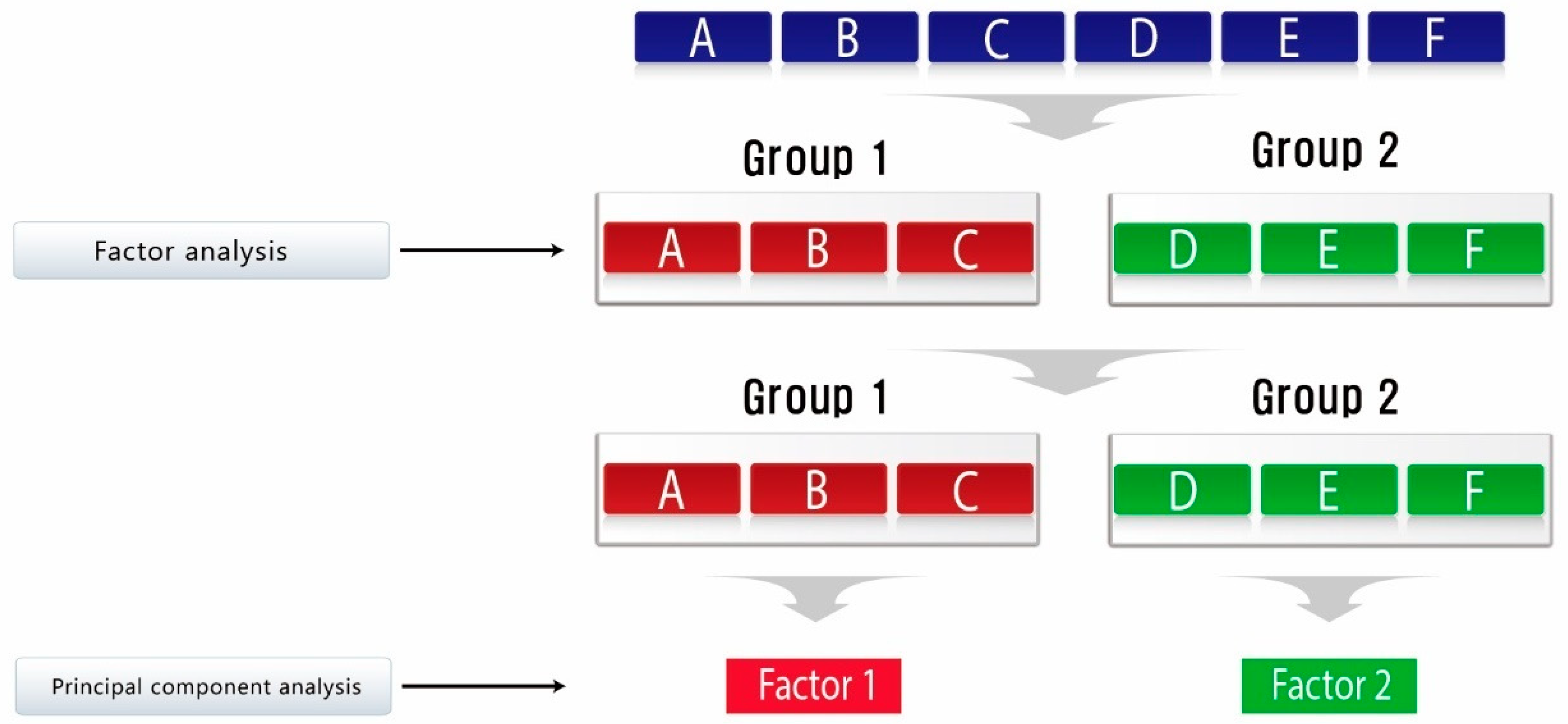
2.2. Methodology for Selecting Representative Indicators
2.3. Methodology for Assigning Weights
- (1)
- Matrix construction
- (2)
- Normalization of assessment items
- (3)
- Calculation of entropy of each attribute
- (4)
- Weight assignment between assessments
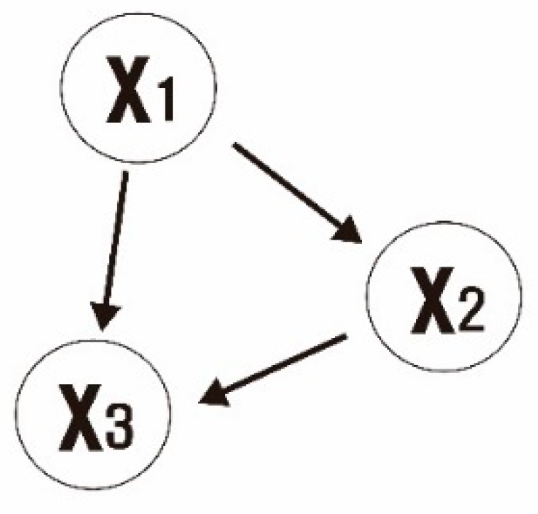
2.4. Bayesian Networks (BNs)
2.5. Integrated Index for Flood Risk Assessment (InFRA)
- = hydro-geology
- = socio-economics
- = climate
- = flood protection and
- = weight of each indicator
- = each indicator
- = the weights of each indicator
3. Application and Results
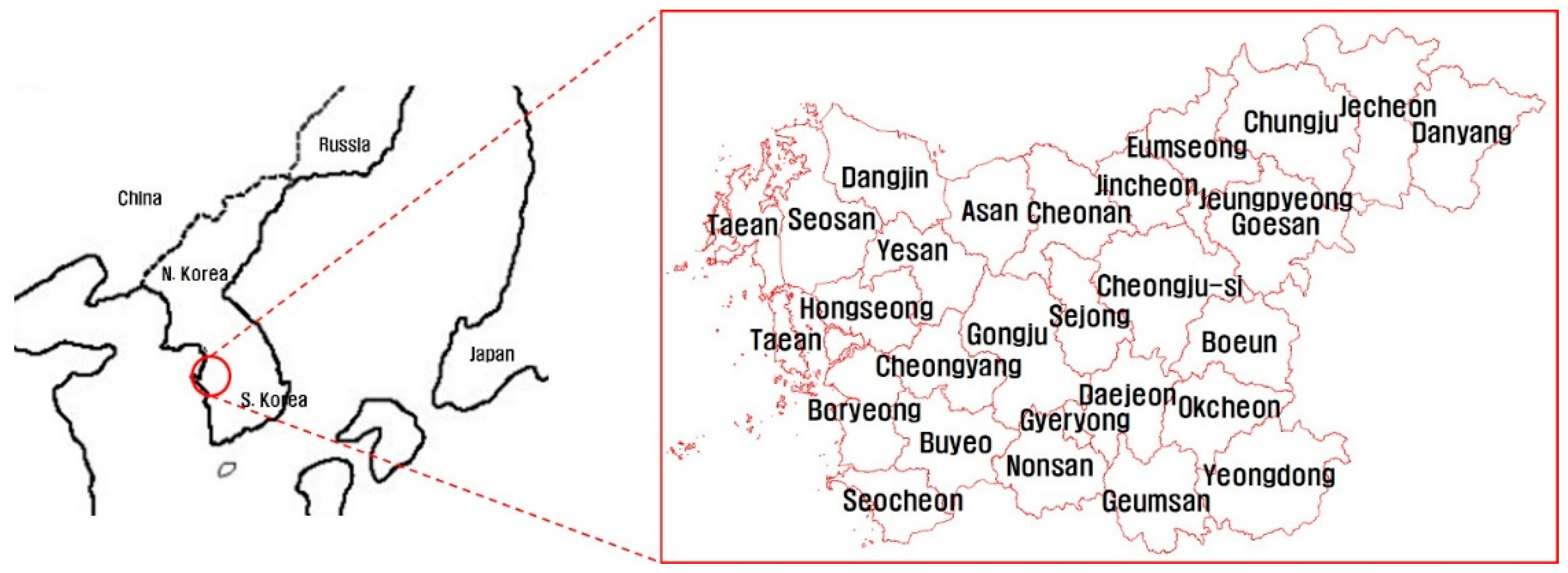
3.1. Selection of Target Areas and Data Collection
3.2. Selection of Indicators Using Factor Analysis and Principal Component Analysis
3.3. Weight Assignment by Method and Calculation of Integrated Weights
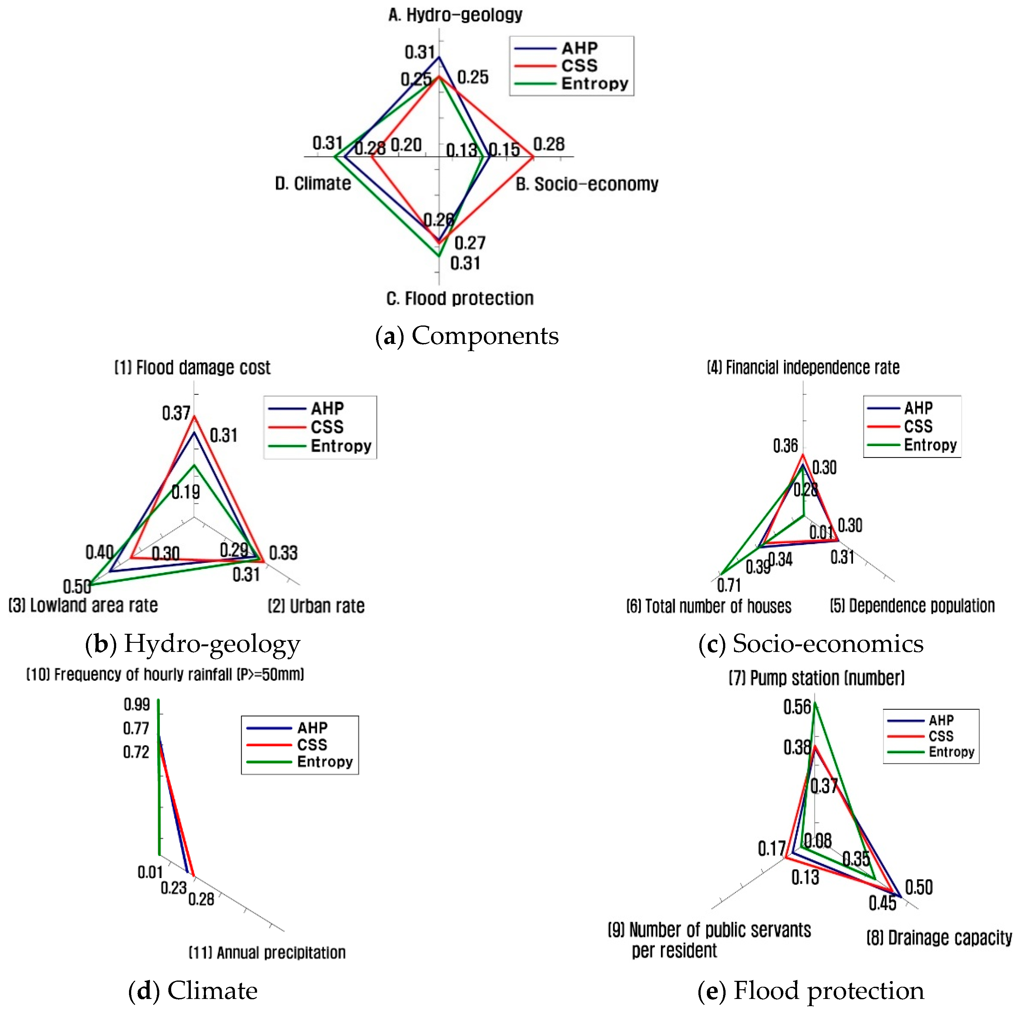
3.3.1. Weight Assignment by Method
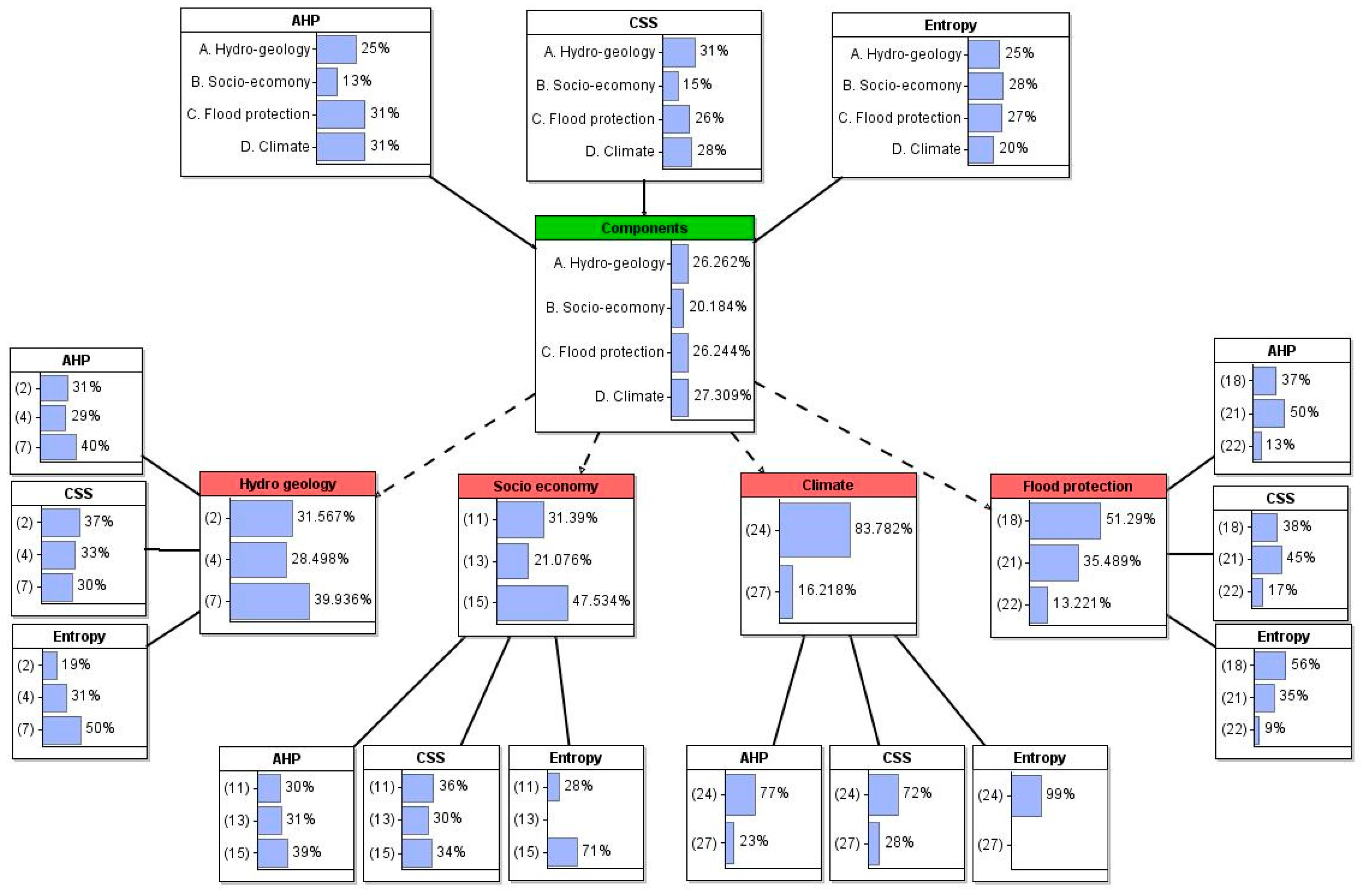
3.3.2. Integrated Weight Assignment Using Bayesian Networks (BNs)
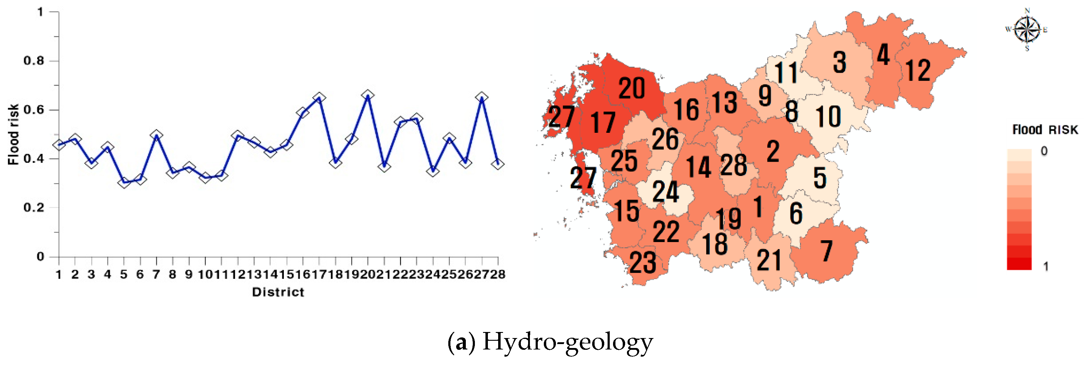
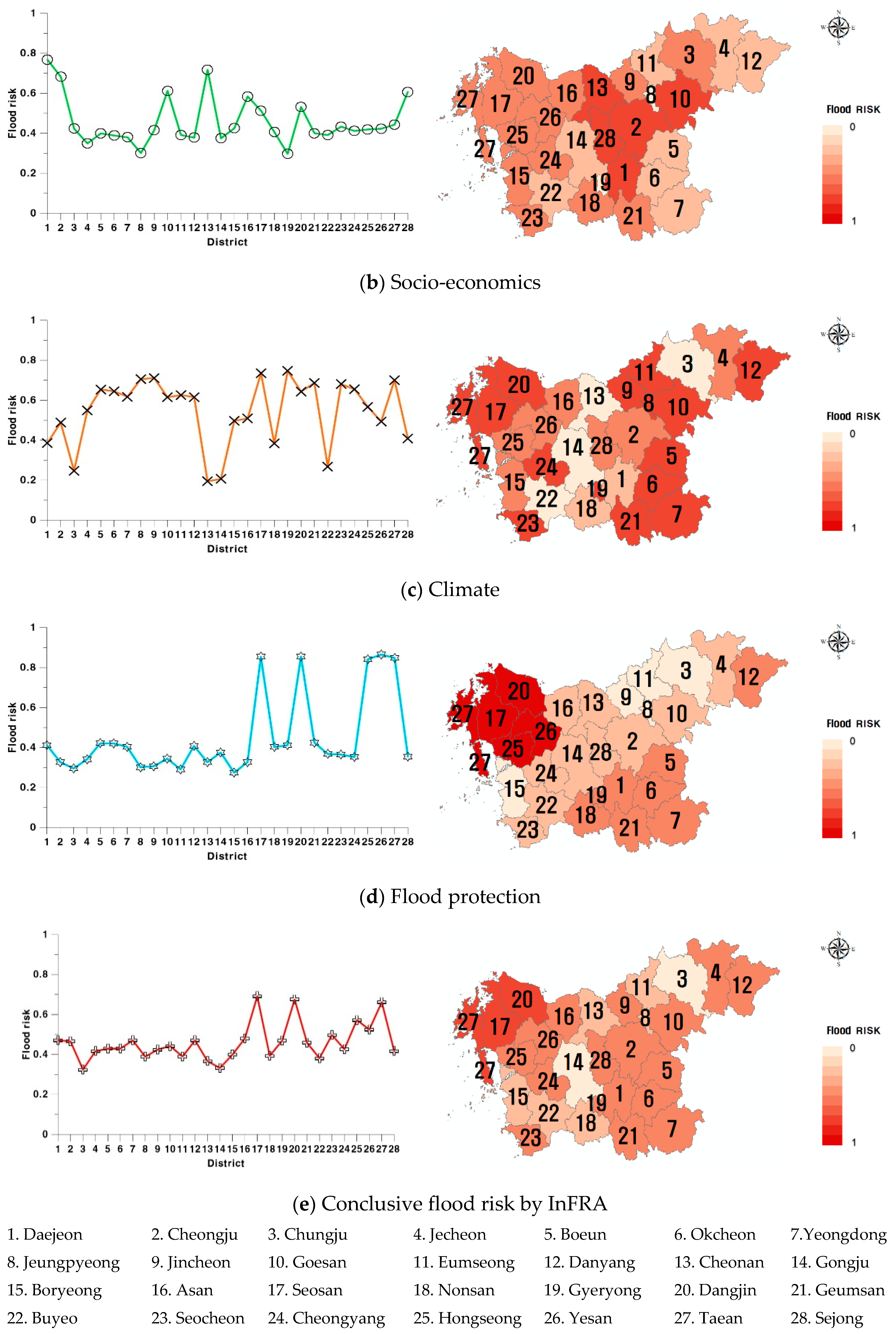
3.4. Results of Calculation with InFRA
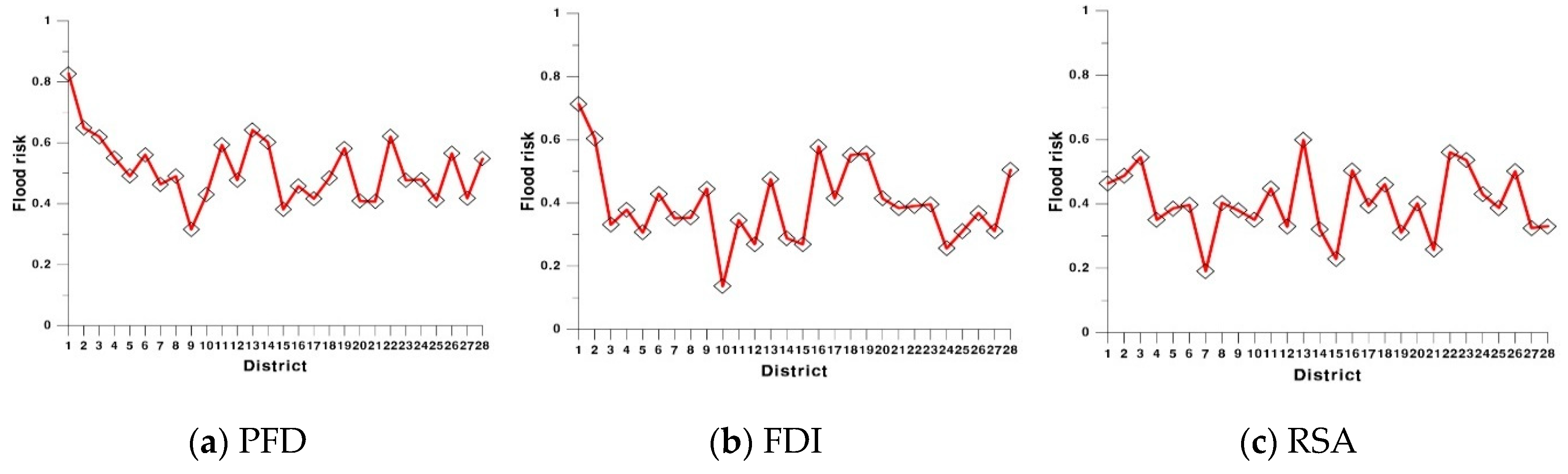
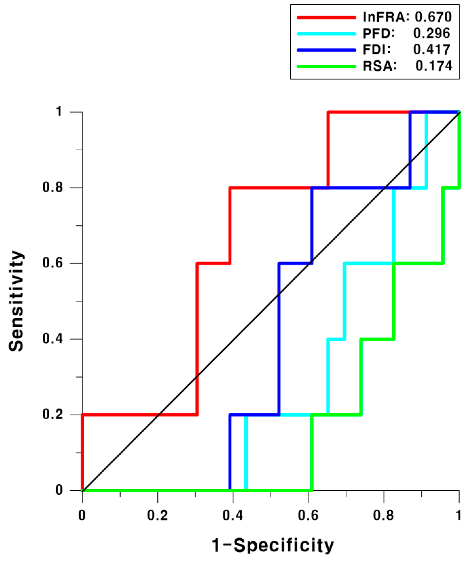
3.5. Comparison with Other Methods and Discussion
4. Conclusions
Author Contributions
Funding
Conflicts of Interest
References
- Luo, P.; Mu, D.; Xue, H.; Duc, T.N.; Dinh, K.D.; Takara, K.; Nover, D.; Schladow, S.G. Flood inundation assessment for the Hanoi Central Area, Vietnam under historical and extreme rainfall conditions. Sci. Rep. (Nat.) 2018, 8, 12623. [Google Scholar] [CrossRef] [PubMed]
- Luo, P.; He, B.; Takara, K.; Xiong, Y.E.; Nover, D.; Duan, W.; Fukushi, K. Historical Assessment of Chinese and Japanese Flood Management Policies and Implications for Managing Future Floods. Environ. Sci. Policy 2015, 48, 265–277. [Google Scholar] [CrossRef]
- Federal Emergency Management Agency. Flood Information Tool User Manual (Rev. 7); FEMA: Washington, DC, USA, 2003.
- National Oceanic and Atmospheric Administration. Risk Vulnerability Assessment Tool; NOAA: Washington, DC, USA, 2007.
- Annual Report 2004: Advancing Innovation; Munich Re Group: München, Germany, 2004.
- Tyndall Centre. Vulnerability, Risk and Adaptation: A Conceptual Framework, Tyndall Centre for Climate Change Research; Tyndall Centre: Norwich, Norfolk, UK, 2003. [Google Scholar]
- Rygel, L.; O’Sullivan, D.; Yarnal, B. A method for constructing a social vulnerability index: An application to hurricane storm surges in a developed country. Mitig. Adapt. Strateg. Glob. Chang. 2006, 11, 741–764. [Google Scholar] [CrossRef]
- Chang, L.F.; Huang, S.L. Assessing urban flooding vulnerability with an emergy approach. Landsc. Urban Plan 2015, 143, 11–24. [Google Scholar] [CrossRef]
- Kablan, M.K.A.; Dongo, K.; Coulibaly, M. Assessment of social vulnerability to flood in urban Côte d’Ivoire using the MOVE Framework. Water 2017, 9, 292. [Google Scholar] [CrossRef]
- Luo, P.; Zhou, M.; Deng, H.; Lyu, J.; Cao, W.; Takara, K.; Nover, D.; Schladow, S.G. Impact of forest maintenance on water shortages: Hydrologic modeling and effects of climate change. Sci. Total Environ. 2018, 615, 1355–1363. [Google Scholar] [CrossRef] [PubMed]
- Luo, P.; He, B.; Duan, W.; Takara, K.; Nover, D. Impact assessment of rainfall scenarios and land-use change on hydrologic response using synthetic Area IDF curves. J. Flood Risk Manag. 2015, 11, S84–S97. [Google Scholar] [CrossRef]
- Environment Agency. Catchment Flood Management Plans: CFMP Guidelines Volume 1 Consultant Report; EA: Almondsbury, Bristol, UK, 2004.
- Jeollabuk-do Total Human Institute National of Korea. Improv. Flood Plans Against Clim. Chang. Jeollabuk-do 2010, 107, 1415–1419.
- Korea Institute of Civil Engineering and Building Technology. Strengthen Facility Standards Against Excess Climate; KICT: Ilsan, Gyeonggi, Korea, 2009. [Google Scholar]
- Korea Research Institute for Human Settlements. Analysis of Flood Damage Characteristics and Development of Flood Damage Index; KRIHS: Sejong, Korea, 2005. [Google Scholar]
- Korea Environment Institute. Development and Introduction of Indicators to Assess Vulnerability of Climate Change; KEI: Sejong, Korea, 2008.
- Ministry of Land, Transport and Maritime Affairs. National Water Resource Plan; MOLTMA: Sejong, Korea, 2001.
- Ministry of Land, Transport and Maritime Affairs. National Water Resource Plan (2010–2020); MOLTMA: Sejong, Korea, 2010.
- National Disaster Management Research Institute. Development of Assessment System for Flood Vulnerability Index; NDMI: Ulsan, Korea, 2012.
- National Institute for Land and Infrastructure Management. Flood Vulnerability Index; NIMIL: Tsukuba, Asahi, Japan, 2009.
- Seoul Institute. Development of the Regional Safety Assessment Model in Seoul–Focusing on Flood; SI: Seoul, Korea, 2006. [Google Scholar]
- World Meteorological Organization (WMO). Guide to Hydrological Practices, 5th ed.; WMO: Geneva, Switzerland, 2008. [Google Scholar]
- Rummel, R.J. Applied Factor Analysis, 1st ed.; Northwestern University: Illinois, IL, USA, 1988. [Google Scholar]
- Shlens, J. A Tutorial on Principal Component Analysis. Cornell Univ. 2014, 1404, 1101. [Google Scholar]
- Fischhoff, B. Value elicitation: Is there anything in there. Am. Psychol. 1991, 46, 835–847. [Google Scholar] [CrossRef]
- Keeny, R.L.; von Winterfeldt, D.V.; Eppel, T. Eliciting public values for complex policy decisions. Manag. Sci. 1990, 36, 1011–1030. [Google Scholar] [CrossRef]
- Joo, H.J.; Kim, S.J.; Lee, M.J.; Kim, H.S. A study on determination of investment priority of flood control considering flood vulnerability. J. Korean Soc. Hazard Mitig. 2017, 18, 417–429. [Google Scholar] [CrossRef]
- Saaty, R.W. The Analytic Hierarchy Process–What It Is and How It Is Used. Math. Model. 1987, 9, 161–176. [Google Scholar] [CrossRef]
- Dudek, F.J.; Baker, K.E. The constant method applied to scaling subjective dimensions. Am. J. Psychol. 1956, 69, 616–624. [Google Scholar] [CrossRef] [PubMed]
- Ozkul, S.; Harmancioglu, N.B.; Singh, V.P. Entropy-based assessment of water quality monitoring networks. J. Hydrol. Eng. 2000, 5, 90–100. [Google Scholar] [CrossRef]
- Jensen, F.V. An Introduction to Bayesian Networks; Springer: New York, NY, USA, 1966. [Google Scholar]
- Kim, S.J.; Rarhi, P.; Jun, H.D.; Lee, J.H. Evaluation of drought severity with a Bayesian network analysis of multiple drought indices. J. Water Resour. Manag. 2017, 144, 1–10. [Google Scholar] [CrossRef]
- Pearl, J. Probabilistic Reasoning in Intelligent Systems: Networks of Plausible Inference; Elsevier: San Francisco, CA, USA, 2014. [Google Scholar]
- Kaiser, H.F. An index of factorial simplicity. Psychometrika 1974, 39, 31–36. [Google Scholar] [CrossRef]
- Bartlett, M.S. Properties of sufficiency and statistical tests. Proc. R. Soc. Lond. Ser. A 1937, 160, 268–282. [Google Scholar]
- Castelletti, A.; Soncini-Sessa, R. Bayesian networks and participatory modelling in water resource management. Environ. Model. Softw. 2007, 22, 1075–1088. [Google Scholar] [CrossRef]
- Henriksen, H.J.; Barlebo, H.C. Reflections on the use of Bayesian belief networks for adaptive management. J. Environ. Manag. 2008, 88, 1025–1036. [Google Scholar] [CrossRef] [PubMed]
- Ministry of the Interior and Safety. Natural Disaster Investigation and Recovery Planning Guidelines; MOIS: Sejong, Korea, 2017.


| Classification | MOLTMA | NDMI | JTHINK | KRIHS | SI | ||
|---|---|---|---|---|---|---|---|
| Components | Indicators | EFVI | PFD | FDRRI | FVA | FDI | RSA |
| A. Hydro-geology | (1) Flood hazard area | ○ | ○ | ||||
| (2) Flood damage cost for public facilities | ○ | ○ | ○ | ○ | ○ | ||
| (3) Imperviousness | ○ | ○ | ○ | ○ | |||
| (4) Urban rate | ○ | ||||||
| (5) Curve number (CN) | ○ | ||||||
| (6) Basin slope | ○ | ○ | ○ | ||||
| (7) Lowland area rate | ○ | ○ | |||||
| (8) Stream density | ○ | ||||||
| B. Socio-economy | (9) Population density | ○ | ○ | ○ | ○ | ||
| (10) Asset (reference land price) | ○ | ○ | ○ | ||||
| (11) Financial independence rate | ○ | ○ | ○ | ○ | |||
| (12) Infrastructure | ○ | ○ | ○ | ||||
| (13) Dependence population | ○ | ○ | |||||
| (14) Manufacturing output in value | ○ | ||||||
| (15) Total number of houses | ○ | ||||||
| C. Climate | (16) Frequency of hourly rainfall (P ≥ 50 mm) | ○ | ○ | ||||
| (17) Frequency of intensive rainfall per day (P ≥ 150 mm) | ○ | ○ | |||||
| (18) Maximum hourly rainfall | ○ | ||||||
| (19) Annual precipitation | ○ | ||||||
| (20) Probability rainfall | ○ | ||||||
| D. Flood Protection | (21) Levee maintenance | ○ | ○ | ||||
| (22) Levee length | ○ | ○ | |||||
| (23) Pump station (number) | ○ | ||||||
| (24) Pump station (capacity) | ○ | ||||||
| (25) Dam and reservoir | ○ | ||||||
| (26) Drainage capacity | |||||||
| (27) Number of public servants per resident | ○ | ||||||
| (28) Index of damage reduction ability | ○ | ○ | |||||
| Classification | Component Points (Selected: ◎) | Eigenvalue | KMO | Barlett’s Test of Sphericity | |||||||||
|---|---|---|---|---|---|---|---|---|---|---|---|---|---|
| Comp-Onents | Indic-Ators | Group | Factor | Chi-Square | df(p) | ||||||||
| 1 | 2 | 3 | 1 | 2 | 3 | ||||||||
| 1. Hydro-geology | (1) | 0.420 | −0.168 | 0.751 | 4.43 | 1.96 | 1.34 | 0.75 | 128.3 | 36(0) | |||
| (2) | −0.479 | −0.518 | 0.951 | ○ | |||||||||
| (3) | 0.351 | 0.674 | 0.055 | ||||||||||
| (4) | −0.229 | 0.895 | ○ | −0.092 | |||||||||
| (5) | 0.658 | 0.096 | −0.080 | ||||||||||
| (6) | −0.237 | −0.172 | 0.378 | ||||||||||
| (7) | 0.850 | ○ | −0.096 | −0.042 | |||||||||
| (8) | −0.333 | 0.124 | 0.627 | ||||||||||
| 2. Socio-economy | (9) | 0.764 | 0.286 | 0.198 | 4.35 | 1.54 | 1.01 | 0.67 | 164.7 | 21(0) | |||
| (10) | 0.694 | 0.088 | 0.001 | ||||||||||
| (11) | 0.147 | 0.957 | ○ | 0.237 | |||||||||
| (12) | 0.595 | 0.216 | 0.150 | ||||||||||
| (13) | −0.412 | −0.326 | 0.523 | ○ | |||||||||
| (14) | 0.144 | 0.351 | 0.010 | ||||||||||
| (15) | 0.902 | ○ | 0.354 | 0.158 | |||||||||
| 3. Climate | (16) | 0.827 | ○ | −0.018 | - | 2.30 | 1.18 | - | 0.65 | 27.2 | 10(0) | ||
| (17) | −0.572 | 0.580 | |||||||||||
| (18) | 0.628 | −0.500 | |||||||||||
| (19) | 0.108 | 0.903 | ○ | ||||||||||
| (20) | −0.342 | 0.776 | |||||||||||
| 4. Flood protection | (21) | 0.802 | −0.030 | −0.32 | 2.87 | 1.46 | 1.25 | 0.54 | 78.7 | 28(0) | |||
| (22) | 0.610 | 0.562 | −0.045 | ||||||||||
| (23) | 0.928 | ○ | 0.096 | −0.119 | |||||||||
| (24) | 0.522 | −0.042 | 0.024 | ||||||||||
| (25) | 0.372 | 0.398 | 0.526 | ||||||||||
| (26) | 0.199 | 0.862 | ○ | −0.071 | |||||||||
| (27) | −0.216 | −0.349 | 0.667 | ○ | |||||||||
| (28) | 0.103 | 0.624 | 0.073 | ||||||||||
| Components | Weight 1 (AHP) | Weight 2 (CSS) | Weight 3 (Entropy) | Indicators | Weight 1 (AHP) | Weight 2 (CSS) | Weight 3 (Entropy) |
|---|---|---|---|---|---|---|---|
| A. Hydro-geology | 0.25 | 0.31 | 0.25 | (2) Flood damage cost for public facilities | 0.31 | 0.37 | 0.19 |
| (4) Urban rate | 0.29 | 0.33 | 0.31 | ||||
| (7) Lowland area rate | 0.40 | 0.30 | 0.50 | ||||
| B. Socio-economy | 0.13 | 0.15 | 0.28 | (11) Financial independence rate | 0.30 | 0.36 | 0.28 |
| (13) Dependent population | 0.31 | 0.30 | 0.01 | ||||
| (15) Total number of houses | 0.39 | 0.34 | 0.71 | ||||
| C. Climate | 0.31 | 0.28 | 0.20 | (16) Frequency of hourly rainfall (P ≥ 50 mm) | 0.77 | 0.72 | 0.99 |
| (19) Annual precipitation | 0.23 | 0.28 | 0.01 | ||||
| D. Flood Protection | 0.31 | 0.26 | 0.27 | (23) Pump station (number) | 0.37 | 0.38 | 0.56 |
| (26) Drainage capacity | 0.50 | 0.45 | 0.35 | ||||
| (27) Number of public servants per resident | 0.13 | 0.17 | 0.08 |
| Components | Weights Using Bayesian Networks (AHP, CSS, and Entropy) | Indicators | Weights Using Bayesian Networks (AHP, CSS, and Entropy) |
|---|---|---|---|
| A. Hydro-geology | 0.26 | (2) Flood damage cost | 0.32 |
| (4) Urban rate | 0.28 | ||
| (7) Lowland area rate | 0.40 | ||
| B. Socio-economy | 0.20 | (11) Financial independence rate | 0.31 |
| (13) Dependent population | 0.21 | ||
| (15) Total number of houses | 0.48 | ||
| C. Climate | 0.26 | (16) Frequency of hourly rainfall (P ≥ 50 mm) | 0.84 |
| (19) Annual precipitation | 0.16 | ||
| D. Flood protection | 0.28 | (23) Pump station (number) | 0.51 |
| (26) Drainage capacity | 0.36 | ||
| (27) Number of public servants per resident | 0.13 |
| Other Methods | Method for Selecting Indicators | Method for Assigning Weights | Formula |
|---|---|---|---|
| PFD | Selected based on the subjective judgment of the researchers | Assigned based on the subjective judgment of the researchers | |
| FDI | Selected based on the subjective judgment of the researchers | CSS | |
| RSA | Selected based on the subjective judgment of the researchers | CSS |
| District | Period: 2007–2016 (Units: Thousand KRW) | District | Period: 2007–2016 (Units: Thousand KRW) | ||
|---|---|---|---|---|---|
| Flood Damage Cost for Public Facilities | Total Flood Damage Cost | Flood Damage Cost for Public Facilities | Total Flood Damage Cost | ||
| Daejeon | 28,904,388 | 47,212,788 | Boryeong | 32,401,710 | 83,801,710 |
| Cheongju | 91,359,488 | 92,472,688 | Asan | 48,656,598 | 73,920,798 |
| Chungju | 104,137,429 | 131,245,429 | Seosan | 114,830,315 | 190,237,515 |
| Jecheon | 186,090,075 | 246,660,075 | Nonsan | 47,680,083 | 96,512,883 |
| Boeun | 71,415,564 | 91,802,764 | Gyeryong | 51,490,991 | 61,412,991 |
| Okcheon | 52,452,809 | 76,211,609 | Dangjin | 90,928,932 | 102,690,132 |
| Yeongdong | 538,481,881 | 559,584,281 | Geumsan | 116,518,336 | 248,099,536 |
| Jeungpyeong | 47,680,083 | 68,518,883 | Buyeo | 84,734,079 | 103,852,079 |
| Jincheon | 110,242,303 | 135,001,103 | Seocheon | 27,608,991 | 88,375,991 |
| Goesan | 93,072,362 | 130,146,762 | Cheongyang | 34,453,315 | 90,744,515 |
| Eumseong | 80,755,775 | 85,305,375 | Hongseong | 46,091,101 | 59,817,901 |
| Danyang | 310,987,567 | 332,961,167 | Yesan | 39,018,182 | 51,444,182 |
| Cheonan | 47,680,083 | 55,908,083 | Taean | 106,713,297 | 140,302,897 |
| Gongju | 90,773,723 | 128,253,723 | Sejong | 18,198,894 | 34,950,094 |
© 2019 by the authors. Licensee MDPI, Basel, Switzerland. This article is an open access article distributed under the terms and conditions of the Creative Commons Attribution (CC BY) license (http://creativecommons.org/licenses/by/4.0/).
Share and Cite
Joo, H.; Choi, C.; Kim, J.; Kim, D.; Kim, S.; Kim, H.S. A Bayesian Network-Based Integrated for Flood Risk Assessment (InFRA). Sustainability 2019, 11, 3733. https://doi.org/10.3390/su11133733
Joo H, Choi C, Kim J, Kim D, Kim S, Kim HS. A Bayesian Network-Based Integrated for Flood Risk Assessment (InFRA). Sustainability. 2019; 11(13):3733. https://doi.org/10.3390/su11133733
Chicago/Turabian StyleJoo, Hongjun, Changhyun Choi, Jungwook Kim, Deokhwan Kim, Soojun Kim, and Hung Soo Kim. 2019. "A Bayesian Network-Based Integrated for Flood Risk Assessment (InFRA)" Sustainability 11, no. 13: 3733. https://doi.org/10.3390/su11133733
APA StyleJoo, H., Choi, C., Kim, J., Kim, D., Kim, S., & Kim, H. S. (2019). A Bayesian Network-Based Integrated for Flood Risk Assessment (InFRA). Sustainability, 11(13), 3733. https://doi.org/10.3390/su11133733