A System to Determine the Optimal Work-in-Progress Inventory Stored in Interoperation Manufacturing Buffers

Abstract

Continuous cost reduction is a subject of interest for almost every production company. The cost reflects the competitiveness and sustainability of the business. Many company costs are linked to the effectiveness of production. One such cost is the work-in-progress (WIP) inventory cost. The present article deals with the design of a system for calculating the optimal WIP inventory stored in a manufacturing buffer, which, in the long term, provides the lowest costs. The main goal of the article is to design a new system that allows for the calculation of the optimal capacity of interoperation manufacturing buffers and thus the calculation of the optimal WIP inventory, which influences the lead time and cost. The newly designed system consists of algorithms that describe various steps, many of which use mathematical models. The individual blocks of algorithms are described, and the proposed system is verified and validated by simulation of the production line in the automotive production company.

1. Introduction

It is known that industry is at the threshold of transformation, which will have a major impact on the production of goods, the provision of additional services, the labour market, the working environment, and the behaviour of customers. Society is constantly evolving, as are its needs. Research has always responded to the needs of society [1]. These needs have been transformed into scientific inventions that have been assessed by companies to meet the mentioned needs. There are four main scientific advances since the Industrial Revolution that have provided companies with a huge competitive advantage. The first advancement that changed the method of production was the use of water force and steam force. This enabled the first real mechanisation and has served as a springboard for further inventions.

The development of needs that have determined the lines of development resulted in a Second Industrial Revolution. This has mainly involved the fields of electrification and process thinking. The first person to make this change in processing was Henry Ford. The first process created was a movable assembly line that allowed products to move from one job to another; this was in contrast to the common trend. This allowed production costs to be reduced and production to increase to satisfy mass demand. At the time, the markets were not oversaturated and therefore did not assess the quality or variability of the product spectrum. Transfer lines were used. The advantages arising from the suspension of the transfer production lines were the production of large quantities at a low cost, considering that the preparations and instruments were fixed. The transfer lines also resulted in deficiencies, which, however, may have been neglected because the variation in the product spectrum was low. The main objective was the reduction of production costs. A typical example is the Ford Factory. The cars were designed in black because it was the cheapest and fastest-drying colour.

Another development of the Second Industrial Revolution was electrification. Development in the field of electrification resulted in a Third Industrial Revolution, sparked by a simple invention of Alan Turing: the idea that any information can be presented in the form of 1 and 0. This created a foundation for computers, which have become the basis for the use of machines that do not have to be controlled through a hole tape. This allowed production to be automated and created a platform for the advent of other technologies in the industry [2,3,4]. At present, economic globalisation and complexity in the production environment are experiencing insecurity. Manufacturing companies need to rethink their production in order to design production systems so that they can work effectively under constantly changing conditions. A strong emphasis is placed on the rapid adaptation of the production system to the new production programme [5]. Current industrial production is influenced by the efforts of enterprises to increase their competitiveness. Unforeseen changes in the market that create pressure on production companies are increasingly likely to result from a given paradox. The decisive factor for successful businesses has become the rapid introduction of new products that offer different volumes of product variation. If businesses want to remain competitive, they need to be able to design a production system that can produce high-quality products at a low price and to rapidly respond to market changes and customer needs. Only such undertakings are sustainable in the long term. These new trends have resulted in the Fourth Industrial Revolution, called Industry 4.0. Information and communication technologies have become an integral part of our daily lives. Their real potential and the benefits that data processing provides for a company’s economy are enormous. The Internet is now used not only as a source of information but also as a means of communication. The Internet is becoming a platform through which vast amounts of data obtained from different sources pass. The ability of products, machinery and equipment to obtain and transmit information from the manufacturing process has led to the emergence of the Internet of Things (IoT). IoT communication allows data to be sent and received in real time. The aim of Industry 4.0 is smart processing. The cornerstone of the whole concept is the creation of smart factories. Smart factories capable of fluctuations in demand are fault-tolerant and can produce maximum efficiency [6,7,8]. In the deployment of smart factories, the IoT is the standard on which many companies are built. With the onset of the transmission of production in the form of IoT, the complexity of the system is increasingly evident in management. Work-in-process inventory is one of the basic components involved in the cost of production in an enterprise. Cost reductions are involved in improving the financial conditions of the enterprise and hence ensuring its sustainability in the market or the sustainability of jobs in the region [9]. The level of WIP is dependent on different factors. Such factors include individual equipment, the speed of the interoperating conveyor, the maximum volume and maximum load capacity of the manufacturing buffer, etc. In many companies, conveyor function is associated with the manufacturing buffer function. The high WIP inventory on the conveyors leads to frequent jams in the conveyor system and to an increase in downtime [10]. The determination of the optimal interoperation inventory placed in the manufacturing buffers will determine the supply at which the system has maximum utilization with the minimum level of WIP inventory and the minimum WIP costs. Computer simulations help us determine the outcomes of system behaviour when changing any of the parameters. Therefore, their use is also suitable for determining the resulting downtime when changing the capacity of the manufacturing buffer. Simulation of the specified downtime is used to determine the objective function. This objective function represents the total benefit of the corresponding capacity after the deduction of costs. The aim of the search is to identify an extreme, objective function that indicates the optimum [11]. In the past, the application of the optimum capacity of the manufacturing buffer was limited by the development of technology. It is possible to remove this barrier with the onset of IoT. After the calculation of optimal capacity, IoT allows the optimal WIP inventory stored in the manufacturing buffer to be maintained by counting the number of pieces entering and leaving the equipment. The equipment or automated machine is then switched on and off based on the number of pieces stored in the conveyor and the manufacturing buffer behind the device. This makes it possible to reduce the WIP, and also, from subjective observations, the energy consumption. The Industrial Engineering Department workplace has significant experience in modelling, simulations and optimisation of material flows in production, and the field of interoperation manufacturing buffers is an advanced industrial engineering direction, which is aimed at research towards the development of smart factories. The goal of the article is the design of a system to determine the optimal WIP inventory stored in manufacturing buffers using calculation of the objective function and simulation software for the purpose of reducing the WIP inventory as well as the WIP costs, with cost being the main criterion for optimal performance.

2. Materials and Methods

2.1. Simulations

Simulations can be understood as imitations of the behaviour of dynamic systems. The basic purpose of a simulation is to determine the result in known system parameters (inputs). Their sequence and value determine the final behaviour of the system. In a simulation, any real system that is designed to simulate the most essential parts has a decrease in computing difficulty [12]. Based on abstractions, the simulation model is created, verified and validated. Simulation models run in simulating experiments, usually according to an experiment plan. After the implementation of simulation runs, formal results are obtained. These are interpreted in the form of consequences for the real system. Based on these, a decision is made as to whether a modification should be made to the system or whether variations in another parameter of the system should be investigated [13,14]. An illustration of the simulation cycle is given in Figure 1.

The importance of the simulation grows with the complexity of systems. In simple systems, it is possible, using certain knowledge, to estimate possible system behaviours by the variation of input parameters. In complex systems, it is necessary to use a simulation. In general, it is possible to define three types of system complexity [15]:

• simple systems,
• complicated systems,
• complex systems.

For the first two cases, the tools that are commonly used for event-oriented simulations can be utilized, but for complex systems, emergent behaviours can be found, and agent simulations are, therefore, suitable. Simulations are applicable in areas such as air transport, transport, supply chains, production, and telecommunications.

Simulation in PC environments imitates the operation of the system and its internal processes, the ordinary times of the system and the corresponding details for rendering conclusions about system behaviour. Simulation models are created using software designed to represent common system components and recording the system’s behaviour over time. Simulations according to the nature of the process can be stochastic or deterministic.

The basic approaches for creating a simulation model in PC environments are

• Creating a simulation model in a higher programming language (for example, Fortran, Pascal, C, Basic, etc.). This approach is used when it comes to a special application and there is no support software in the area;
• Using simulation language and programming the model in this language (GASP II, SIMAN, SLAM, GPSS, etc.). Simulation languages (systems) simplify the process of creating simulation models by providing ready-made structures to carry out repetitive activities (generators, collection and processing of statistics, animation, initialization, etc.);
• Applying a generally usable model, called a simulator (Arena, Witness, Plant Simulation, Simfactory II. 5, Simio, GEMS, etc.). The simulator is a generalized simulation model of a particular type of system (e.g., an automated warehouse, production system, transfer line, etc.). The use of a simulator usually does not require knowledge of programming;
• Entering a functional model or performing an entire simulation project for a specialized company.

For the planning of simulation experiments, a simulation target needs to be defined. It is important that the rates of reduction and abstraction of the real system are appropriate for the desired output. Chosen factors and parameters depend on the simulation target. The factors are the input values of the investigated system that determine their behaviours [16]. Based on [17], in general, one can distinguish following factors:

• Managed factors (x_j), j = 1, 2, … , m, which have a constant value, or their value during the experiment is changed in a predetermined manner;
• Controlled (managed) factors (u_k), k = 1, 2, … , m. Their values remain constant during experimentation, as they are not the subject of an experiment;
• Distracting (uncontrolled and unmanaged) factors (w_l), l = 1, 2,… These are factors of unknown origin, which occur randomly, and may be subject to some theoretical divisions (e.g., the incidence and duration of faults in system elements, etc.).

Parameters are the output values of the modelled system, which express changes in the system by the effect of changing the factor values of each factor. These include, for example, the minimum lead time, maximum resource utilization, minimum cost of production, etc.

2.2. Software for Realisation of Simulation Runs

Simulation software from Siemens, DE, Tecnomatix Plant Simulation (version 14.0.0.1177, academic version) (Berlin, Germany) was chosen for the verification and validation of a simulation model.

Tecnomatix Plant Simulation allows the realisation of simulations, from which statistics can be obtained for the purpose of optimisation. The software also allows the realisation of multi-level experiments from parameters defined in advance without tedious changes in parameters in the framework of single runs [17,18]. The functions of Tecnomatix Plant Simulation enable the creation of a digital model of real logistic systems (for example, production flow, material flow in supplying, etc.), thanks to which experiments and control of individual courses and system characteristics can be done. The advantage of simulation software like Tecnomatix Plant Simulation is that the testing is executed in a digital model without corrupting or touching the real system, so the possibility of failure is eliminated. Outputs gained from the simulation in the form of information enable analysts to execute fast and credible decision-making during production. Indications of user settings are given in Figure 2 and Figure 3.

2.3. Manufacturing Buffers and their Functions

Manufacturing buffers form an important part of production lines and systems. Their role is to create a stock of spatially oriented, semi-finished products. The movement of these semi-finished products may be caused by their own weight or by the force of movement. Based on [19], currently, the most common uses of these products in production include groove manufacturing buffers, vibrating manufacturing buffers, pipe manufacturing buffers, chain manufacturing buffers, cassette manufacturing buffers, and conveyor functioning in manufacturing buffers.

The operation of the automatic lines is adversely affected by fixed bonds between the machines. The cycles of these automatic machines or, in other words, the time taken to manufacture one product, should be the same. Additionally, there is a discrepancy between the requirements of production technology and the cycles. Therefore, from a fault point of view, on an automatic line, the failure of a single machine will cause the entire manufacturing line to be suspended for repair. However, the benefits include, in particular, fewer halts in areas regarding the transport of products between operations; this will lead to a shortened production time and less work. Together with the assessment of technological and manufacturing factors, with different cycle time leads to the inclusion of manufacturing buffers between certain machines. Based on [11], these interoperating manufacturing buffers can be divided into the following:

• Automatic: The products are stored in the manufacturing buffers after the previous operation has been performed. When the manufacturing buffers are filled, the previous automatic machine is automatically stopped. On the other hand, when a manufacturing buffer is empty, the next machine is stopped.
• With a manual operator: The products are stored in boxes, pallets, etc. in the automatic machine. They are handled manually in a secure, defined space between the machines. The entrance to the next slot is usually provided by automatic feeders, which are supplemented by the operator. If the system is used by a central warehouse located outside its own production area, it cannot be understood as the work of the interoperating manufacturing buffer, but can be seen as a disruption of the production flow; in this case, the machines are assessed separately.

If the manufacturing buffers are automatic, then the entire system of machines can be called an automatic line with a flexible bond or a flexible, automatic line. The conveyor is used to ensure the distribution of the products to all branches.

Each interoperating manufacturing buffer can be characterised by its capacity and, thus, the maximum number of pieces of semi-finished products that can be involved with the buffer. Depending on the faults, in a system of automatic machines with interoperation manufacturing buffers, the machines influence each other while running. This is triggered by insufficient suction or removal of semi-finished products from the manufacturing buffers. In automatic line connections with N machines, all devices can be characterised by the intensity of the faults, the maintenance intensity, the production cycle, and, assuming an exponential distribution, the running time and repair time. The times and periods of repair of the machines have independent random variables.

Assessment of the run of the i-th machine will be done according to the use factor or the downtime. The downtime of the i-th machine is made up of the machine’s own downtime (η_iv), these given by the failure rate of the i-th machine, and the downtime (η_is) triggered by adjacent machines. The mean running time of the i-th machine (Ti) and the mean maintenance period (φ_i) can then be used to obtain a total downtime (ηi) relationship [11]:

$${\mathsf{\eta }}_{\mathrm{i}}={\mathsf{\eta }}_{\mathrm{iv}}+{\mathsf{\eta }}_{\mathrm{is}}=\frac{{\mathsf{\Phi }}_i}{{\mathrm{T}}_{\mathrm{i}}+{\mathsf{\Phi }}_{\mathrm{i}}}+{\mathsf{\eta }}_{\mathrm{is}}=\frac{{\mathsf{\lambda }}_i}{{\mathsf{\lambda }}_{\mathrm{i}}+{\mu }_{\mathrm{i}}}+{\mathsf{\eta }}_{\mathrm{is}}.$$

(1)

The compensation of downtime (η_is) caused by the influence of adjacent machines comes out thanks to the interoperating manufacturing buffers. The function of interoperating manufacturing buffers is largely influenced by the cycle times of the individual machines: (ϑ_i) (i = 1, 2, …, N). For automatic lines with a fixed bond, the line cycle time or takt time of a line with a zero interoperation manufacturing buffer capacity is given by the slower automatic machine (ϑ_j). The inclusion of the interoperation manufacturing buffers enables the gradation of the cycle time, so the following equation can be applied [11]:

ϑ_j > ϑ_i    for i = 1, 2, ..., N.

(2)

The downtime (η_i) throughout the line should be assessed by the downtime of the lowest automatic machine [11]:

η_i = η_jv + η_js.

(3)

The idea of optimizing the design of the line will, therefore, be achieved by the appropriate choice of the capacity of the interoperating manufacturing buffers and the timing of the cycles to give the shortest downtime (η_js). The aim is to find the optimal size of the manufacturing buffers in terms of profit and cost with respect to the reliability of the machines.

2.4. The Optimum Criterion in Simulations

Simulations are used to obtain statistics, but the appropriate criterion of optimality will determine the chosen optimal variant. Based on [2], the following optimisation criteria are used:

• The chosen objective function—the principle lies in looking for an alternative in which the value of the dedicated function will reach the desired extreme. The objective function is usually compiled based on the direct dependency of the types of costs considered at the time (costs of the operation of the production system and the costs associated with the objects served).
• The values of some numerical characteristics usually relate to the performance of the production system, intermediate periods of parts, etc.

The results of optimisation in simulations are probability values (inputs are estimates). In our solution, a dedicated function is selected as the optimisation criterion.

2.4.1. Calculation of the Objective Function

Currently, no formula exists for calculating the optimal WIP inventory. However, each capacity of production manufacturing buffer creates the costs or benefits for the system. The expression of their interactions is an objective function. The objective function value can also take a negative or positive value. The optimum capacity of the manufacturing buffers may be determined with the aid of the maximum profit or objective function. The methods of calculation include a solution through the Schor’s unconstrained profit maximization problem or Maixner calculation of the objective function.

2.4.2. Schor’s Unconstrained Profit Maximization Problem

The optimum capacity of the manufacturing buffers is determined to help find the maximum profit. The maximum profit is considered to include the proceeds of production, the cost of inventories, and the stack itself. It can also be found through the defined required production volume for optimal capacity [20]:

$${}_N{}^{\max }J(N)=\mathrm{AP}(\mathrm{N})-{{\displaystyle \sum }}_{i=1}^{k-1}bi\ast Ni-{{\displaystyle \sum }}_{i=1}^{k-1}ci\ast \overline{ni}\left(N\right),$$

(4)

where P(N) is the production rate (parts/time unit); $\hat{\mathrm{P}}$ is the required production rate (parts/time unit); A is the profit coefficient (unit €/part); $\overline{\mathrm{ni}}$(N) is the average inventory of buffer i,I = 1, …, k − 1 (parts); bi is the buffer cost coefficient (unit €/part/time unit); ci is the inventory cost coefficient, (unit €/part/time unit); and s.t Ni ≥ Nmin,  ∀i = 1, …. , k − 1.

2.4.3. Maixner Calculation of the Objective Function

The optimum capacity of the manufacturing buffers is designed to help find the highest value of the objective function. The purpose of the function is to take into account the proceeds from the increased output versus the current solution or the transfer production line, the cost of inventories, and the manufacturing buffer itself [11]:

$$G=\left(D\ast v- {{\displaystyle \sum }}_{i=1}^{N-1}{B}_i\ast b_i\right)\ast s\ast w-{{\displaystyle \sum }}_{i=1}^{N-1}(a_i\ast c_i)\ast B_i^r,$$

(5)

where G is the objective function (unit €); v is the profit from one product (unit €); D is the increase in performance on the line from the current production or fixed bound line (unit Pcs./2 shift); Bi is the capacity of the i-th buffer (unit Pcs.); bi is the operating and maintenance costs of the i-th buffer referenced on one piece and two shifts (unit €/Pcs.2 shift); s is the number of working days in a year; w is the number of years for which a product will be made on a line; ai is the production cost per piece of capacity of the i-th buffer (unit € /Pcs.); ci is the cost of medium and general repair, referenced per piece (unit € /Pcs.); and r is the coefficient of growth, providing costs and repair costs (r ≥ 1)).

In the next calculations, the Maixner calculation of the objective function is selected. The objective function is the value that is provided by maintaining a particular inventory in the system. It applies to a set of three machines and two manufacturing buffers. It is a simple gradual solution that can be tackled gradually across the lines. The line is divided into parts, where the objective function for the three automated machines and the two manufacturing buffers is calculated by means of a decomposition method. From this split line, one can subsequently create models to obtain the downtime. The difference between the Schor’s unconstrained profit maximization problem and Maixner calculation of objective function is that, in the Schor problem, the benefits are calculated from production, while Maixner calculates the benefits of the current solution or the transfer of the production line [21].

3. Results

3.1. System for Determining the Optimal Work-in-Progress Inventory

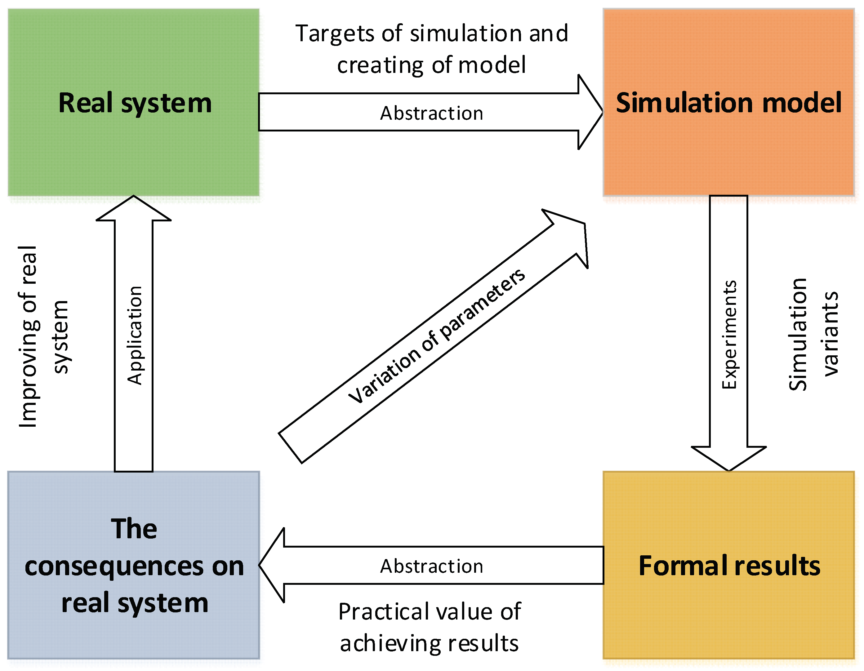
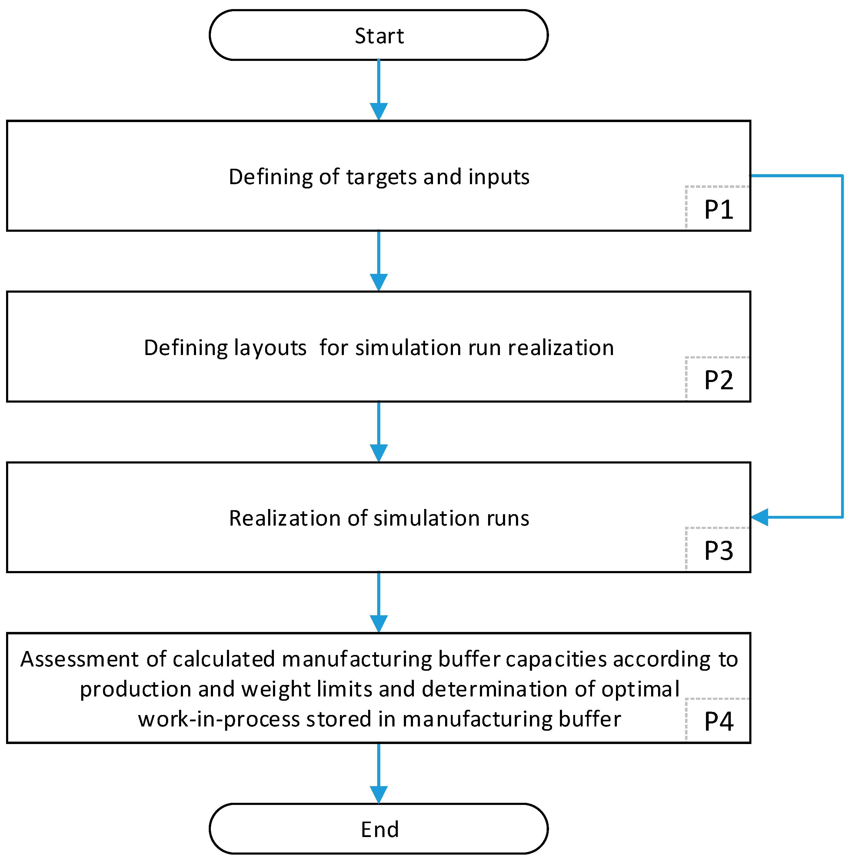
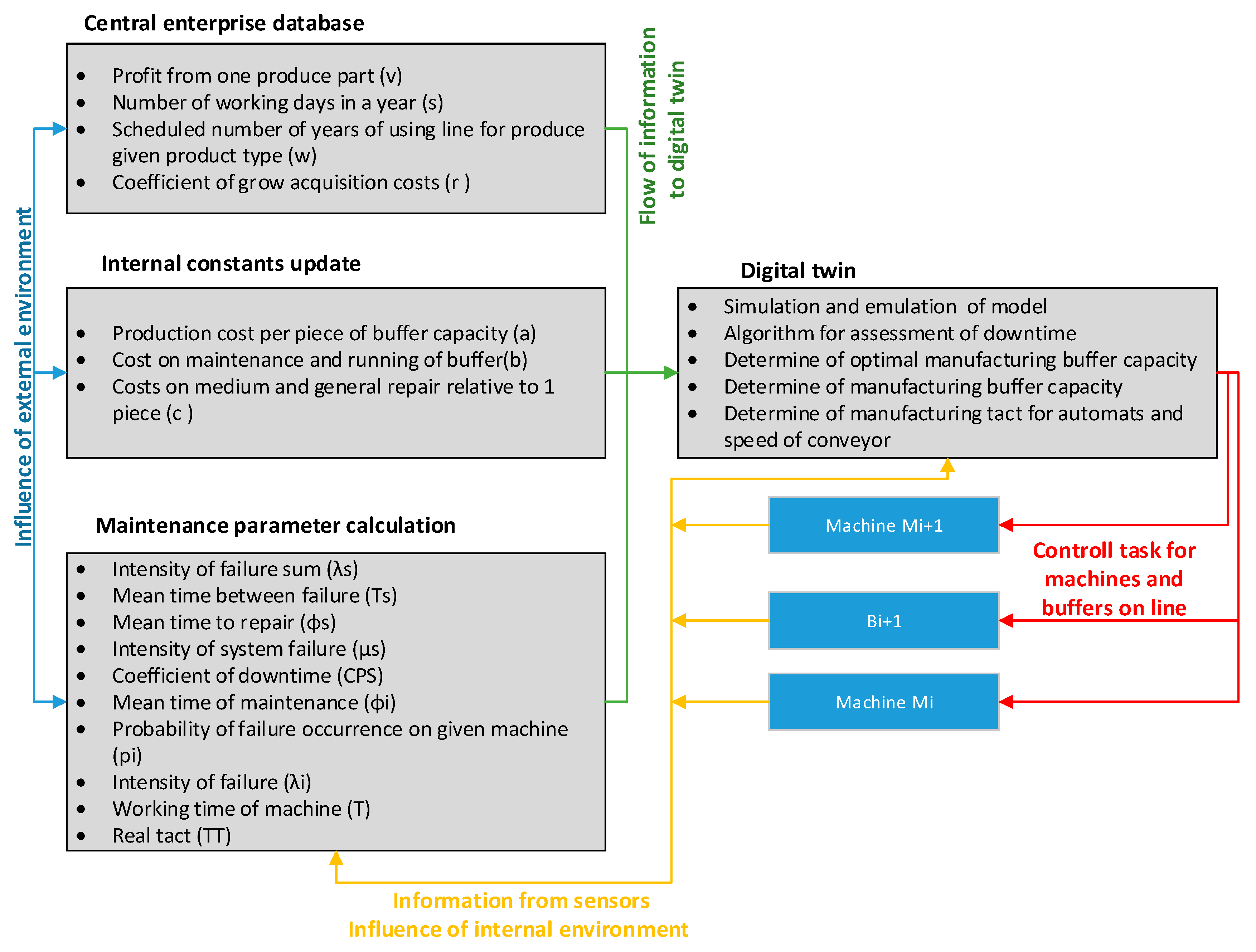
The current situation in the field of interoperation manufacturing buffer is a combination of using conveyers for the functions of manufacturing buffers and common manufacturing buffers. To make manufacturing competitive and sustainable, it is necessary to actively seek to avoid waste in production. Waste in production also includes a high level of buffer inventory. The cost of inventory is mainly manifested by the use of capital that could have been used for another purpose. WIP inventory is, therefore, a cost item, and is required to be as low as possible. To reduce the WIP inventory, it is necessary for the optimum capacity of the manufacturing buffer to be calculated for each group of products before each device is added to the manufacturing line. For the process of determining the optimal capacity of manufacturing buffers, the system described below was created. Mutual interactions and relationships are defined for each block of the algorithm. The phases of this system are shown in Figure 4. The system is suitable for already operating production systems, and statistics from devices can be obtained.

3.1.1. Definitions of Targets and Inputs

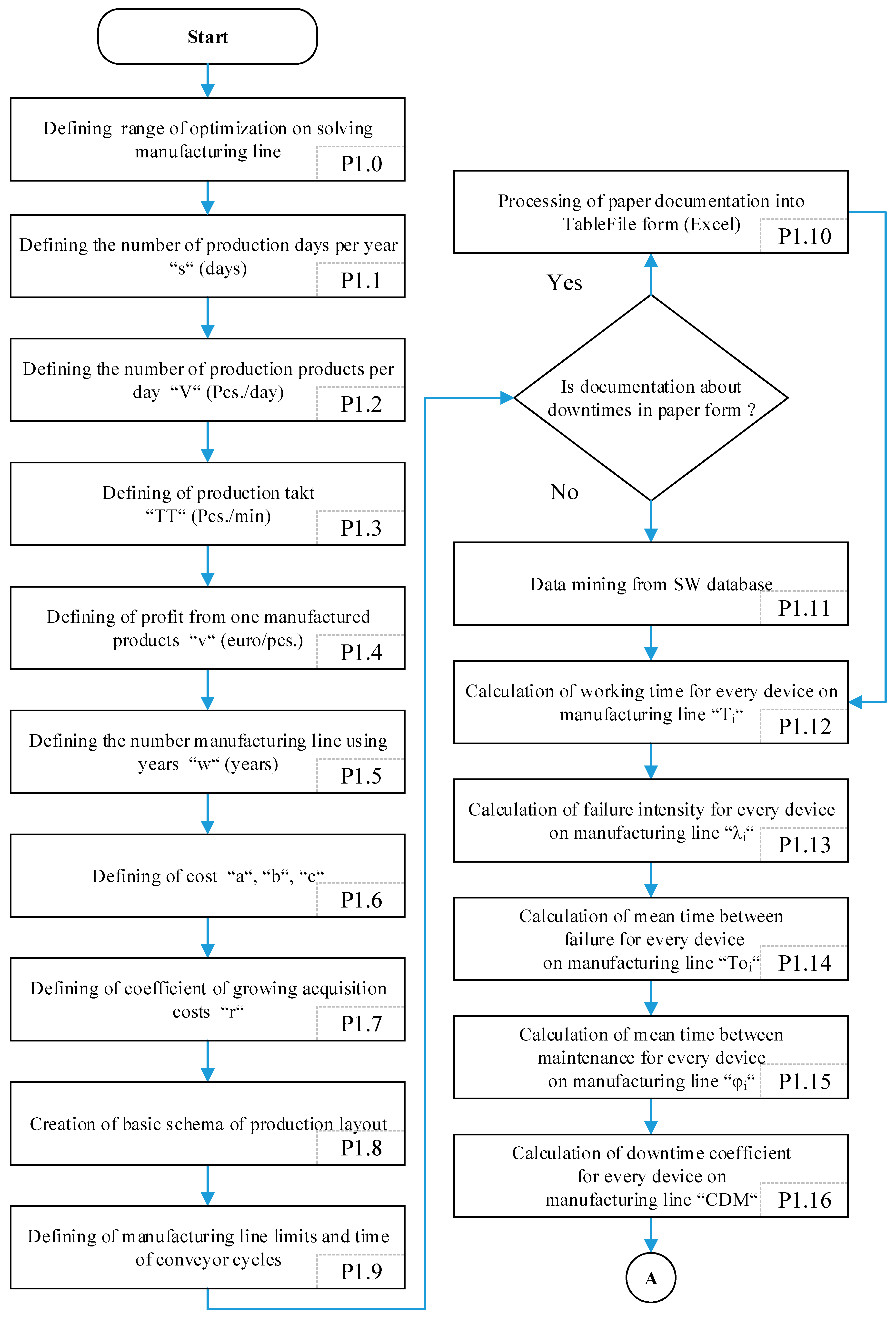
The main goal of the first phase of the definition of targets and inputs is to determine the extent of the solvable manufacturing line parts and the objectives of optimisation. This phase also includes the collection and processing of all necessary data needed to determine the optimum capacity of the manufacturing buffer and, thus, the optimal WIP inventory. The data obtained in the later phase serve as input for the realisation of calculations. The contents of the algorithm for defining targets and inputs are illustrated in Figure 5. The definition of targets can be understood as the selection of a manufacturing line range with defined limitations causing negative impacts that are exceeded by the benefits. Inputs are understood as data related to devices on the manufacturing line that ensure the validity of the simulation model to represent the real situation.

Block P1.0, at the beginning of the optimisation process, is necessary to define the objectives according to which WIP inventory optimisation of the range of the production line will be carried out.

Block P1.1 represents the determination of the number of production days per year. The parameter includes only the production days when the product for which the calculation of the optimal WIP inventory is intended is being produced. This can be estimated from the number of planned manufactured products pulled from a marketing survey and orders [21].

Block P1.2 represents the determination of the production volume for the entire shift (V). It is given in pieces for all shifts per day (the best results can be achieved by considering two shifts [11]). This is the maximum throughput that the manufacturing line is able to achieve without downtime. It can be determined based on the cycle time of automatic machines.

Block P1.3 represents the identification of the cycle time of the automatic machine (ϑ). It is given in pieces per minute and converted into pieces per hour. It should be the cycle time of an automatic machine that is a bottleneck in the system.

Block P1.4 represents the determination of the profit that comes from one product (v). It is given in monetary units per piece. It is calculated as the unit cost of production subtracted from the selling price.

Block P1.5 represents the number of years (w) for which the production of the product is planned. It is a dynamic indicator and depends mainly on the market and its requirements. The planned production time can be determined based on marketing forecasts and orders.

Block P1.6 represents the determination of the unit cost of production of the manufacturing buffer capacity with the following characteristics:

(a) It is given in monetary units per piece. They are understood as storage costs. Storage costs create an effect where capital is tied to materials and cannot be used elsewhere. The capital-binding materials generate costs calculated from their price with the aid of any of the evaluation methods.

(b) It represents the running and maintenance costs of the manufacturing buffer. It is given in monetary units per manufacturing buffer for all shifts (the best results can be achieved by considering two shifts [11]). Its value can be calculated from the cost of lubricating the manufacturing buffer mechanisms. In the case of sensors, it is the cost of energy, the work done to control the sensors and, where appropriate, the cleaned contents of the manufacturing buffer after a variety of hardened emulsions mixed with impurities. They are activities that are carried out every day. The determination of maintenance costs consists of taking the findings of each day for repetitive acts, measuring their time costs and multiplying the duration by the hourly added value of the manufacturing line.

(c) It represents the determination of the costs of medium and general repair of the manufacturing buffer. It is given in monetary units for one manufacturing buffer. This is the cost of planned manufacturing buffer repairs that do not occur every day; they are planned ahead using predictive maintenance. They may be repaired outside the total productive maintenance (TPM) [20] of machines, which suspends the manufacturing line and creates costs. The cost depends on different factors like the needs of the professional and the cost of performing the repairs, e.g., the need for the replacement of mechanisms or sensors, the duration of the repair, etc. All such factors need to be considered, and they approximately determine the duration of the intervention and the costs of medium and general repair. The costs of medium and general repair can be found by multiplying the duration of the activity by the hourly added value of the manufacturing line.

Block P1.7 represents the determination of the factor that determines the growth of the acquisition and repair costs (r). Its value should be 1 ≤ r. Based on [11], the ideal value of this coefficient is 1.5.

Block P1.8 represents the acquisition or outline of a layout with the deployment and naming of devices (automatic machines) on the manufacturing line.

Block P1.9 represents the detection of all restrictions that occur on the line. At the same time, the cycles of individual conveyors must be measured.

The decision block represents the assessment in the form of documentation. If it is in paper form, it is necessary to insert all data about the failure into Excel for further work. If the failure data are inserted into any database software, it is necessary to pull all downtime data from the database.

Block P1.12 is the calculation of the devices’ running time (T_i) [20]. It is given in hours:

$$T_i= \mathsf{\Sigma }\mathrm{P}{T}_i-\mathsf{\Sigma }{\mathsf{\eta }}_{\mathrm{i}},$$

(6)

where PT_i is the planned the working time of the i-th device and η_i is the overall length of downtime of the i-th device during the planned working time.

Block P1.13 represents the calculation of the failure intensity (λ_i) on all devices on the manufacturing line [20]:

$${\mathsf{\lambda }}_{\mathrm{i}}=\frac{{COD}_i}{T_i},$$

(7)

where COD_i is the overall downtime that occurs during the running time of the i-th device.

Block P1.14 represents the calculation of the mean time between failures (MTTR) for the i-th device (To_i) counted for every device on the manufacturing line [20]. It is given in hours:

$$T{o}_i= \frac{T_i}{CO{D}_i} .$$

(8)

Block P1.15 represents the calculation of the mean maintenance time for the i-th device (Φ_i) counted for every device on the manufacturing line [20]. It is given in hours:

$${\mathsf{\Phi }}_i= \Sigma ({\mathsf{\eta }}_i\ast CO{D}_i).$$

(9)

Block P1.16 represents the calculation of the coefficient of downtime (CDM) for every device located on the manufacturing line [20]. It is given as a percentage:

$$\mathrm{CDM}= \frac{{\mathsf{\Phi }}_{\mathrm{i}}}{{\mathsf{\Phi }}_{\mathrm{i}}+{\mathrm{To}}_{\mathrm{i}}}.$$

(10)

The value of availability is calculated for each device using (CDM) [20]:

$$\mathrm{availability}=100-\mathrm{CDM}.$$

(11)

If the manufacturing line is transferred, it can be used to calculate the coefficient of downtime of the manufacturing line (CDS), which is used for the calculation (CDM).

3.1.2. Defining Layouts for Simulation Run Realisation

The manufacturing line decomposition module is used to create the schemas needed to create a simulation model in accordance with the submodule of the optimal manufacturing buffer capacity calculation and the objective function value. The input data include block P1.8. The result of this phase is the creation of the layout of a solvable manufacturing line according to which the simulation models are carried out. A diagram of the defining layouts for simulation run realisation is shown in Figure 6.

The purpose of block P2.1 is to determine the number of solvable layout parts of the manufacturing line based on the decomposition strategy. To calculate the number of layout parts in the manufacturing line, the number of machines must be divided by three. The number three is used as it is the number of automatic machines with two manufacturing buffers. The optimal capacity is calculated using three automatic machines and two manufacturing buffers because that is the simplest example of the interactions between manufacturing buffers. With two manufacturing buffers, the impact of their capacity on the objective function can be observed. At the same time, the understanding of the line of three automatic machines and two manufacturing buffers helps us to deal with longer and much more complex manufacturing lines [11]. A graphical expression of the decomposition process for three machines and two manufacturing buffers is shown in Figure 7.

The principle of decomposition lies in the gradual solution of the manufacturing line, starting from the first automatic machine, and each calculated solution becomes a constant for the next solved part.

In the case of a branch, the part must be solved as a problem of two automatic machines and one manufacturing buffer [11]. A graphical expression of the decomposition process for two machines and one manufacturing buffer is shown in Figure 8.

Each part (A or B) creates a separate part of the manufacturing line for the realisation of simulation runs, and the objective function is calculated separately for B1 and B2.

This decomposition of the line is possible because the throughput of part of the system is given by the last machine parameter [22].

3.1.3. Realisation of Simulation Runs

The module serves as an algorithm to obtain the results of the downtime η at different manufacturing buffer capacities. The input data come from blocks P1.9, P1.15 and P1.16. In these blocks, there are data about the parameters of the machines and conveyors. Other input data include simulation schematics obtained from block P2.1. A schema of the phase realisation of simulation runs is shown in Figure 9.

Block P3.1 represents the creation of a simulation model for the first part of the manufacturing line based on the data from the input module and the layout obtained from the decomposition module.

Block P3.2 represents the realisation of simulation experiments with the created model. First, it is run with the maximum capacity of the manufacturing buffer obtained based on the volume or weight calculation.

The volume calculation (CB_i) [20] is

$$C{B}_i= \frac{WC{B}_i}{VS},$$

(12)

where WCB_i is the total volume of the manufacturing buffer after the subduction of mechanical restraints, and VS is the volume of one product placed in the manufacturing buffer calculated according to the widest size of the product.

The weight calculation (CB_i) [20] is

$$C{B}_j= \frac{MW{B}_i}{WS},$$

(13)

where MWB_i is the maximum weight load of the manufacturing buffer, and WS is the weight of the single product. Note that the number with the smallest value is selected.

The data about the average state of the manufacturing buffer and the CDS of the manufacturing lines are the starting points for comparing the results obtained in block P3.4.

Block P3.3 represents the number of experiments that will be carried out to obtain the maximum objective function, which is represented by the optimum and can be found as an extreme of the objective function. The objective function is chosen as the optimisation criterion. Based on the selected calculation according to Maixner [11], if the current average capacity of the manufacturing buffer does not interfere with the current MTTR or the availability of a maximum limit by weight or volume, it represents the upper limit. In case of a solution to the problem of three machines and two manufacturing buffers, and if it is an upper limitation, a high value rounded up to a multiple of 10 is a good upper limit. Then, the number is divided by 10, and the incrementation step is complete. Consequently, after the analysis of the results, the highest objective function is chosen, and it goes on searching near the area with incrementation of one piece. To solve the problem of two machines and one manufacturing buffer, there is no limitation on carrying out the experiments, as it is a one-way matrix without multiplying combinatorist options.

Block P3.4 aims to realise the simulation run, which gradually changes the capacity of the manufacturing buffer, thereby obtaining the downtime.

Block P3.5 represents the enrolment of data from the simulation results to the matrix of the downtime η. These data are used for the calculation of the objective function.

The purpose of block P3.6 is to create an algorithm that calculates the value of objective function (G). After determination (Gmax), it is possible to determine the optimum capacity of the manufacturing buffer. A block schema, called a block of optimal manufacturing buffer capacity, and the objective function calculation are shown in Figure 10.

The decision block is used to decide whether the result is comparable to the coefficient of the line downtime, which has a fixed bond, or to a manufacturing line with a specific coefficient of downtime. The coefficient of downtime can be found by simulation or by processing a document related to downtime on the manufacturing line.

Blocks P3.5.2 to P3.5.7 are used to calculate the coefficient of line downtime with a fixed bond.

After the determination of the coefficient of downtime, the calculation of objective function (G) can start. Blocks P3.5.8 to P3.5.11 are used to calculate the parameters that are put in the final formula (G) in block P3.5.12. The value (G) is different for each manufacturing buffer capacity. For calculation (G), all input data must be defined or calculated. The objective function (G) is the total benefit of the application of the selected manufacturing buffer capacity over the entire period. Thanks to (G), it is possible to determine the optimum manufacturing buffer capacity [11].

In block P3.5.13, after determining all the values (G) at different manufacturing buffer capacities, (Gmax) can be found. (Gmax) is the maximum objective function value. After the selection of (Gmax), the capacity of the manufacturing buffer that corresponds to (Gmax) is determined.

Block P 3.7 involves the determination of the optimal manufacturing buffer capacity for the solving part of the manufacturing line.

The decision-making block chooses whether to continue with simulating the next part of the manufacturing line or whether all parts of the manufacturing line are resolved and can be processed to assess the calculated manufacturing buffer capacity according to the production and weight limits and the determination of the optimal WIP inventory stored in the manufacturing buffer.

If all parts of the manufacturing line are not solved, block P3.8 creates a new simulation model. The new simulation model is created based on input data parameters and the schematic of the next part of the manufacturing line.

3.1.4. Assessment of Calculated Manufacturing Buffer Capacities According to Production and Weight Limits and Determination of the Optimal Work-in-Progress Stored in the Manufacturing Buffer

The module is used to evaluate the calculated optimum manufacturing buffer capacity according to the production restrictions of the automatic machines. A schema of the assessment of calculated manufacturing buffer capacities according to production and weight limits and determination of the optimal work-in-progress stored in the manufacturing buffer algorithm stages is shown in Figure 11.

The entry decision block determines whether the average annual state of the manufacturing buffer is obtained by simulating P4.2 or by observing manufacturing line P4.1.

Block P4.3 represents the determination of the average manufacturing buffer capacity ((Bp_i), (Bp_j). It represents the quantity at which, in production without restrictions, production machines can produce the manufacturing buffer.

The decision blocks behind block P4.3 represent a comparison (Bp_i) and (Bp_j) with the calculated optimum capacity (Bopt_i) and (Bopt_j). Based on the comparison, (Bopt_i) or (Bp_i) is selected. At first, in the blocks, the manufacturing buffer capacity is assessed, and the production limit result is determined as the quantity that is to be maintained in the manufacturing buffer. The sum of the capacity to be maintained in manufacturing buffers represents the optimal WIP inventory for that part of the production line.

3.2. Case Study

3.2.1. Defining the Targets and Inputs

Verification and validation of the proposed algorithm were carried out on a production line in a manufacturing company in the automotive industry. The manufacturing process consists of grinding (MOL3VER, GR1065), honing (KM85A1, KM85A2, KM85B1, KM85B2), washing with a nozzle (ST1 washing, ST2 turn, ST3 washing, ST1B washing, ST2B turn, ST3B washing) and a series of assembly operations (weight measure 1, dimension measure 1, weight measure 2, dimension measure 2, 13 stations and visual check) connected with conveyors, as shown in Figure 9. The main criterion for assessment was whether the solution achieved was better than the current state. In other words, the benefit from the introduction of the optimal manufacturing buffer capacities should be greater than the benefit of maintaining the current state. Another criterion is that the loss of throughput should not be more than 2%. To solve and optimise the WIP inventory, grinding line A was selected. The layout used to solve this production line is illustrated in Figure 12. The red, dashed, bounded line represents the grinding line A. The yellow line is grinding line B, and the last assembly zone has no boundary.

The conveyors are used on the chosen production line as the manufacturing buffer. To determine the optimal WIP of grinding line A, it was necessary to determine the optimum capacity of manufacturing buffers B2, B3, B4, B5 and B6. For the creation of the manufacturing line simulation model, the MTTR, availability and cycle time parameters were identified, as summarised in

Table 1. Simulation input information about the devices on the manufacturing line.

Shortcut of Device	MTTR (min)	Availability (%)	Cycle Time (min)
MOL3VER	7:00	99	0:06.5
KM85A1	6:00	99	0:10.8
KM85A2	7:00	99	0:11.3
ST1 washing	0 1	100 1	0:05.3
ST2 turn	0 1	100 1	0:03.5
ST3 washing	1:00	99	0:05
Weight measure 1	1:00	99	0:06.3
Dimension measure 1	1:00	99	0:05
GR1065	9:00	99	0:06.7
KM85B1	7:00	99	0:10.3
KM85B2	7:00	99	0:10.9
ST1B washing	1:00	99	0:03.1
ST2B turn	0 1	100 1	0:06.9
ST3B washing	1:00	98	0:05
Weight measure 2	1:00	99	0:06.3
Dimension measure 2	1:00	99	0:05
ST1	10:00	89	0:06.3
ST2	10:00	91	0:06.3
ST3	1:00	99	0:06.3
ST4	10:00	91	0:06.3
ST5	1:00	99	0:06.3
ST6	10:00	91	0:06.3
ST7	1:00	99	0:06.3
ST8	1:00	99	0:06.3
ST9	1:00	97	0:06.3
ST10	1:00	99	0:06.3
ST11	1:00	99	0:06.3
ST12	5:00	95	0:06.3
ST13	1:00	97	0:06.3
Visual check	0 1	100 1	0:05.5

¹ No historical record of downtime.

. The data were analysed for three months.

The parameters for conveyors functioning as manufacturing buffers placed on the solving line are shown in

Table 2. Simulation input information about the conveyors on the manufacturing line.

Shortcut of Conveyor	Max Capacity (Pcs.)	Cycle Time (min)	Length (m)
B1	22	0:04.29	4.29
B2	39	0:08.36	8.36
B3	9	0:01.7	1.72
B4	53	0:10.49	10.49
B5	6	0:01.48	1.48
B6	11	0:02	2.00
B7	8	0:01.52	1.50
B8	35	0:06.96	6.96
B9	5	0:01	1.00
B10	39	0:07.69	7.69
B11	6	0:01	1.00
B12	49	0:09.64	10.64
B13	4	0:00.6	0.6
B14	4	0:00.6	0.6
B15	3	0:00.5	0.5
B16	7	0:01.29	1.29
B17	5	0:01	0.89
B18	3	0:00.5	0.5
B19	3	0:00.5	0.5
B20	10	0:01	1

. An availability of 100% and an MTTR value of manufacturing buffers of 0 were considered.

The supply of production processes on inputs has no downtime. The value (CDS) for the solving line is determined by the simulation from the last device in the line; in our case, for grinding line 1, it is dimension measure 1, CDS = 52.61%.

The input data required for the calculation of the objective function are summarised in

Table 3. Input parameters for calculation of the objective function.

Parameter	Value
s	20
V	13,291
ϑ	9.23
v	0.52
w	2
a	10
b	0.5
c	5
r	1.5

.

The values of the cost constants of the manufacturing buffer (a, b, c) that are noted above were modelled using the characteristics of production. Each production has different values, and they are influenced by their processes [11].

3.2.2. Defining Layouts for Simulation Run Realisation

For validation and verification, the selected production line was divided into parts, as shown in Figure 13.

The optimisation of the line was divided into four solvable parts. Layouts Rl1, Rl2 and Rl4 can be used to solve two machines and one manufacturing buffer. Layout Rl3 can be used to solve three machines and two manufacturing buffers. Layout Rl1 in Figure 13 (red area) contains machines MOL3VER and KM85A2, and the manufacturing buffer is B2. Layout Rl2 in Figure 13 (yellow area) contains machines MOL3VER and KM85A1, and the manufacturing buffer is B3. Layout Rl3 in Figure 13 (purple area) contains machines KM85A1 and KM85A2, the series of station ST washing, ST2 turn, and ST3 washing, and manufacturing buffers B4 and B5. Layout Rl4 in Figure 13 (blue area) contains the series of station ST washing, ST2 turn, and ST3 washing and the series of station weight measure 1 and dimension measure 1. The manufacturing buffer is B6.

3.2.3. Realisation of Simulation Runs

By carrying out a simulation on a simulation model in which the capacity of the manufacturing buffer was limited to the maximum capacity found through the volume or weight calculation, the following average inventory of the manufacturing buffers was found. These average manufacturing buffer states are listed in

Table 4. Average manufacturing buffer inventories.

Shortcuts of Manufacturing Buffers	The Average Manufacturing Buffer Content
B2	4
B3	4
B4	53
B5	8
B6	11

.

By finding the inventory state of the manufacturing buffers, the buffers’ capacities could be used, at the same time, to represent the production restriction value of the manufacturing line (Bp). The values (CDS) for the solvable manufacturing line parts are given in

Table 5. CDS and CDC values for the solvable parts of the manufacturing line.

Layout Shortcuts of the Manufacturing Line	CDS (%)	CDC (%)
Rl1	47.10	60
Rl2	48.15	60
Rl3	52.60	60
Rl4	52.61	60

. The task is to ensure that there is no increase in CDS against the original value outside the tolerance threshold of a 2% decrease in the throughput, which is defined in the optimisation objectives. At the same time, the condition that the proposed solution exceeds the benefits of the current solution must be fulfilled.

For calculation purposes, because it is not compared with a fixed bounding line, the CDC values in Table 5 were chosen.

The experimental results of downtime η for solving layout Rl1 show

Table 6. Matrix of downtime η for the tested capacity of the manufacturing buffer for layout Rl1.

Capacity	η (%)	Capacity	η (%)	Capacity	η (%)	Capacity	η (%)
1	47.563207	11	47.090758	21	47.071140	31	47.069832
2	47.206159	12	47.083564	22	47.070486	32	47.069832
3	47.150920	13	47.080295	23	47.069832	33	47.069832
4	47.137496	14	47.077025	24	47.069832	34	47.069832
5	47.131956	15	47.075717	25	47.069832	35	47.069832
6	47.122800	16	47.073755	26	47.069832	36	47.069832
7	47.115608	17	47.073101	27	47.069832	37	47.069832
8	47.107760	18	47.072447	28	47.069832	38	47.069832
9	47.103836	19	47.071793	29	47.069832	39	47.069832
10	47.095335	20	47.071140	30	47.069832	40	47.069832

and Figure 14. Based on the input data and downtime data, the objective function G was calculated to solve layout Rl1, as shown in

Table 7. Matrix of objective function G for the tested capacity of the manufacturing buffer for layout Rl1.

Capacity	G (euros)	Capacity	G (euros)	Capacity	G (euros)	Capacity	G (euros)
1	34,347.38	11	34,921.25	21	33,879.22	31	32,537.34
2	35,287.04	12	34,844.85	22	33,756.70	32	32,391.06
3	35,384.23	13	34,754.34	23	33,631.79	33	32,242.79
4	35,359.29	14	34,660.71	24	33,502.72	34	32,092.56
5	35,306.90	15	34,558.66	25	33,371.35	35	31,940.41
6	35,259.46	16	34,455.50	26	33,237.73	36	31,786.35
7	35,202.00	17	34,345.92	27	33,101.91	37	31,630.42
8	35,142.08	18	34,233.60	28	32,963.92	38	31,472.63
9	35,067.34	19	34,118.64	29	32,823.80	39	31,313.03
10	35,001.50	20	34,001.09	30	32,681.60	40	31,151.62

and Figure 15.

The behaviour of the curve in Figure 14 shows that the manufacturing buffer capacity downtime decreases until point 12, after which no decrease occurs. The curve in Figure 15 shows that, as the manufacturing buffer capacity increases, the assets increase until point 3, which is marked as the local extreme; after this point, a decrease occurs. Table 7 and Figure 15 show the local optimum, which appears as an extreme towards the plus values. In our case, this value is 35,384.24, which corresponds to a value of three pieces in manufacturing buffer B2. The value of three pieces in manufacturing buffer B2 stays constant in the next calculations.

The experimental results of the downtime η for solving layout Rl2 and the objective function calculated based on the downtime and input information are shown in

Table 8. Matrix of the downtime η and objective function G for the tested capacity of the manufacturing buffer for layout Rl2.

Capacity	η (%)	G (euros)
1	48.217759	32,537.82
2	48.194022	32,556.02
3	48.179022	32,541.97
4	48.179022	32,479.92
5	48.178999	32,412.27
6	48.171249	32,360.95
7	48.173396	32,277.66
8	48.172146	32,199.51
9	48.168125	32,125.04
10	48.168124	32,035.70

. A graphical expression of the downtime η and objective function G for solving layout Rl2 is shown in Figure 16.

The behaviour of the curve in Figure 16a shows that with an increase in the manufacturing buffer capacity, the downtime decreases most steeply until point 3; after that point, the decrease is not so steep. The curve in Figure 16b shows that, as the manufacturing buffer capacity increases, the assets increase until point 2, which is marked as the local extreme; after this point, a decrease occurs. From Table 8 and Figure 16b, the local optimum can be found, which appears as an extreme towards the positive values. In our case, this value is 32,556.02, which corresponds to a value of two pieces in manufacturing buffer B3. This value of two pieces in manufacturing buffer B3 stay as a constant in the next calculations.

In the case of solution layout Rl3, it can be seen that it is necessary to validate the capacity of 60 in manufacturing buffer B4 and the capacity of 10 in manufacturing buffer B5; together, this involves 600 experiments. To reduce the computational difficulty, experiments were carried out in two phases. In the first phase, the capacity of manufacturing buffer B4 increased in increments of five and manufacturing buffer B5 increased in increments of one, so 120 experiments were required. In the next phase, after the calculation of the objective function, the range ±5 capacity from the identified optimal objective function was selected for testing, so 100 experiments were required. The experimental results of downtime η for solving layout Rl3 phase 1 are shown in

Table 9. Matrix of the downtime η for the tested capacity of the manufacturing buffer for layout Rl3 phase 1.

η (%)		B4 Capacity
		5	10	15	20	25	30	35	40	45	50	55	60
B5 Capacity	1	51.661399	51.622337	51.587614	51.552892	51.510936	51.470427	51.442938	51.425577	51.418343	51.411110	51.409663	51.409663
	2	51.648378	51.613656	51.578934	51.544212	51.502256	51.464640	51.438598	51.424131	51.416897	51.409663	51.409663	51.409663
	3	51.641144	51.609316	51.574593	51.535531	51.493575	51.458853	51.434258	51.422684	51.415450	51.409663	51.409663	51.409663
	4	51.636804	51.602082	51.567360	51.526850	51.486341	51.451619	51.431364	51.421237	51.414003	51.409663	51.409663	51.409663
	5	51.633911	51.597742	51.563019	51.519617	51.477661	51.445832	51.428471	51.419790	51.412556	51.409663	51.409663	51.409663
	6	51.628124	51.591955	51.555786	51.512383	51.468980	51.441492	51.425577	51.418343	51.411110	51.409663	51.409663	51.409663
	7	51.625230	51.589061	51.551445	51.505149	51.463193	51.437151	51.424131	51.416897	51.409663	51.409663	51.409663	51.409663
	8	51.622337	51.584721	51.544212	51.499362	51.457406	51.434258	51.422684	51.415450	51.409663	51.409663	51.409663	51.409663
	9	51.622337	51.584721	51.544212	51.499362	51.457406	51.434258	51.422684	51.415450	51.409663	51.409663	51.409663	51.409663
	10	51.622337	51.584721	51.544212	51.499362	51.457406	51.434258	51.422684	51.415450	51.409663	51.409663	51.409663	51.409663

and Figure 17a. The objective function is illustrated in

Table 10. Matrix of objective function G for the tested capacity of the manufacturing buffer for layout Rl3 phase 1.

G		B4 Capacity
		5	10	15	20	25	30	35	40	45	50	55	60
B5 Capacity	1	22,749.93	22,451.29	22,050.20	21,575.97	21,058.60	20,480.84	19,815.64	19,074.85	18,261.54	17,406.28	16,495.21	15,542.21
	2	22,738.50	22,427.86	22,026.77	21,552.54	21,035.17	20,449.41	19,780.22	19,031.42	18,218.12	17,362.85	16,447.79	15,494.78
	3	22,702.98	22,384.34	21,983.25	21,521.02	21,003.66	20,409.90	19,736.70	18,979.91	18,166.60	17,307.34	16,392.27	15,439.27
	4	22,652.93	22,342.28	21,941.19	21,482.96	20,961.60	20,367.84	19,682.64	18,921.85	18,108.54	17,245.28	16,330.21	15,377.21
	5	22,593.22	22,286.57	21,885.49	21,435.26	20,917.89	20,316.13	19,622.94	18,858.14	18,044.84	17,177.57	16,262.51	15,309.50
	6	22,536.47	22,229.82	21,832.74	21,382.51	20,869.14	20,255.38	19,558.19	18,789.39	17,976.09	17,104.82	16,189.76	15,236.75
	7	22,467.12	22,160.47	21,767.39	21,325.16	20,807.79	20,190.03	19,484.84	18,716.04	17,902.74	17,027.47	16,112.41	15,159.40
	8	22,393.51	22,090.87	21,705.78	21,259.55	20,742.18	20,116.42	19,407.23	18,638.44	17,821.13	16,945.87	16,030.80	15,077.80
	9	22,307.92	22,005.28	21,620.19	21,173.96	20,656.59	20,030.83	19,321.64	18,552.85	17,735.54	16,860.28	15,945.21	14,992.21
	10	22,218.58	21,915.94	21,530.85	21,084.62	20,567.25	19,941.49	19,232.30	18,463.50	17,646.20	16,770.94	15,855.87	14,902.87

and Figure 17b.

The shape of the graph in Figure 17a shows that, as the manufacturing buffer capacity increases, the downtime decreases most steeply until point 30; after that, the decrease is not so steep. The surface of the graph in Figure 17b shows that the most benefit to the assets occurs at around point 5 for B4 and in the range of 1‒10 for B5. Otherwise, the surface of the objective function decreases over the whole range of B4. Table 10 and Figure 17b show that the local optimum appears as an extreme towards the positive values. In our case, this value is 22,749.94, which corresponds to a value of five pieces in manufacturing buffer B4 and one piece in manufacturing buffer B5. Based on these numbers, B4(5) and B5(1), the optimum values in phase 2 are a B4 manufacturing buffer capacity ranging from one to 10 pieces and a B5 manufacturing buffer ranging from one to 10 pieces. The experimental results of the downtime η for solving layout Rl3 phase 2 are shown in

Table 11. Matrix of the downtime η for the tested capacity of the manufacturing buffer for layout Rl3 phase 2.

η [%]		B4 Capacity
		1	2	3	4	5	6	7	8	9	10
B5 capacity	1	53.144363	53.125073	53.112052	53.101443	53.089869	53.079741	53.070096	53.061898	53.055146	53.048395
	2	53.136165	53.113017	53.101925	53.090351	53.079741	53.069132	53.061416	53.054182	53.047913	53.041161
	3	53.135200	53.102889	53.091315	53.081670	53.070096	53.061416	53.055146	53.047913	53.042126	53.034892
	4	53.135200	53.094209	53.084564	53.072507	53.063345	53.055146	53.049359	53.041643	53.035374	53.028140
	5	53.135200	53.087457	53.075883	53.065274	53.057558	53.050324	53.043572	53.036821	53.030069	53.023318
	6	53.135200	53.081188	53.070096	53.061898	53.053700	53.045501	53.038267	53.031998	53.025247	53.017048
	7	53.135200	53.076365	53.067203	53.059004	53.049842	53.041161	53.033927	53.027176	53.019942	53.013190
	8	53.135200	53.073472	53.063827	53.054664	53.045501	53.036821	53.029105	53.022835	53.015119	53.008368
	9	53.135200	53.073472	53.063827	53.054664	53.045501	53.036821	53.029105	53.022835	53.015119	53.008368
	10	53.135200	53.073472	53.063827	53.054664	53.045501	53.036821	53.029105	53.022835	53.015119	53.008368

and Figure 18a. The objective function is illustrated in

Table 12. Matrix of objective function G for the tested capacity of the manufacturing buffer for layout Rl3 phase 2.

G		B4 Capacity
		1	2	3	4	5	6	7	8	9	10
B5 Capacity	1	18,882.88	18,888.78	18,869.26	18,836.54	18,800.83	18,756.08	18,705.39	18,646.45	18,579.52	18,508.85
	2	18,858.12	18,874.69	18,849.83	18,819.77	18,781.40	18,737.98	18,681.96	18,620.35	18,552.10	18,481.42
	3	18,805.27	18,847.17	18,823.65	18,788.26	18,752.55	18,703.80	18,643.78	18,582.17	18,512.58	18,443.24
	4	18,743.21	18,809.11	18,780.26	18,751.53	18,709.16	18,659.07	18,597.72	18,537.44	18,469.19	18,399.84
	5	18,675.50	18,760.07	18,736.55	18,703.82	18,657.45	18,604.70	18,546.01	18,483.07	18,416.15	18,345.47
	6	18,602.76	18,704.65	18,679.80	18,640.41	18,595.37	18,545.28	18,487.93	18,423.65	18,356.73	18,290.05
	7	18,525.41	18,640.63	18,610.45	18,571.06	18,528.68	18,479.93	18,422.58	18,359.64	18,294.05	18,223.37
	8	18,443.80	18,567.02	18,538.17	18,501.45	18,459.07	18,410.32	18,354.30	18,290.03	18,225.77	18,155.09
	9	18,358.21	18,481.44	18,452.58	18,415.86	18,373.48	18,324.73	18,268.71	18,204.44	18,140.18	18,069.51
	10	18,268.87	18,392.09	18,363.24	18,326.52	18,284.14	18,235.39	18,179.37	18,115.10	18,050.84	17,980.16

and Figure 18b.

The shape of the graph in Figure 18a shows that, with an increase in the manufacturing buffer capacity, the downtime decreases. The surface of the graph in Figure 18b shows that the most benefit occurs inside the area bounded by B5(3) and B4(4). From Table 12 and Figure 18b, the local optimum can be found, which appears as an extreme towards the positive values. In our case, this value is 18,888.79, which corresponds to a value of two pieces in manufacturing buffer B4 and one piece in manufacturing buffer B4. Layout Rl3, therefore, gives the optimum manufacturing buffer capacity for B4 (2) and B5 (1).

The experimental results of the downtime η for solving layout Rl4 are shown in

Table 13. Matrix of downtime η and objective function G for the tested capacity of the manufacturing buffer for layout Rl4.

Capacity	η (%)	Capacity	η (%)	Capacity	G (euros)	Capacity	G (euros)
1	53.750041	11	53.414393	1	17,243.44	11	17,439.12
2	53.703744	12	53.414393	2	17,324.00	12	17,342.83
3	53.658091	13	53.414393	3	17,394.70	13	17,243.28
4	53.616296	14	53.414393	4	17,448.19	14	17,140.62
5	53.577073	15	53.414393	5	17,488.92	15	17,034.94
6	53.542350	16	53.414393	6	17,512.16	16	16,926.36
7	53.510200	17	53.414393	7	17,523.69	17	16,814.97
8	53.481265	18	53.414393	8	17,522.08	18	16,700.85
9	53.454902	19	53.414393	9	17,509.37	19	16,584.08
10	53.433040	20	53.414393	10	17,480.47	20	16,464.72

and the graphical expression is shown in Figure 19a. The objective function is calculated in Table 13, and its graphical expression is shown in Figure 19b.

The behaviour of the curve in Figure 19a shows that as the manufacturing buffer capacity increases, the downtime decreases until point 11; after that point, no decrease occurs. The curve in Figure 15 shows that, as the manufacturing buffer capacity increases, the assets increase until point 7, which is marked as the local extreme; after this point, a decrease occurs. From Table 13 and Figure 19b, the local optimum can be found, which appears as an extreme towards the positive values. In our case, this value is 17,523.70, which corresponds to a value of seven pieces in manufacturing buffer B6.

3.2.4. Assessment of Calculated Manufacturing Buffer Capacities According to the Production and Weight Limits and Determination of the Optimal Work-in-Progress Stored in the Manufacturing Buffer

A comparison of the calculated optimum manufacturing buffer capacity (B_opt) and the manufacturing buffer capacity production limitation (B_p) is shown in

Table 14. Comparison of the calculated optimum manufacturing buffer capacity (B_opt) and the manufacturing buffer capacity production limitation (B_p).

Manufacturing Buffer Shortcuts	Bopt	Bp
B2	3	4
B3	2	4
B4	2	53
B5	1	8
B6	7	11

.

It can be seen that there is no value (B_opt) that does not exceed the production limit B_opt ≤ B_p, which means that manufacturing line is able to create the required state in the manufacturing buffers.

3.3. Achieved Results

After the dimensioning of the manufacturing buffers’ capacities according to the calculated and assessed capacities, the number of products produced during production days per year, i.e., 20 days, was determined through a simulation of the downtime. The positive and negative statistical results were obtained from the model, and the inputs that were used for calculations are summarized in

Table 15. Comparison of the statistical results.

Parameter	Current State	Proposed State	Difference
WIP inventory without machine stored pieces (Pcs.)	80	15	−81.25%
WIP inventory with machine stored pieces (Pcs.)	88	23	−73.86%
Lead time (min)	5:43	4:47	−16.33%
CDS (%)	52.61	53.51	+1.68%
Throughput (Pcs.)	16,3806	16,1839	–1.20%

. The beneficial results are summarized in

Table 16. Comparison of beneficial results.

Parameter	Current State	Proposed State	Difference
Yield from WIP inventory stored in manufacturing buffers besides CDC 60% (euros/year)	101,766.7	104,352.6	+2585.95
Profit from production (euros/year)	85,179.12	84,156.28	−1022.84
Overall profit from maintaining the optimal manufacturing buffers (euros/year)			+1563.11

.

The results show that, after a decrease in the WIP inventory, CDS may rise and throughputs may decrease. However, as part of the main assessment criteria, further research was focused on a decrease in costs and an increase in overall profit. This condition was met, and a positive overall profit value was achieved from maintaining the optimal manufacturing buffer according to the present value.

4. Discussion

• Maintaining the optimal capacity of the manufacturing buffers can be obtained by reducing the WIP inventory and lead time: Based on the results obtained from the simulation, it is possible to argue that maintenance of the optimum capacity of the manufacturing buffers can lead to a decrease in the WIP inventory. Therefore, it is advisable to concentrate on the manufacturing buffer to reduce the WIP inventory. A positive effect of reducing the WIP inventory is a decrease in the lead time. The conveyors with low cycle times used in most of the mechanical manufacturing factories function as manufacturing buffers, as used in our case study. Therefore, the dimensions of the manufacturing buffers are linked to the determination of the conveyer’s capacity. Calculation of the optimum manufacturing buffer capacity is possible by determining the benefits and costs generated by a certain capacity. It is, therefore, appropriate to use the objective function to calculate the optimal manufacturing buffer capacity.
• The negative effects of maintaining the optimal capacity may be reflected by an increase in the downtime and a reduction in throughput: There may be an increase in downtime when resolving the optimal manufacturing buffers capacities. This is because, in some cases, the high level of development can cover the downtime, but it generates a much higher WIP inventory cost than the optimum capacity of the manufacturing buffers. The optimum capacity of manufacturing buffers is the state at which the cost is the lowest and the total benefit is the highest. However, these negative effects can be eliminated.
• In the future, the system of reconfigurability in manufacturing buffers will be used to reduce the negative consequences of the optimum manufacturing buffer capacity: The removal of higher downtime, which leads to a decrease in production, requires further research in the area. This focus of research will involve the reconfigurability of manufacturing buffers to not only provide the possibility of preventing the increase in downtime but also contribute to its reduction. This is based on using a combination of reconfigurability and the optimum manufacturing buffer capacity through the principle of the digital twin. The reconfigurability of manufacturing buffers consists of monitoring the most frequently worn and periodically exchanged components of the production equipment. Based on fault statistics, the system-determined time is required to create an inventory that covers the downtime resulting from specific failures. The optimum manufacturing buffer capacity is maintained for the workplace in the event that no fault is indicated but a failure still occurs.
• The future introduction of the reconfigurability system is linked to the involvement of the digital twin in practice: The digital twin, which is part of a smart factory, uses a database to perform real-time information-gathering on the state of the system to create a digital copy of production, according to which predictions of future downtime can be made. Consequently, the manufacturing buffer can react by an immediate change in capacity. The involvement of the digital twin in the buffer area is shown in Figure 20.

Figure 20 shows that the future concept will use three databases, and all these data will be connected through a digital twin. Based on calculations and prognosis, a control command for the machine and the manufacturing buffer will be realised.

5. Conclusions

Currently, a lot of pressure is placed on companies to minimise production waste. Various types of waste occur in the maintenance of high interoperation stocks. The high level of interoperation stocks between operations, also known as the WIP inventory, creates costs that influence the competitiveness and sustainability of the business. These costs can be reduced by decreasing the WIP inventory to the optimum level. In order to calculate the optimal level of WIP, several calculations can be used. One method is to calculate the objective function, by which it is possible to assess the efficiency of the solution. This article dealt with the design of a system for the determination of the optimal WIP inventory stored in the interoperate manufacturing buffer based on a simulation and objective function. As a part of the article, an example of solving optimal WIP inventory on a manufacturing line in a production company was presented. It was solved in detailed steps to show how the designed system works. In the example that was solved, a reduction in the WIP inventory of 81.25% was achieved if account workpieces stored in the automatic machine were not accounted for, and a reduction of 73.86% was achieved if the account workpieces in the automatic machine were considered. At the same time, by reducing the WIP inventory, reduction in the lead time will occur. In the example, the lead time decreased by 16.33%. The side effect of maintaining an optimal manufacturing buffer capacity was an increase in downtime and a decrease in throughput. This negative effect was, however, within our defined limit for a decrease in production of 2%. At the same time, the condition that the overall benefit of the proposed solution must be higher than the current one was met. In the example, the cost of the WIP inventory decreased by a value of 1563.11. However, this only represents one part of the line and one type of product. Nevertheless, if a whole year’s utilization of the machine is considered, the optimal WIP inventory can be calculated for the whole spectrum of products, and the savings could be significantly higher. The negative effects of the optimal capacity will be removed in the future by designing a system for manufacturing buffer reconfigurability. This system will be based on the dimensioning of the manufacturing buffers according to maintenance and the prediction of failure. The optimum manufacturing buffer capacity will be maintained to cover unpredicted failures.

References

1. Bubeník, P.; Plinta, D. Interactive Scheduling System. Manag. J. Contemp. Manag. Issues 2005, 10, 89–98. [Google Scholar]
2. Gregor, M.; Košturiak, J.; Halušková, M. Industrial Engineering–Simulation of Manufacturing Systems; Jozef Blaha, Žilina-Košice: Žilina, Slovakia, 1997; p. 166. ISBN 80-966996-8-7. (In Slovak) [Google Scholar]
3. Bubenik, P.; Horák, F. Proactive Approach to Manufacturing Planning. Qual. Innov. Prosper. 2014, 18, 23–32. [Google Scholar] [CrossRef] [Green Version]
4. Micieta, B.; Durica, L.; Binasova, V. New Solution of Abstract Architecture for Control and Coordination Decentralized Systems. Teh. Vjesn.-Tech. Gaz. 2018, 25, 135–143. [Google Scholar] [Green Version]
5. Bubeník, P. A scheduling system for minimizing the costs of production. Stroj. Vestn.-J. Mech. Eng. 2004, 50, 291–297. [Google Scholar]
6. Giorgini, M.; Aleotti, J. Visualization of AGV in Virtual Reality and Collision Detection with Large Scale Point Clouds. In Proceedings of the IEEE 16th International Conference on Industrial Informatics (INDIN), Porto, Portugal, 18–20 July 2018; pp. 905–910. [Google Scholar]
7. Hruboš, M.; Svetlík, J.; Nikitin, Y.; Pirník, R.; Nemec, D.; Šimák, V.; Janota, A.; Hrbček, J.; Gregor, M. Searching for collisions between mobile robot and environment. Int. J. Adv. Robot. Syst. 2016, 13, 406–411. [Google Scholar] [CrossRef]
8. Kolarovszki, P.; Vaculík, J. Middleware-Software Support in Items Identification by Using the UHF RFID Technology. In Proceedings of the 10th International Conference on Mobile and Ubiquitous Systems-Computing, Networking, and Services (MOBIQUITOUS), Tokyo, Japan, 12 February–12 April 2013; Springer: Cham, Switzerland, 2013; pp. 358–369. [Google Scholar] [CrossRef]
9. Vaculik, J.; Tengler, J.; Maslak, O. How can new technologies to improve the delivery process. In Proceedings of the Carpathian Logistics Congress (CLC), Cracow, Poland, 9–11 December 2013; Tanger Factory Outlet Centers: Greensboro, NC, USA, 2014; pp. 236–242. [Google Scholar]
10. Hollá, K.Z.; Ristvej, J.; Šimák, L. Systematic method of risk assessment in industrial processes. Risk Anal. 2010, 43, 115–126. [Google Scholar] [Green Version]
11. Maixner, L. Navrhovanie automatických výrobných systémov; SNTL–Nakladatelství technické literatúry: Praha, Czech Republic, 1980; p. 210. [Google Scholar]
12. Subramanian, A.S.R.; Gundersen, T.; Adams, T.A., II. Modeling and Simulation of Energy Systems: A Review. Processes 2018, 6, 238. [Google Scholar] [CrossRef]
13. Joglekar, G. Using Simulation for Scheduling and Rescheduling of Batch Processes. Processes 2017, 5, 66. [Google Scholar] [CrossRef]
14. Trebuňa, P.; Kliment, M.; Edl, M.; Petrik, M. Creation of Simulation Model of Expansion of Production in Manufacturing Companies. Procedia Eng. 2014, 96, 477–482. [Google Scholar] [CrossRef] [Green Version]
15. Sobrino, D.R.D.; Kost’al, P.; Caganova, D.; Cambal, M. On the Possibilities of Intelligence Implementation in Manufacturing: The Role of Simulation. In Applied Mechanics and Materials, Proceeding of the 3rd Central European Conference on Logistics (CECOL 2012), Trnava, Slovakia, 28–30 November 2012; Applied Mechanics and Materials; Trans Tech Publications: Zurich, Switzerland, 2013; Volume 309, pp. 96–104. [Google Scholar] [CrossRef]
16. Plinta, D.; Krajčovič, M. Production System Designing with the Use of Digital Factory and Augmented Reality Technologies. In Progress in Automation, Robotics and Measuring Techniques; Szewczyk, R., Zieliński, C., Kaliczyńska, M., Eds.; Springer International Publishing: Cham, Switzerland, 2015; Volume 350, pp. 187–196. [Google Scholar]
17. Trebuna, P.; Pekarcikova, M.; Edl, M. Digital Value Stream Mapping Using the Tecnomatix Plant Simulation Software. Int. J. Simul. Model. 2019, 18, 19–32. [Google Scholar] [CrossRef]
18. Klos, S.; Trebuna, P. Using Computer Simulation Method to Improve Throughput of Production Systems by Buffers and Workers Allocation. Manag. Prod. Eng. Rev. 2015, 6, 60–69. [Google Scholar] [CrossRef] [Green Version]
19. Rakyta, M. Údržba ako zdroj produktivity; Slovenské centrum produktivity: Žilina, Slovakia, 2002; p. 198. ISBN 80-968324-3-3. [Google Scholar]
20. Shi, C.; Gershwin, S.B. An efficient buffer design algorithm for production line profit maximization. Int. J. Prod. Econ. 2009, 122, 725–740. [Google Scholar] [CrossRef]
21. Mozol, Š.; Gregor, M.; Grznár, P.; Vavrík, V. Manufacturing buffers capacity dimensioning in a company. In Projekt Interdyscyplinarny Projektem XXI Wieku: Monografia. Tom 3; Wydawnictwo Akademii Techniczno-Humanistycznej: Bielsko-Biała, Poland, 2018; pp. 167–176. ISBN 978-83-65182-97-5. [Google Scholar]
22. Krajcovic, M.; Plinta, D. Comprehensive Approach to the Inventory Control System Improvement. Manag. Prod. Eng. Rev. 2012, 3, 34–44. [Google Scholar] [CrossRef]
Figure 1. Basic cycle of simulation application.
Sustainability 11 03949 g001
Figure 2. Two-dimensional settings in plant simulation.
Sustainability 11 03949 g002
Figure 3. Three-dimensional settings in plant simulation.
Sustainability 11 03949 g003
Figure 4. System for the determination of optimal work-in-progress (WIP) inventory.
Sustainability 11 03949 g004
Figure 5. Method for defining targets and inputs.
Sustainability 11 03949 g005
Figure 6. Defining layouts for simulation run realisation.
Sustainability 11 03949 g006
Figure 7. Decomposition of the manufacturing line by a system with three machines and two manufacturing buffers.
Sustainability 11 03949 g007
Figure 8. Decomposition of the manufacturing line in a system with two machines and one manufacturing buffer.
Sustainability 11 03949 g008
Figure 9. Realisation of simulation runs.
Sustainability 11 03949 g009
Figure 10. Blocks related to the optimal manufacturing buffer capacity and objective function calculation.
Sustainability 11 03949 g010
Figure 11. Assessment of the calculated manufacturing buffer capacities according to production and weight limits and determination of the optimal work-in-progress stored in the manufacturing buffer.
Sustainability 11 03949 g011
Figure 12. The layout of the manufacturing line, with the coloured area representing the boundary.
Sustainability 11 03949 g012
Figure 13. Decomposition of the manufacturing line into solvable parts.
Sustainability 11 03949 g013
Figure 14. Progress of downtime according to the manufacturing buffer capacity to solve layout Rl1.
Sustainability 11 03949 g014
Figure 15. Progress of the objective function according to the manufacturing buffer capacity to solve layout Rl1.
Sustainability 11 03949 g015
Figure 16. Progress of (a) downtime according to the manufacturing buffer capacity for solving layout Rl2; (b) objective function according to the manufacturing buffer capacity for solving layout Rl2.
Sustainability 11 03949 g016
Figure 17. Development of (a) downtime according to the manufacturing buffer capacity for solving layout Rl3 phase 1; (b) objective function according to the manufacturing buffer capacity for solving layout Rl3 phase 1.
Sustainability 11 03949 g017
Figure 18. Development of (a) downtime according to the manufacturing buffer capacity for solving layout Rl3 phase 2; (b) objective function according to the manufacturing buffer capacity for solving layout Rl3 phase 2.
Sustainability 11 03949 g018
Figure 19. Development of (a) downtime according to the manufacturing buffer capacity for solving layout Rl4; (b) objective function according to the manufacturing buffer capacity for solving layout Rl4.
Sustainability 11 03949 g019
Figure 20. Future concept of the combination of reconfigurability and optimal buffer capacities through a digital twin.
Sustainability 11 03949 g020