Article

An Integrated Variational Mode Decomposition and ARIMA Model to Forecast Air Temperature

School of Resource and Environmental Engineering, Wuhan University of Technology, Wuhan 430070, China
*
Author to whom correspondence should be addressed.
Sustainability 2019, 11(15), 4018; https://doi.org/10.3390/su11154018
Submission received: 31 May 2019 / Revised: 16 July 2019 / Accepted: 23 July 2019 / Published: 25 July 2019

Abstract

:
Temperature forecasting is a crucial part of climate change research. It can provide a valuable reference, as well as practical significance, for understanding the macroscopic evolutionary processes of regional temperature and for promoting sustainable development. This study presents a new integrated model, called the Variational Mode Decomposition-Autoregressive Integrated Moving Average (VMD-ARIMA) model, which reduces the required data input and improves the accuracy of predictions, based on the deficiencies of data dependence and the complicated mechanisms associated with current temperature forecasting. In this model, the variational mode decomposition (VMD) was used for mining the trend features and detailed features contained in a time series, as well as denoising. Moreover, the corresponding autoregressive integrated moving average (ARIMA) models were derived to reflect the different features of the components. The final forecasted values were then obtained using VMD reconstruction. The annual temperature time series from the Wuhan Meteorological Station were investigated using the VMD-ARIMA model, ARIMA model, and Grey Model (1, 1) based on three statistical performance metrics (mean relative error, mean absolute error, and root mean square error). The results indicate that the VMD-ARIMA model can effectively enhance the accuracy of temperature forecasting.

1. Introduction

Climate change is a global problem in the 21st century. According to the Intergovernmental Panel on Climate Change (IPCC) Fifth Assessment Report, the average land and ocean surface temperatures, calculated linearly, shows a 0.85 °C of warming from 1880 to 2012 [1]. Global warming has a significant impact on water supply, species distribution, glaciers, and marine ecosystems, as well as agriculture and human health [2,3,4]. It is comprised of a multi-factor of interactions and multi-scale overlap, affected by both human activities and natural factors [5]. Solar radiation [6,7], greenhouse gases [8,9], ocean currents [10,11], polar stratospheric clouds [12], and many other factors may have different impacts on climate change. Conversely, climate change yields a greater impact on both human society and the natural environment, and may have an even greater impact in the future. As one of the goals of sustainable development, urgent action should be taken to combat climate change and its impacts. Temperature changes are characterized by obvious regional features and have significant impacts on the society and environment. Regional temperature forecasting not only provides important theoretical values for understanding the macroscopic evolution of temperature, but also provides some implications for promoting sustainable development.
To date, many theoretical methods have been applied in the studies of forecasting temperature. These methods can be divided into two main categories: numerical and statistical. Numerical prediction solves the partial differential equations of atmospheric physical processes. Observed meteorological data are substituted into this equation, and by integrating the initial values for different meteorological elements, the approximate values of the atmospheric state (such as air temperature, pressure, and wind force) at a predetermined time can be determined. There are currently many well-known numerical forecast models, such as the global spectrum model TL511L60 (Europe), the global spectral model (GSM) and Far East regional spectral model (ASM) (Japan), the National Center for Environmental Prediction (NCEP) model [13,14] and community earth system model (CESM) [15,16] (USA), the T213 and T639 models (China National Meteorological Administration), and the multi-layer atmospheric circulation model and the air–sea coupled climate model (Institute of Atmospheric Physics, Chinese Academy of Sciences). These numerical forecasting methods can accurately simulate the atmospheric environment for a specified period, but they require a large amount of observational data and professional meteorological analysis models.
The statistical methods include regression analysis, discriminant analysis, principal component analysis, factor analysis, canonical correlation analysis, cluster analysis, and spectral analysis. The advantages of these methods are somewhat simple and less data series are required, but they depend on the distribution of samples. Their accuracy for non-stationary and nonlinear data is, therefore, generally insufficient. In order to enhance forecasting accuracy, when traditional statistical analysis methods cannot adequately simulate the climate system and forecast meteorological factors, researchers introduced new theories and models. Paulo et al. [17] combined an inhomogeneous Markov chain and a log-linear model to monitor drought and temperature rise based on precipitation and temperature data. In their model, short-term forecasts tended to repeat the status quo due to the fact that the Markov transition probability matrix had a strong diagonal trend. The accuracy of the model was, therefore, generally low. Ustaoglu et al. [18] used a radial basis function neural network, a feed-forward back propagation neural network, and a generalized regression neural network to forecast the daily average, maximum, and minimum temperatures of two basins in Turkey. The accuracy of the model was extremely high, but the artificial neural network only performed iterative operations on a series of values, and the process did not reflect the intrinsic relationship of the temperature time series; therefore, the model had less practical physical meaning. Ortiz-García et al. [19] used the support vector machine regression, combined with the Hess–Brezowsky classification, to forecast short-term local temperatures (6 h), which was used to verify the feasibility of the method. Ye et al. [20] proposed a temperature forecasting model based on a deterministic and stochastic time series, which combined a polynomial function and the Fourier method with the seasonal autoregressive integrated moving average (ARIMA) model, to forecast global monthly temperature. This model is suitable for short-term forecasting, but the modeling process is complicated.
Diverse factors affect the temperature in a region, such as the population, carbon dioxide emissions, land use, and land cover change [21,22,23]. The interactions between them are too complex to establish with a systematic correlation. To solve the problem of data dependence and complicated mechanisms associated with current temperature forecasting, this study proposed using a new integrated model. The model uses the variational mode decomposition (VMD) to mine data and reduce noise. The corresponding autoregressive integrated moving average (ARIMA) models are derived based on time series and ignore complex correlations between temperature and other variables.

2. Materials and Methods

2.1. Study Area and Data Source

Wuhan is located in the eastern part of the Jianghan Plain and the middle reaches of the Yangtze River. It is the main city in the Yangtze River Economic Belt, with an area of 8494.41 km2, accounting for 4.6% of the total area of the Hubei Province. Wuhan has a humid subtropical monsoon climate, and an average annual temperature range of 15 °C to 18 °C. The climate in Wuhan is typical of a monsoon climate in China, with four distinct seasons, and precipitation events occurring at the same time as high temperatures.
The data available from the Wuhan Meteorological Station is relatively comprehensive, and as a result, we were able to obtain the average annual temperature data from 1956 to 2010 to use in this study. During this period, the social and natural environment in Wuhan dramatically changed and is a typical example of urban development in China. In the process of the rapid urbanization of Wuhan, its climate change needs more attention. The highest average annual temperature was 18.55 °C and the lowest value was 15.42 °C, in 2007 and 1969, respectively. The temperatures generally trended upward, and the anomalous variation in annual average temperatures is shown in Figure 1. The average annual temperature data of Wuhan from 1956 to 2005 was used to train the models, and the data from 2006 to 2010 was used to verify the models.

2.2. VMD-ARIMA Model

In this study, we used a new integrated model named the VMD-ARIMA model that combines the VMD and the ARIMA models. Compared with the traditional ARIMA model, the integrated model used VMD as a data preprocessing method to mine features from the original time series on different scales. The low-frequency signal reflects the characteristic trends in the original data, while the high-frequency signal reflects the detailed features. The corresponding ARIMA models were established for the components at different scales. Finally, the forecasted data were obtained using VMD reconstruction of the results from each component model. The VMD-ARIMA model includes three main steps: (1) variational mode decomposing of the original time series data, (2) training the ARIMA models of the residual (trend component) and each intrinsic mode function (IMF) signal to forecast, and (3) reconstructing the forecasted residual and IMF signals to obtain the final forecasted results.
The empirical mode decomposition (EMD) was proposed by Norden E. Huang in 1998 for analyzing nonlinear and non-stationary data. It can decompose a complex data set into finite IMF signals. Since its introduction, EMD has been gradually applied to different fields, including mechanical fault diagnosis, atmospheric analysis, and geology [24,25,26]. Compared to EMD, the VMD can artificially set the number of IMF signals, and it is not prone to modal aliasing.
The goal of VMD is to decompose a real valued input signal f into a discrete number of sub-signals (modes), x k , that have specific sparsity properties while reproducing the input. In terms of the data processing capabilities of the integrated model, it is mainly divided into the construction of the VMD model and its parsing process [27,28,29]. The processes of assessing the bandwidth are as follows: (1) compute the associated analytic signal by using the Hilbert transform in order to obtain a unilateral frequency spectrum, (2) shift the mode’s frequency spectrum to “baseband” by mixing with an exponential tuned to the respective estimated center frequency, and (3) estimate the bandwidth using the Gaussian smoothness of the demodulated signal [30].
The resulting constrained variational problem is described using Equations (1) and (2) as follows:
[ ( δ ( t ) +   j π t ) x n k ( t )   ]
{ min { x n k } , { w n k } { { k t [ ( δ ( t ) +   j π t ) x n k ( t )   ] e j ω k t 2 } s . t . k x n k = f }
where { x n k } : = { x n 1 , , x n k } is the set of k components obtained by decomposing the n t h variable; { ω n k } : = { ω n 1 , , ω n k } is the set of center frequencies corresponding to the components obtained by decomposing the n t h variable; k x n k represents the sum of all the components; δ ( t ) is the pulse function; j is the imaginary unit; represents convolution; f represents the original data; t is the number of analysis signals; and e j ω k t represents the exponential harmonic term of the analytical signal obtained by the Hilbert transformation.
Subsequently, the Lagrange multiplier, λ n ( t ) , and the quadratic penalty term, α , are introduced to transform the constrained variational problem into a unconstrained variational problem, thus guaranteeing the fidelity and reconstruction accuracy of the reconstructed signal. The alternating direction multiplier method is then used to update the unknown value, x n k m + 1 , using iterations. The iterations are not stopped until the accuracy, E , satisfies E < ε . The decomposition combination, { x n 1 , x n 2 , , x n k } , of the input data is obtained after this process.
The components obtained after the VMD are normally called IMF signals, which can also be regarded as a set of different time series. The IMF signals weaken the data non-stationarity compared to the original time series. The information contained in each component covers a different part of the original series. There are considerable dependencies or correlations in a time series, and although there is some randomness for various reasons, time series analysis and forecasting can be accomplished based on correlations.
The ARIMA method proposed by Box and Jenkins in 1976 [31] for time series analysis and forecasting has been widely used in hydrology, meteorology, energy consumption, and other fields [32,33,34,35,36]. In general, a time series model includes a deterministic trend and a random residual for the trend, where the residual is assumed to represent natural variability [37]. The ARIMA (p, d, q) performs a d-order differential to the original series data (it is often a non-stationary series) to make it stationary, and then the autoregressive (AR) model is used to fit the deterministic trend, which includes the multivariate linear correlation between the value of the series at time t , and the previous p values of the series. The moving average (MA) model is used to fit the random residual by calculating the correlation between the values of the series at the time, t , and the previous q values of the white noise. The algorithm of ARIMA is as follows:
For a time series, { X t , t = 0 , ± 1 , ± 2 , } , with a mean, E ( X t ) = μ , the series can be expressed as:
X t μ = φ 1 ( X t 1 μ ) + φ p ( X t p μ ) + ε t θ 1 ε t 1 θ 2 ε t 2 θ q ε t q
where ε t is a stationary white noise with a mean value of zero, σ ε 2 is variance, φ i is the AR coefficient, and θ j is the MA coefficient. First, in a unit root test (Agumented Dickey-Fuller test), if
A D F = φ 1 + φ 2 + φ p 1 S ( φ 1 + φ 2 + φ p 1 ) t v a l u e
where S is standard deviation, the series is described as a stationary series; otherwise, it is an unstable series, and a d-order difference (d = 1, 2, 3, ...) is required until it becomes a stationary series. Second, by calculating the autocorrelation function (ACF) and the partial autocorrelation function (PACF), the type of model is determined according to the tailing and truncation of ACF and PACF. The time series is suitable for ARMA models if the two functions are tailing. Subsequently, the optimal order of the model is fixed according to the Akaike information criterion (AIC). The formula for the AIC is as follows:
A I C = ln σ e 2 ( p , q ) + 2 ( p + q + 1 ) / N
where p and q are the optimal orders of the ARIMA model with minimum AIC values. After determining the order, the least squares method is used to estimate the model parameters σ ε 2 , φ i , and θ j . Finally, the determinacy and randomness of the original time series are expressed by a linear model of the AR and MA parts. The final forecast series of the original data could be obtained using the VMD reconstruction of the forecast residual and IMF signals using the ARIMA model.

2.3. Metrics for Comparison

The mean relative error (MRE), mean absolute error (MAE), and root mean square error (RMSE) were calculated to assess the performance of the model as follows (Equations (6)–(8)):
M R E = 1 N i = 1 N | T f ( i ) T o ( i ) T o ( i ) |
M A E = 1 N i = 1 N | T f ( i ) T o ( i ) |
R M S E = 1 N i = 1 N ( T f ( i ) T o ( i ) ) 2
where T f ( i ) is the forecast value of the sample i , and T o ( i ) is the observation of the sample i .

3. Results and Discussion

The optimal number of decomposition layers is determined by the mean value of the component instantaneous frequency. If the number of decomposition layers is too small, the information contained in the original data under different scales cannot be completely reflected. On the contrary, if the number of decomposition layers is too large, the components will be absolutely discrete, especially in the high-frequency region. This results in a lower average instantaneous frequency, even at high frequencies, and a sharp drop in the instantaneous frequency curve. By comparing the instantaneous frequency curves of different decomposition layers, this study chose the three-layer VMD. The components are shown in Figure 2. The residual shows that the original temperature data had an initial downward trend, but it gradually trended upwards thereafter. The IMF1 and IMF2 reflected the detailed characteristics in different scales of the fluctuations of the original temperature data. The negative values indicated a decrease from the previous year, and the positive values implied an increase.
Based on the tailing characteristics of the ACF and PACF, the ARIMA models were established for each component, and the model structure and parameters are shown in Table 1. The prediction results are shown in Figure 3. The residual is a non-stationary series, and thus, the ARIMA (4, 1, 6) model was established after the one order difference. The AR part had four lag orders, and the adjusted R2 was 0.975. The IMF1 was a stationary series, and the ARIMA (4, 0, 6) model was established according to the AIC criterion. The AR part also had four lag orders, and the adjusted R2 was 0.932. Further, the IMF2 was a stationary series, and the ARIMA (3, 0, 2) model was established according to the AIC criterion. The AR part had three lag orders, and the adjusted R2 was 0.959. The adjusted R2 values of all components were higher than 0.900, which indicated the models fit the sample data well. The maximum lag order of the AR part was four, indicating that an obvious correlation existed between the average annual temperature value in one year and the average annual temperature values in the previous four years.
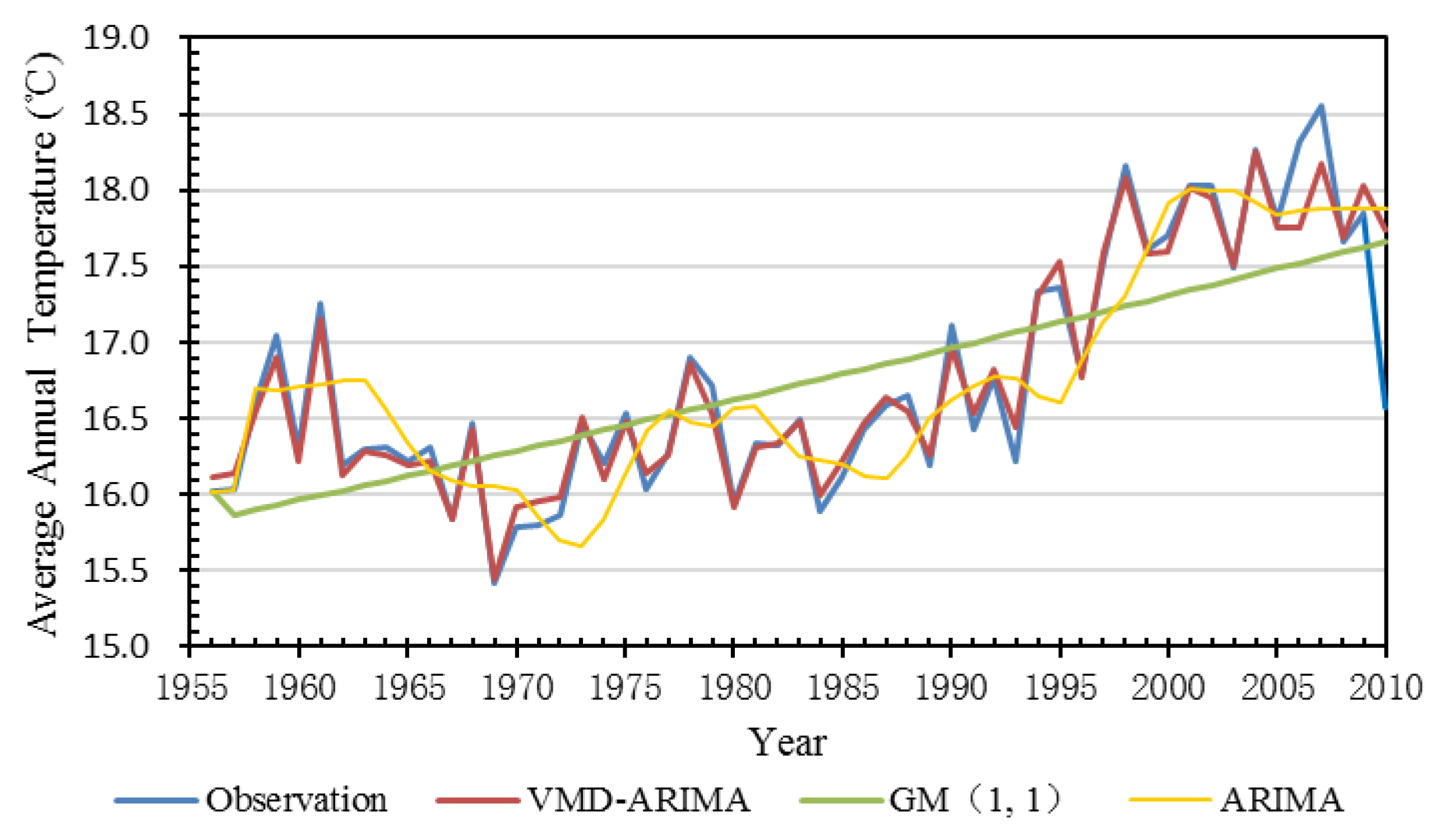
The final forecast results were obtained using the VMD reconstruction of the forecast data of each component model (Figure 4). The forecast values of the average annual temperature from 2006 to 2010 were 17.751 °C, 18.177 °C, 17.687 °C, 18.024 °C, and 17.739 °C, respectively. Overall, the training accuracy was 99.575% and the forecasting accuracy was 97.349%, illustrating the fact that the model is appropriate for fitting and forecasting the average annual temperature. For the performance of the integrated model in different temperature ranges, the model had higher accuracy in years when the temperature changes were moderate. For years with higher temperature fluctuations (such as in 2010), the extent of the fluctuations depicted by the model was much lower than the observed values. Two reasons can be attributed to this phenomenon. First, it could be due to the inherent limitation of the time series model, in which the deterministic trend is expressed by the values of the previous years; therefore, the greater the difference between the current value and the values in the previous years, the greater the difference between the deterministic trend of the model and the observed trend. Moreover, the average annual temperature presented a long-term cycle and a short-term cycle. The correlation between temperatures of different years in the same cycle was weaker than that between temperatures of different years in different cycles. Compared with the transition period of two temperature cycles, the VMD-ARIMA model was, therefore, more suitable for forecasting the average annual temperature in a temperature cycle.
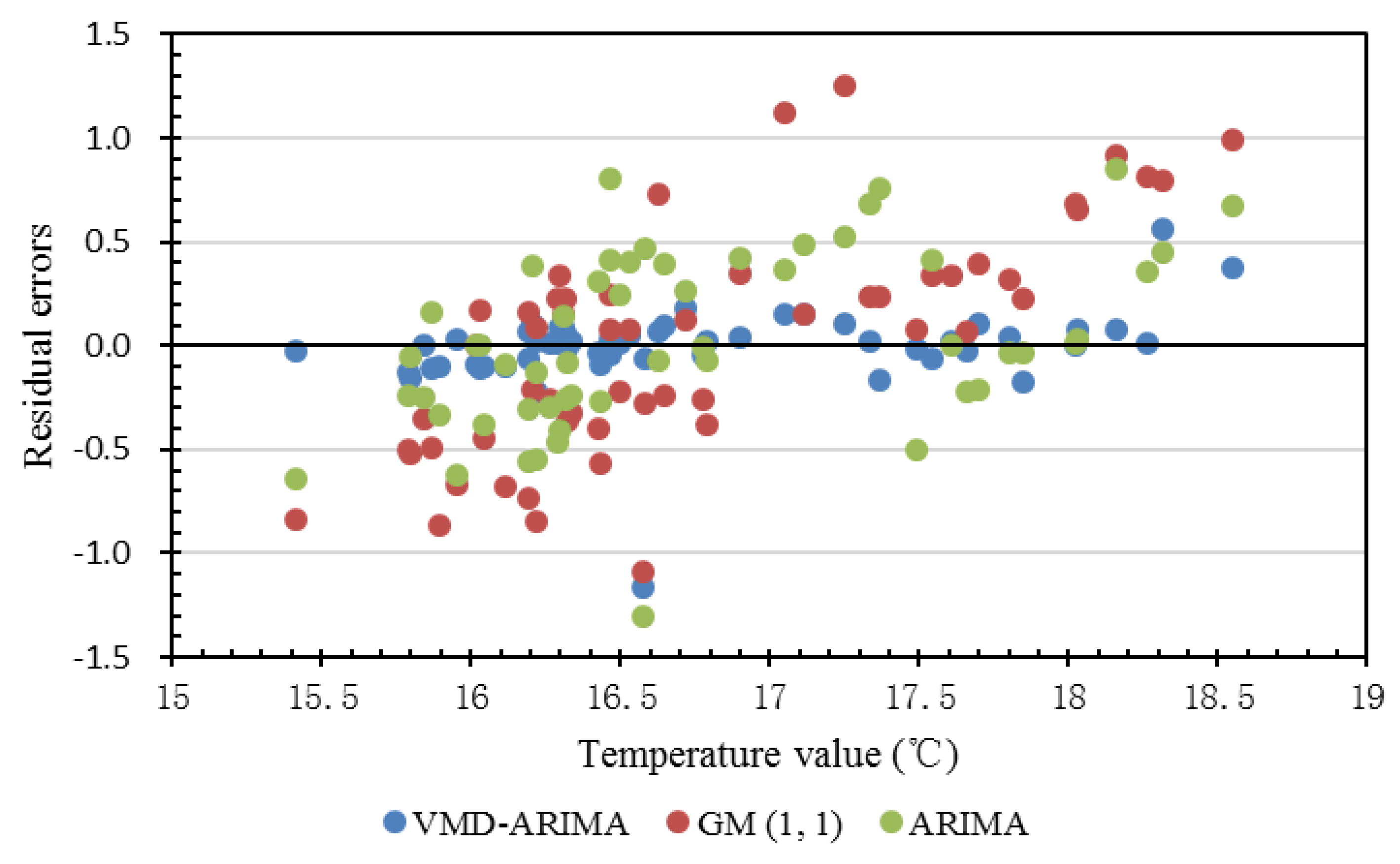
A data sequence without the influencing factors is usually considered as a time series or a grey system. Grey systems theory is a method for studying problems of uncertainty with few data points and poor information. GM (1, 1) is the most commonly used grey model that requires less data; therefore, in order to test the effectiveness of the integrated model, the commonly used GM (1, 1) and the traditional ARIMA model were used on the same data, in which the training samples and the forecasting samples were consistent with the VMD-ARIMA model. The results of the different models are shown in Figure 4. For comparison, the errors of the three models are shown in Table 2, and the residual distributions are shown in Figure 5.
As the ADF value is higher than the t-value with a 5% test critical value, the original data is a non-stationary time series data and the results showed that the three models reflected its overall trend. Nonetheless, for the details of the interannual fluctuations, as can be seen from the residual distribution, the performance of three models were quite different. The residual errors of GM (1, 1) and ARIMA models were higher, and their distributions were more dispersed, while the residual distribution of the VMD-ARIMA model was closer to the zero line. At the same time, the residuals of the GM (1, 1) and ARIMA models in the low and high-value ranges were much larger than the medium range, while the VMD-ARIMA model achieved a better performance in both the middle and low-value ranges. Despite the increase in the error of the VMD-ARIMA model in the high-value range, the error was less than that of the GM (1, 1) and ARIMA models. For the overall training effect, the RMSE of the VMD-ARIMA model was 96.9% lower than that of the GM (1, 1), and 94.9% lower than that of the ARIMA model, indicating that the training effect of the integrated model was much better than the other two models. For the overall forecasting accuracy, the RMSE of the VMD-ARIMA model was 35.5% lower than that of the GM (1, 1) model, and 23.8% lower than that of the ARIMA model. Therefore, the VMD-ARIMA model presented a great improvement in both training and forecasting.
Three main reasons can explain the accuracy improvements: (1) the denoising of VMD, (2) the zero-mean property of the IMF, and (3) the accurate short-term memory of the time series model. The likely cause of the uncertainties in the VMD-ARIMA model was the data preprocessing. During this process, two steps might help contribute to reducing the uncertainties: (1) determining the optimal number of IMF for different data, and (2) smoothing the non-stationary IMF to ensure the stability of each component model. According to the IPCC report [1] and other studies [38,39], global warming on decadal time scales is continuing. Although the time series of regional temperature are different, most of them show similar upward trends with fluctuations [40]. As a result, the trend components of VMD might be similar. The detailed components and optimal numbers of decomposition layers are different. The modeling process is, however, universal and can be applied to different areas.

4. Conclusions

Improving the accuracy of temperature forecasting is an important yet difficult task in current climate change research. In this study, an attempt was made to investigate the performance of a new integrated model, named the VMD-ARIMA, for forecasting annual temperature time series. The VMD-ARIMA model was derived using the average annual temperature data from Wuhan from 1956 to 2005 as a training sample, and the data from 2006 to 2010 as a verifying sample. Three standard statistical performance evaluation measures (MRE, MAE, and RMSE) were adopted to evaluate the performances of the different models. The results indicate that, compared with GM (1, 1) and ARIMA models, the proposed VMD-ARIMA model can better reveal the characteristics of the observations and effectively improve forecasting accuracy. There are several advantages to this integrated model. First, ARIMA forecasting only requires data from the time series in question. Second, the IMF components are more suitable for ARIMA modeling than observations because of their zero mean. Besides, the integrated model can also be applied to other fields with complicated influential factors and obvious time series characteristics, such as meteorology, hydrology, and social economics.
In future studies, we will consider using wavelet analysis to diagnose time series or introduce the weakening operator to correct samples that deviate from the mean. These modifications will help improve the applicability of the model, while also achieving a higher accuracy. In addition, we will try to explore the quantitative response between regional sustainability indicators and temperature changes.

Author Contributions

H.W. and H.Z. conceived and designed the integrated model as well as analyzed the data; H.W. performed the experiments and wrote the paper; J.H. revised the manuscript; L.Z. and Y.Y. contributed materials.

Funding

This research was funded by Changjiang River Scientific Research Institute Open Research Program (CKWV2018499/KY), the Hong Kong Scholars Program (No. XJ201813), and the National Natural Science Foundation of China (No. 41571514).

Conflicts of Interest

The authors declare no conflict of interest.

References

  1. IPCC. Climate Change 2014: Synthesis Report; Core Writing Team, Pachauri, R.K., Meyer, L.A., Eds.; Contribution of Working Groups I, II and III to the Fifth Assessment Report of the Intergovernmental Panel on Climate Change; IPCC: Geneva, Switzerland, 2014; 151p. [Google Scholar]
  2. Clapp, J.; Newell, P.; Brent, Z.W. The global political economy of climate change, agriculture and food systems. J. Peasant. Stud. 2018, 45, 80–88. [Google Scholar] [CrossRef]
  3. Queiros, A.M.; Huebert, K.B.; Keyl, F.; Fernandes, J.A.; Stolte, W.; Maar, M.; Kay, S.; Jones, M.C.; Hamon, K.G.; Hendriksen, G.; et al. Solutions for ecosystem-level protection of ocean systems under climate change. Glob. Chang. Biol. 2016, 22, 927–3936. [Google Scholar] [CrossRef] [PubMed]
  4. Watts, N.; Adger, W.N.; Agnolucci, P.; Blackstock, J.; Byass, P.; Cai, W.; Chaytor, S.; Colbourn, T.; Collins, M.; Cooper, A.; et al. Health and climate change: Policy responses to protect public health. Lancet 2015, 386, 1861–1941. [Google Scholar] [CrossRef]
  5. Kump, L.R. What drives climate? Nature 2000, 408, 651–652. [Google Scholar] [CrossRef] [PubMed]
  6. Gray, L.J.; Beer, J.; Geller, M.; Haigh, J.D.; Lockwood, M.; Matthes, K.; Cubasch, U.; Fleitmann, D.; Harrison, G.; Hood, L.; et al. Solar influences on climate. Rev. Geophys. 2010, 48, 1032–1047. [Google Scholar] [CrossRef]
  7. Wolf, E.T.; Toon, O.B. The evolution of habitable climates under the brightening Sun. J. Geophys. Res.-Atmos. 2015, 120, 5775–5794. [Google Scholar] [CrossRef]
  8. Gattuso, J.P.; Magnan, A.; Bille, R.; Cheung, W.W.L.; Howes, E.L.; Joos, F.; Allemand, D.; Bopp, L.; Cooley, S.R.; Eakin, C.M.; et al. Contrasting futures for ocean and society from different anthropogenic CO2 emissions scenarios. Science 2015, 349, aac4722. [Google Scholar] [CrossRef]
  9. Schuur, E.A.G.; Mcguire, A.D.; Schadel, C.; Grosse, G.; Harden, J.W.; Hayes, D.J.; Hugelius, G.; Koven, C.D.; Kuhry, P.; Lawrence, D.M.; et al. Climate change and the permafrost carbon feedback. Nature 2015, 520, 171–179. [Google Scholar] [CrossRef]
  10. He, J.; Winton, M.; Vecchi, G.; Jia, L.; Rugenstein, M. Transient climate sensitivity depends on base climate ocean circulation. J. Clim. 2017, 30, 1493–1504. [Google Scholar] [CrossRef]
  11. Cai, W.J.; Santoso, A.; Wang, G.J.; Yeh, S.W.; An, S.I.; Cobb, K.M.; Collins, M.; Guilyardi, E.; Jin, F.F.; Kug, J.S.; et al. ENSO and greenhouse warming. Nat. Clim. Chang. 2015, 5, 849–859. [Google Scholar] [CrossRef]
  12. Kirk-Davidoff, D.B.; Schrag, D.P.; Anderson, J.G. On the feedback of stratospheric clouds on polar climate. Geophys. Res. Lett. 2002, 29, 1556. [Google Scholar] [CrossRef]
  13. Roundy, J.K.; Ferguson, C.R.; Wood, E.F. Impact of land-atmospheric coupling in CFSV2 on drought prediction. Clim. Dyn. 2014, 43, 421–434. [Google Scholar] [CrossRef]
  14. Wang, S.J.; Zhang, M.J.; Sun, M.P.; Wang, B.; Huang, X.Y.; Wang, Q.; Feng, F. Comparison of surface air temperature derived from NCEP/DOE R2, ERA-Interim, and observations in the arid northwestern China: A consideration of altitude errors. Theor. Appl. Climatol. 2015, 119, 99–111. [Google Scholar] [CrossRef]
  15. Kay, J.E.; Deser, C.; Phillips, A.; Deser, C.; Phillips, A.; Mai, A.; Hannay, C.; Strand, G.; Arblaster, J.M.; Bates, S.C.; et al. The community earth system model (CESM) large ensemble project a community resource for studying climate change in the presence of internal climate variability. Bull. Am. Meteorol. Soc. 2015, 96, 1333–1349. [Google Scholar] [CrossRef]
  16. Morrison, A.L.; Kay, J.E.; Frey, W.R.; Chepfer, H.; Guzman, R. Cloud response to arctic sea ice loss and implications for future feedback in the CESM1 climate model. J. Geophys. Res.-Atmos. 2019, 124, 1003–1020. [Google Scholar] [CrossRef]
  17. Paulo, A.A.; Ferreira, E.; Coelho, C.; Pereiraa, L.S. Drought class transition analysis through markov and loglinear models, an approach to early warning. Agric. Water Manag. 2005, 77, 59–81. [Google Scholar] [CrossRef]
  18. Ustaoglu, B.; Cigizoglu, H.K.; Karaca, M. Forecast of daily mean, maximum and minimum temperature time series by three artificial neural network methods. Meteorol. Appl. 2008, 15, 431–445. [Google Scholar] [CrossRef]
  19. Ortiz-Garcia, E.G.; Salcedo-Sanz, S.; Casanova-Mateo, C.; Paniagua-Tineoa, A.; Portilla-Figuerasa, J.A. Accurate local very short-term temperature prediction based on synoptic situation Support Vector Regression banks. Atmos. Res. 2012, 107, 1–8. [Google Scholar] [CrossRef]
  20. Ye, L.M.; Yang, G.X.; Van-Rans, E. Time-series modeling and prediction of global monthly absolute temperature for environmental decision making. Adv. Atmos. Sci. 2013, 30, 382–396. [Google Scholar] [CrossRef] [Green Version]
  21. Lee, H.F.; Zhang, D.D.; Fok, L. Temperature, aridity thresholds, and population growth dynamics in China over the last millennium. Clim. Res. 2009, 39, 131–147. [Google Scholar] [CrossRef] [Green Version]
  22. Allen, M.R.; Frame, D.J.; Huntingford, C. Warming caused by cumulative carbon emissions towards the trillionth tonne. Nature 2009, 458, 1163–1166. [Google Scholar] [CrossRef] [PubMed]
  23. Huang, Q.P.; Huang, J.J.; Yang, X.N.; Fang, C.L.; Liang, Y.J. Quantifying the seasonal contribution of coupling urban land use types on Urban Heat Island using Land Contribution Index: A case study in Wuhan, China. Sustain. Cities Soc. 2019, 44, 666–675. [Google Scholar] [CrossRef]
  24. Lei, Y.G.; Lin, J.; He, Z.J.; Zuo, M.J. A review on empirical mode decomposition in fault diagnosis of rotating machinery. Mech. Syst. Signal Process. 2013, 35, 108–126. [Google Scholar] [CrossRef]
  25. McDonald, A.J.; Baumgaertner, A.J.G.; Fraser, G.J. Empirical mode decomposition of the atmospheric wave field. Ann. Geophys. 2007, 25, 375–384. [Google Scholar] [CrossRef]
  26. Wang, N.; Qin, Q.M.; Chen, L.; Bai, Y.B.; Zhao, S.S.; Zhang, C.Y. Dynamic monitoring of coalbed methane reservoirs using Super-Low Frequency electromagnetic prospecting. Int. J. Coal Geol. 2014, 127, 24–41. [Google Scholar] [CrossRef]
  27. Mert, A. ECG feature extraction based on the bandwidth properties of variational mode decomposition. Physiol. Meas. 2016, 37, 530–543. [Google Scholar] [CrossRef] [PubMed]
  28. Long, J.; Wang, X.; Dai, D.; Tian, M.; Zhu, G.; Zhang, J. Denoising of UHF PD signals based on optimised VMD and wavelet transform. IET Sci. Meas. Technol. 2017, 11, 753–760. [Google Scholar] [CrossRef]
  29. Dou, C.; Zheng, Y.; Yue, D.; Zhang, Z.; Ma, K. Hybrid model for renewable energy and loads prediction based on data mining and variational mode decomposition. IET Gener. Transm. Distrib. 2018, 12, 2642–2649. [Google Scholar] [CrossRef]
  30. Dragomiretskiy, K.; Zosso, D. Variational mode decomposition. IEEE Trans. Signal Process. 2014, 62, 531–544. [Google Scholar] [CrossRef]
  31. Box, G.E.P.; Jenkins, G.M. Series Analysis Forecasting and Control, 1st ed.; Holden-Day: San Francisco, CA, USA, 1976. [Google Scholar]
  32. Valipour, M.; Banihabib, M.E.; Behbahani, S.M.R. Comparison of the ARMA, ARIMA, and the autoregressive artificial neural network models in forecasting the monthly inflow of Dez dam reservoir. J. Hydrol. 2013, 476, 433–447. [Google Scholar] [CrossRef]
  33. Valipour, M. Long-term runoff study using SARIMA and ARIMA models in the United States. Meteorol. Appl. 2015, 22, 592–598. [Google Scholar] [CrossRef]
  34. Shukur, O.B.; Lee, M.H. Daily wind speed forecasting through hybrid KF-ANN model based on ARIMA. Renew. Energy 2015, 76, 637–647. [Google Scholar] [CrossRef]
  35. Yuan, C.; Liu, S.; Fang, Z. Comparison of China’s primary energy consumption forecasting by using ARIMA (the autoregressive integrated moving average) model and GM (1, 1) model. Energy 2016, 100, 384–390. [Google Scholar] [CrossRef]
  36. Boroojeni, K.G.; Amini, M.H.; Bahrami, S.; Iyengar, S.S.; Sarwat, A.I.; Karabasoglu, O. A novel multi-time-scale modeling for electric power demand forecasting: From short-term to medium-term horizon. Electr. Power Syst. Res. 2016, 142, 58–73. [Google Scholar] [CrossRef]
  37. Romilly, P. Time series modelling of global mean temperature for managerial decision-making. J. Environ. Manag. 2005, 76, 61–70. [Google Scholar] [CrossRef] [PubMed]
  38. Hansen, J.; Ruedy, R.; Sato, M.; Lo, K. Global Surface Temperature Change. Rev. Geophys. 2010, 48, RG4004. [Google Scholar] [CrossRef]
  39. Hansen, J.; Sato, M.; Ruedy, R.; Lo, K.; Lea, D.W.; Medina-Elizade, M. Global temperature change. Proc. Natl. Acad. Sci. USA 2006, 103, 14288–14293. [Google Scholar] [CrossRef] [Green Version]
  40. Hansen, J.; Sato, M. Regional climate change and national responsibilities. Environ. Res. Lett. 2016, 11, 034009. [Google Scholar] [CrossRef] [Green Version]
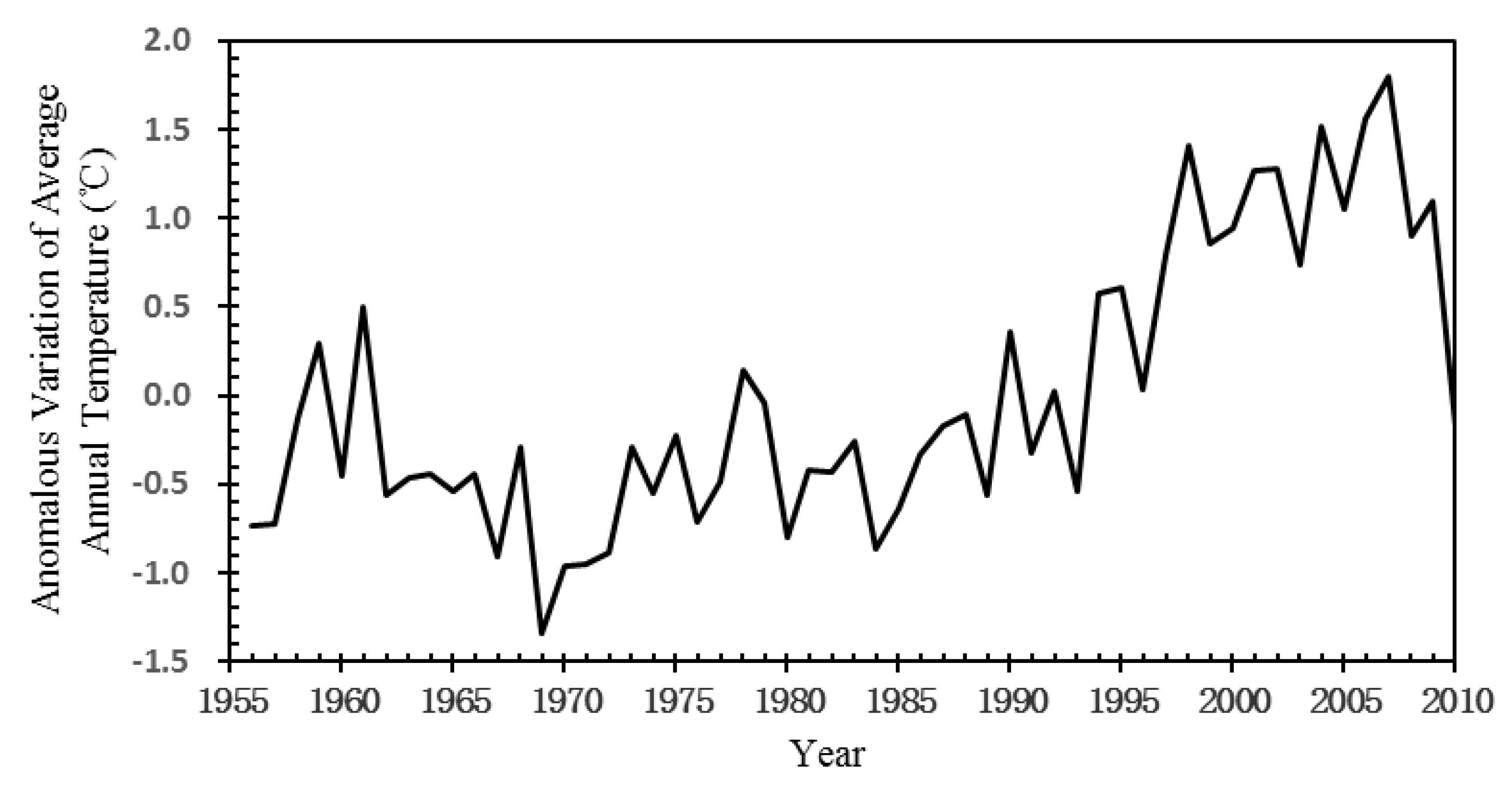
Figure 1. Anomalous variation of average annual temperature during 1956–2010.
Sustainability 11 04018 g001
Figure 2. Observation and VMD components.
Sustainability 11 04018 g002
Figure 3. Comparison of forecast values and observations of component models.
Sustainability 11 04018 g003
Figure 4. Results of the VMD-ARIMA model, GM (1, 1), and ARIMA model.
Sustainability 11 04018 g004
Figure 5. Residual errors of the VMD-ARIMA model, GM (1, 1), and ARIMA model.
Sustainability 11 04018 g005
Table 1. Adopted structure and parameters of ARIMA.
ComponentModel Structure φ i θ j A I C Adjusted R2
RESARIMA (4, 1, 6)−0.070, −0.435, 0.678,2.267, 3.870, 4.378−5.7710.975
−0.0133.667, 2.002, 0.861
IMF1ARIMA (4, 0, 6)0.467, −1.079, 0.378,0.076, −0.886, 0.341−3.0160.932
−0.5210.737, −0.731, −0.460
IMF2ARIMA (3, 0, 2)−0.975, 0.209, 0.551−1.051, 0.088−3.4960.959
Table 2. Errors of the VMD-ARIMA model, GM (1, 1), and ARIMA model.
ModelTrainingForecasting
MREMAERMSEMREMAERMSE
GM (1, 1)0.0250.4180.2560.0360.6340.572
ARIMA0.0200.3320.1570.0310.5380.484
VMD-ARIMA0.0040.0700.0080.0270.4610.369