This section describes the analysis of the transport energy consumption per capita of the investigated cities. In a first step, the transport energy of cities is calculated as precisely as possible from the collected data. Thereafter, the transport energy is modeled based on infrastructure accessibility and population density.
3.1. Transport Related Energy Consumption
Considering the available data, the most precise estimate of the transport energy per person per year for commuting purposes
in city
i the can be determined by:
where
is the share of working population of the total population,
is the daily average commuting distance to work by private car,
is the daily average commuting distance to work by public transport,
is the mode share of private car trips,
is the mode share of trips with public transport,
is the average energy consumption per person km for a private car,
is the average energy consumption per person km for public transport and one year corresponds to 261 working days.
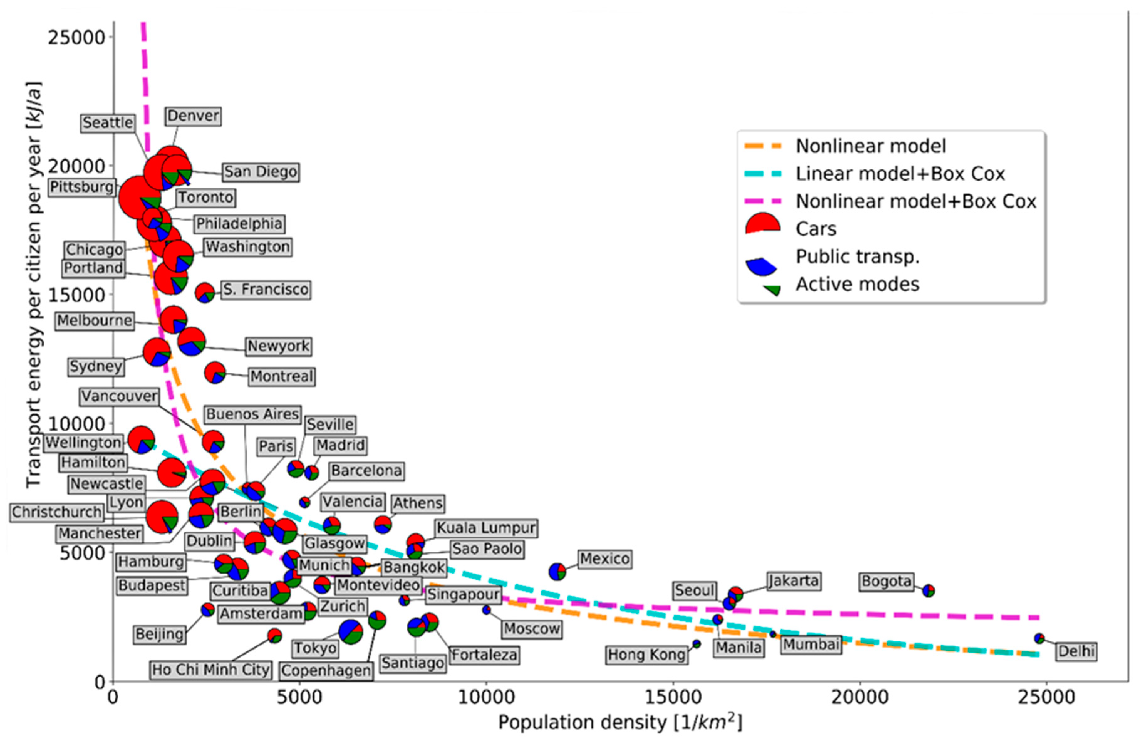
Figure 1 shows the transport energy
WT and mode share versus the population density for each city. The same figure contains the hyperbolic shape of
WT, which is similar to Newman and Kenworthy’s curve. A cluster of cities can be seen at low population densities between 1000–2500 persons/km
2, where the majority are U.S. and Canadian cities. These low population density cities are showing a much higher transport related energy consumption compared with cities with higher population density. Low population density cities are also characterized by a high road infrastructure accessibility (see diameter of bubbles in
Figure 1) and high car mode share (see pie chart of bubbles in
Figure 1). Regarding mode shares of daily commuting in the U.S.: the private vehicle mode share is over 85% of all trips, which is followed by 5.2% share of public transportation trips [
26]. Canadian, Australian and New Zealand cities, where car dependent mobility concepts are adopted, have, on average, slightly lower road infrastructure accessibility and slightly higher public transport usage compared with U.S. cities.
A cluster with mainly European, Latin American cities and some Asian cities such as Tokyo can be seen at population densities between 2500–8000 persons/km2 with medium level road infrastructure accessibility. Cities in this cluster consume noticeably less transport energy with respect to the first cluster. It is apparent that in this cluster, cities with the highest active mode share such as Tokyo, Amsterdam and Copenhagen consume the lowest transport energy. The cluster of cities with population densities above 8000 persons/Km2 are mainly Asian cities with low road infrastructure accessibility and a high public transport share.
The particularly sharp rise in energy consumption for decreasing population densities calls for some reasoning. The non-linear model shown in
Figure 1 is developed in the following section.
3.2. Transport Infrastructure Population Density and Transport Energy Consumption
This section investigates how transport infrastructure and population density determine transport energy consumption, estimated in Equation (1). The road infrastructure accessibility (RIA) and other infrastructure accessibilities (rail-track infrastructure accessibility TIA and bike infrastructure accessibility BIA, which can be calculated with OSM data) are assumed to have an impact only on the respective mode shares MSC, MSPT and MSA, not on the other variables in Equation (1). The energy efficiency of private and public transport will not be part of the modeling.
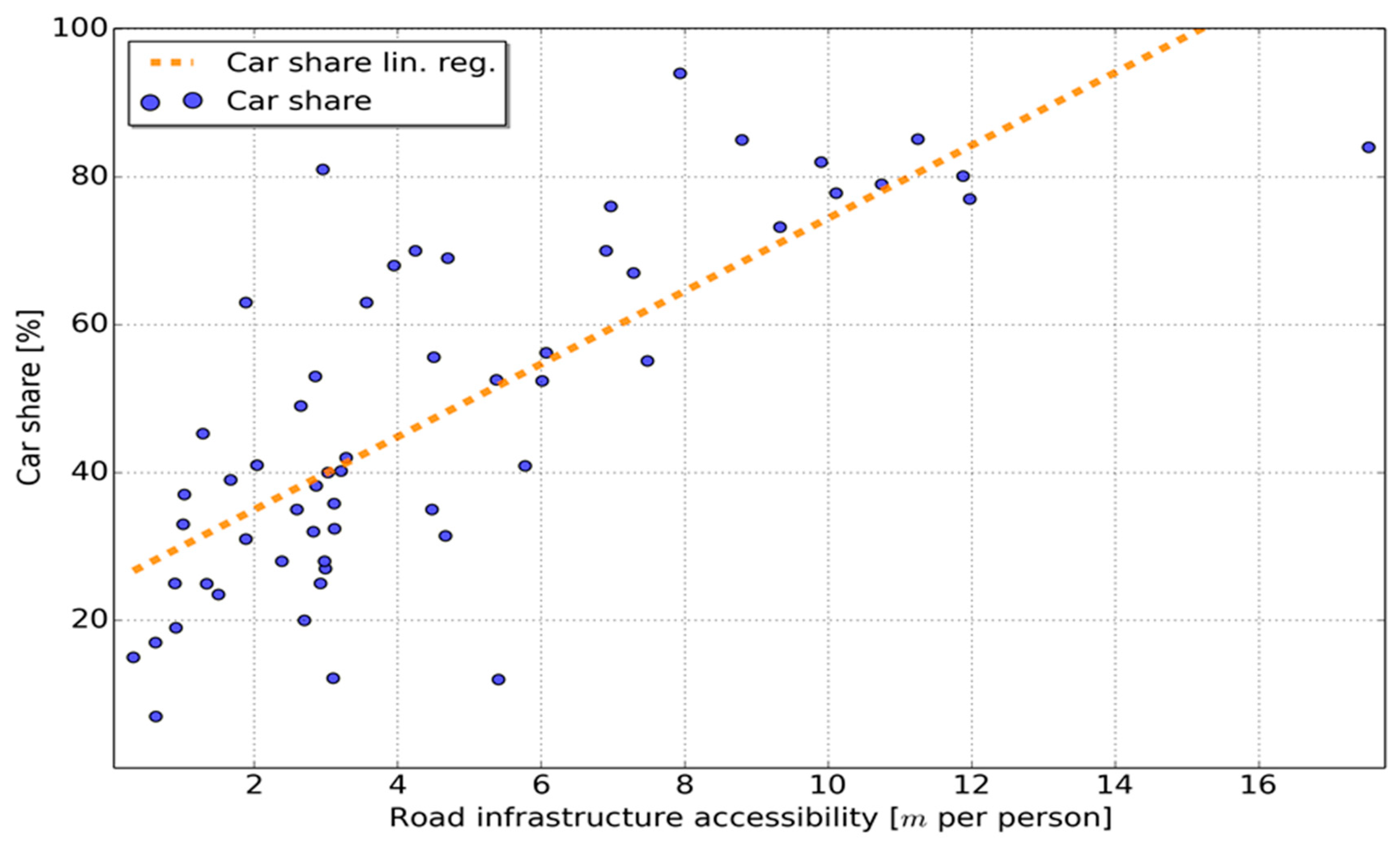
Concerning the MSC, the data shown in
Figure 2 suggests a linear relation between road infrastructure accessibility RIA and car mode share MSC. The MSC has been estimated with the following equation:
where parameters have been estimated with a linear regression, see
Table 1. The fit with
is relatively good, considering the different error sources in the determination of RIA and MSC. The Harvey Collier test resulted in a p-value of 0.41, confirming that the null hypothesis that linear specification is correct should not be rejected. The skew is close to zero (0.198) and the p-value of the Jarque-Bera test is 0.62, indicating normally distributed residuals, even though there are uncertainties due to the small sample number. However, the reason why the road length per inhabitant increases car mode share in proportional way is not clear. In the literature, similar relations have been demonstrated empirically [
6,
7].
Regarding the public transport mode share MSPT, it is more difficult to establish a relation between the rail track length per inhabitant TIA and MSPT in the absents of more detailed information: the rail length represents only a part of all public transport infrastructures and in any case, the rail usage is only a share of all public transport trips. One interesting possibility is to test whether the MSPT depends also on the road infrastructure. Indeed, the linear approach has been tested:
with regression parameters
and
shown in
Table 2. The results show that RIA is significant, and as
is negative, an increasing RIA decreases public transport mode share, as expected. With
the fitting is less pronounced with respect to Equation (2). The linear specification is correct as the p-vale of the Harvey Collier test equals 0.55 and it is likely that the residuals are normal distributed due to a skew close to zero and a Jarque-Bera
p-value of 0.26.
Further modeling showed that also the bike mode share is negatively correlated with RIA.
The population density is assumed to influence the average daily commuting distances by car, DC, and the average daily commuting distances by public transport, DPT. The linear regression model:
shows that DC decreases with an increasing population density, parameters are statistically significant, but the fit is very weak as
, see
Table 3. The linear specification is correct as the p-vale of the Harvey Collier test equals 0.92. The residuals are likely to be normal distributed due to a skew close to zero (0.165) and a Jarque-Bera p-value of 0.77. The parameter
has a relatively low absolute value, which means commute distances are slightly sensitive to the population density. The influence of the population density on the PT commute distance is not statistically significant for the present dataset.
Considering solely road infrastructure accessibility RIA and population density DPOP as independent variables, the transport energy estimate
of a generic city shall be estimated by substituting the estimates of models from Equations (2)–(4) in the energy equation of Equation (1). The resulting energy estimate can be presented in the shape:
where the following parameters are assumed to be constant and independent from
DPOP and
RIA:
Note that the city index
i of the various parameters in Equation (1) has been dropped and the respective quantities have been replaced by average values. The beta parameters in Equation (5) are determined by a linear regression instead of using the above equations, because doing so would lead to multiplicative errors. The regression results are presented in
Table 4. This estimate is fitting well with the energy data as
, and the signs of the parameters meet expectations. However, the parameter
related to DPOP is not statistically significant and takes positive values within the 95% confidence interval. In addition, the independent variables are not homoscedastic as the p-value of the Breusch-Pagan Lagrange Multiplier test is a low
A Box-Cox transformation of the model with the optimal lambda value of
−0.036 is not able to improve this condition.
Dropping the explicit dependency on DPOP from Equation (5), one ends up with the simple transport energy estimate:
with the parameters
and
to be calibrated. However, as demonstrated below, RIA does depend on DPOP. The regression results in
Table 5 demonstrate that both parameters are significant, with
, which is only little worse than the model in Equation (5). The linear specification is correct as the p-vale of the Harvey Collier test equals 0.30. However, the residuals are unlikely to be normal distributed as the skew is different from zero (0.712) and the Jarque-Bera
p-value is 0.012, which is below 0.05.
Any attempts to include rail-track infrastructure accessibility or bike infrastructure accessibility in the transport energy estimation resulted in a better fit of the energy data, but statistical significance is lacking.
3.3. The Relation between Population Density and Transport Energy Consumption
There still needs to be an explanation as to why the transport energy per person shown in
Figure 1 is increasing so sharply for low population density. The previous section shows that the average travel distance DC is little sensitive to DPOP. Therefore, it must be the private car mode share MSC that increases in a non-linearly fashion as DPOP approaches zero. However, if the MSC increases linearly with RIA, as demonstrated in
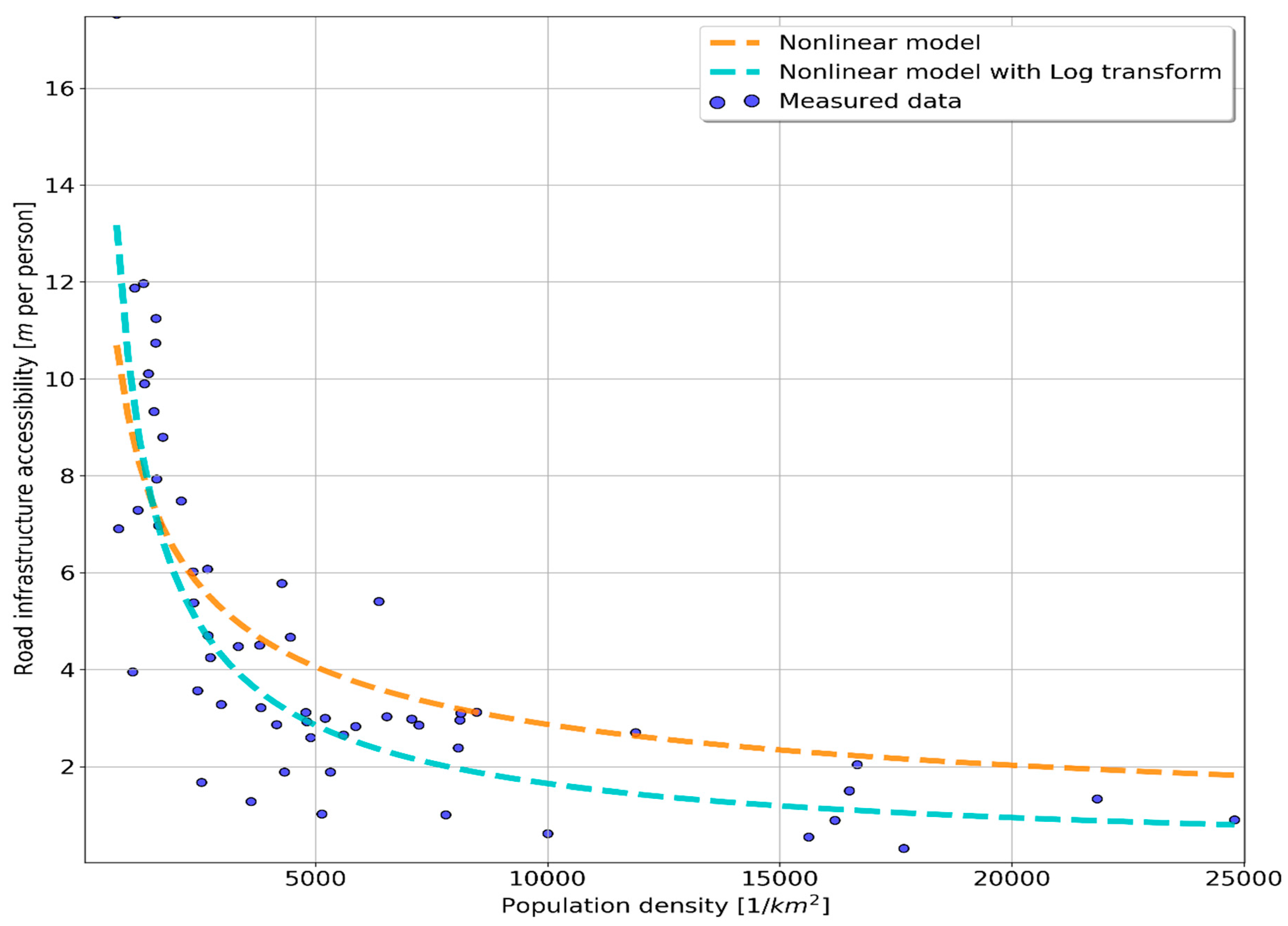
Section 3.1, then the relation between DPOP and RIA is necessarily of non-linear nature. In fact,
Figure 3 shows that the RIA of the cities is rapidly decreasing as DPOP increases, similar to the transport energy curve in
Figure 1.
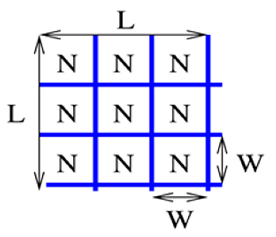
The following approximations are an attempt to explain why the road length per person tends to increase so dramatically for cities with low population density: assuming a city with a squared layout with side length
L and a grid-like road network where all streets are
W meters apart, as shown in
Figure 4, of which the number of roads is
in each coordinate and the total road length is
.
Assuming further that the population is evenly spread over the city, then the population density is
and the total population becomes
As the road infrastructure accessibility is defined by
,
RIA is obtained by replacing
W with
:
where
can be seen as a constant to be calibrated. Clearly, this equation determines the road length of a cities with varying population density, while limiting the road circuity constant to
, which is a typical value for U.S. cities [
39]. Note that
RIA is dropping sharply for increasing
DPOP, as expected from the city data. Applying an ordinary linear regression on the city data with DPOP in inhabitants per m
2, the term
is found to be statistically significant and within 0.256 and 0.316, using the 95% confidence interval. The average value of
. Despite the simplicity of the grid-road model city, the estimate shows a goodness of fit with
, even though the residuals are unlikely to be normal distributed as the skew is different from zero (0.856) and the Jarque-Bera
p-value far below 0.05. The linear specification is correct as the p-vale of the Harvey Collier test equals 0.92.
It is worth mentioning that the estimate fits well because the calibration is determined by U.S. cities with a large RIA at low population densities and Asian cities with low RIA and high population densities, and just those dominant U.S. cities are the ones best represented by the regular road-grid that has been assumed in the above model.
The result of Equation (7) shall be verified by calibrating a non-linear model with a generic exponent
of the shape:
and by comparing
with the exponent 0.5 in Equation (7). With a log transformation, this problem can be transformed in a linear estimation problem of the form:
where
and
. The regression results of the log-model in Equation (9) are shown in
Table 6. The linear specification is correct as the p-vale of the Harvey Collier test equals 0.24. However, the residuals are unlikely to be normal distributed as the skew is different from zero (−0.945) and the Jarque-Bera p-value well below 0.05.
Apparently, the exponent
= 0.78 from Equation (8) is different from the exponent value of 0.5 in Equation (7), which represents the square root. Moreover,
= 0.44 is different but in the same order of magnitude than
from Equation (7). The goodness of fit of the model in Equation (8) with
is marginally higher with respect to the model in Equation (7). These minor differences are not surprising, given the simplifying assumptions made during the derivation of Equation (7). The results of the two models are plotted in
Figure 3.
As the derived model in Equation (7) reasonably explains the
RIA of cities, Equation (7) is substituted into the energy estimate of Equation (6), which leads to a transport energy model as a nonlinear function of the population density. The shape of this transport energy estimate becomes:
with the parameters
and
to be calibrated with the transport energy data. The linear regression results in
Table 7 indicate that both parameters are significant, the sign of
is positive, as expected, and the fit is reasonable with
. The linear specification is correct as the
p-vale of the Harvey Collier test equals 0.24. The residuals are likely to be normal distributed due to a skew close to zero (−0.128) and a Jarque-Bera
p-value of 0.41. This estimate explains the sharp rise of transport energies for low-density cities as previously shown in
Figure 1.
In order to judge whether the particular non-liner shape of the model in Equation (10) is a reasonable fit, two other modeling attempts are investigated: first, a linear Box-Cox model of the form:
has been calibrated with an optimal
. The parameters from Equation (11) are shown in
Table 8. The outcome of the linearity test and the normal distribution test are equivalent to the results of the non-linear model from Equation (10). After a back-transformation of Equation (11), the obtained goodness of fit equals
.
In a second attempt, a Box Cox transformed model with a non-linearity in
has been calibrated, similar to the one in Equation (10):
With the previously optimized
, the parameters from Equation (12) are shown in
Table 9. The outcome of the linearity test and the normal distribution test are again identical to the non-linear model from Equation (10). After a back-transformation, the goodness of fit showed results in
.
Apparently, the model in Equation (10) does best fit with the measured energy data. All three models of the transport energy estimation are shown in
Figure 1.
3.4. Summarizing Discussion
Two quantities have been investigated, which can significantly influence the transport energy of cities, see Equation (1): the modal split and the average commute distance. From the present city dataset, there is statistical evidence that private commute travel distance is linearly decreasing with population density, see Equation (4). The model shows a ratio of approximately 50% between the commute distance of cities with highest and lowest population densities. However, the errors of this distance model are fairly large.
Regarding the mode shares, a significant, linear relation has been found between road infrastructure accessibility (RIA) and car mode share (MSC), see Equation (2). In this case, the ratio between MSCs of cities with the lowest and highest RIA is approximately 400%. This result means that RIA has a much stronger influence on the mode share than the population density has on the commute distance. The public transport infrastructure can only be represented by the rail length extracted from the OSM data of each city. This information proves insufficient to establish a relation between public transport infrastructure and public transport mode share MSPT, as rail constitutes only a part of all public transport trips. Instead, it has been possible to demonstrate that MSPT is decreasing linearly with RIA. The linear relations between RIA, MSC and MSPT have only been demonstrated empirically and a model to explain this relation quantitatively has not been found in literature. Nevertheless, as RIA does determine significantly both shares, MSC and MSPT, the transport energy has been estimated with a linear regression that depends only on RIA, see Equation (6). The failed attempts to include rail infrastructure accessibility (TIA) or bike infrastructure accessibility (BIA) in the transport energy estimation is probably due to the fact that both OSM data are insufficiently precise or incomplete to explain the public transport or active mode share, respectively. However, including rail and bike infrastructure accessibility reduces the errors in the model. Further tests have revealed that TIA actually increases proportionally with the rail mode share (for 17 cities,
) and BIA is proportional to bike mode share (for 32 cities,
). These findings support the relation between usage and alternative infrastructures expansion presumably by shifting car trips to alternative modes, as demonstrated in [
43,
44,
45] for rail and in [
46,
47] for cycling. Better fits can be obtained when concentrating on a particular area: for example, the relation between BIA and the bike mode share has a better fit using only European cities with respect to cities from all countries available in the database. Still, the active-mode share includes walk-trips and walk infrastructure is difficult to assess with OSM data as footpath are generally insufficiently modelled in OSM.
In
Section 3.2, a non-linear function between the population density and RIA has been derived from the data, based on a simplifying road-grid model, see Equation (7). This calibrated model fits well with empirical population density and RIA data and shows a marked rise of RIA as population density approaches zero. This model has been verified by calibrating a more generic model, whose parameters relaxed to values similar to the derived model of Equation (7). Combining the function in Equation (7) to compute RIA from the population density with the linear relation from Equation (6), which estimates the transport energy, it has been possible to calibrate a statistically significant model that estimates the transport energy as a function of the population density, see Equation (10). This model can explain the marked rise in transport energy for cities with low population density, as found already by Newman [
5]. Nevertheless, there are some cities that do not fit well with the estimated energy curve: Hamilton, New Zealand, has a high car mode share (94%), but a relatively low energy use for its low population density. The reason is Hamilton’s relatively low average commute distance. Moreover, Ho Chi Minh City has short commute distances and, therefore, a relatively low transport energy consumption. Wellington has a low energy consumption for its population density, but as the metropolitan area has been used, the population density might be underestimated as most of the population lives in Wellington city. The Spanish cities Madrid, Seville and Barcelona have a relatively high transport energy consumption, despite a low car mode share, due to an exceptionally high commute distance.
Attempts to include the average commute distance as a linear function of the population density resulted in a slightly improved fit of the transport energy, but parameters became statistically insignificant and are not suited to explain the phenomenon.


