Article

Optimal Sizing of Irregularly Arranged Boreholes Using Duct-Storage Model

Division of Architecture, INHA University, Inha-ro 100, Michuhol-gu, Incheon 22212, Korea
*
Author to whom correspondence should be addressed.
Sustainability 2019, 11(16), 4338; https://doi.org/10.3390/su11164338
Submission received: 18 July 2019 / Revised: 1 August 2019 / Accepted: 8 August 2019 / Published: 11 August 2019

Abstract

:
As the sizing of borehole heat exchangers (BHEs) is crucial for ground-source heat pump systems, which are becoming increasingly complex and diverse, novel sizing tools are required that can size both boreholes and connected systems. Thus, an optimization-based sizing method that runs in TRNSYS with other component models is proposed. With a focus on the feasibility of the method for typical BHEs, the sizing of irregularly placed boreholes using the well-known duct-storage (DST) model that inherently cannot describe irregular borefields is examined. Recently developed modification methods are used for the DST model. The proposed sizing method is compared with the existing ground loop heat exchanger (GLHE) sizing program. The results indicate that the proposed method has a genuine difference of approximately 3% compared with the GLHE, and the difference increases with the thermal-interference effects. A regression-based method selected to modify the DST model for describing irregular borefields exhibits acceptable sizing results (approximately 5% for test cases) despite the genuine difference. This study is the first to use the DST model for sizing BHEs under irregular borefield configurations, and the tests indicated acceptable results with an approximate difference of one borehole among a total of 30 boreholes in the test cases.

1. Introduction

Ground-source heat pump (GSHP) systems generally consist of a load-side loop, heat pumps, and source-side ground heat exchangers (GHEs). Among the different types of GHEs, vertically installed borehole heat exchangers (BHEs) are commonly used in GSHP systems [1,2]. BHEs are usually installed in the ground with a depth of 100–250 m for exploiting the reduced fluctuations in the ground temperatures over years. GSHP systems extract heat from the ground and transfer it to a building via the BHEs in the heating period, whereas heat is injected into the ground during the cooling period.
As the ground temperatures gradually increase or decrease over years according to the load patterns, adequate sizing of BHEs is crucial for ensuring the high efficiency of the GSHP. For instance, undersized BHEs cause poor system performance or even system failure, and oversized BHEs incur high initial costs. Adequate sizing may ensure the long-term performance of the whole GSHP system. Generally, the sizing of BHEs is achieved using commercial design programs such as GLD [3], ground loop heat exchanger (GLHE)- [4], and EED [5]. Possible results obtained from these tools are the total required lengths, entering water temperatures (EWTs) to the heat pumps after a certain period, and the approximate heat-pump energy consumption. As building systems have recently become increasingly complex and diverse, the sizing of BHEs has become more sophisticated [6,7,8,9,10]. Thus, there is a need for novel design methods that are capable of sizing both boreholes and connected systems simultaneously. Dynamic simulation-based sizing methods have attracted attention. TRNSYS [11], which is a well-known commercial dynamic simulation tool, can be used for this purpose. An advantage of TRNSYS is that its library includes various building system component models, most of which have been developed and validated through numerous research and engineering projects. Among them, the Type 557 duct-storage (DST) model is included, which can simulate borefields and has been extensively used [11]. Additionally, TRNOPT—an optimization tool—can be easily implemented in the program. As shown in Table 1, several studies pertaining to the optimization of GSHP systems have been performed using TRNSYS with the DST model. Most of the studies were performed to optimize not only the length of the BHEs but also the system variables, such as the flow rates, capacities of the combined systems, and materials.
The DST model was developed by Hellström in the late 1980s to model borehole thermal energy storage (BTES) systems [12]. This model assumes three-dimensional heat transfer around boreholes according to a two-dimensional axisymmetric case using the cylindrical coordinate system (r, z). Consequently, computation with the DST model is rapid; thus, the model has been extensively used for optimization problems that require several iterative calculation loops. However, the reduction in the dimension limits the use of the model to regular arrangements of BHEs. This is acceptable for the BTES, but the model is not useful for common GSHP systems installed in buildings, where the BHEs are placed around the building. For this reason, researchers have developed custom models to simulate irregular BHE configurations [7,13] in three-dimensional grids, despite the significantly increased calculation time.
However, studies have suggested that the DST model can describe some irregular configurations through modification of the main parameters [18,19,20]. It is impossible to explicitly adopt a user-defined configuration in the DST model, but optimized parameters can exhibit similar thermal dynamics for some typical arrangements that are commonly found in GSHP systems. For instance, I, L, U, and hollow-rectangular-shaped configurations were examined in previous studies [19,20]. In the present study, these modification methods were reviewed, and they were combined with the proposed optimization sizing method to examine the sizing results compared with those of an existing design tool. Until now, no studies have employed the DST model for sizing irregular borefields.
In the following sections, the modification methods are briefly described, and the sizing method with optimization is proposed. Then, the sizing results of the proposed method are compared with those of an existing sizing software for the cases that were used in development of the modification method as well as other cases.

2. Review of Modified DST Models
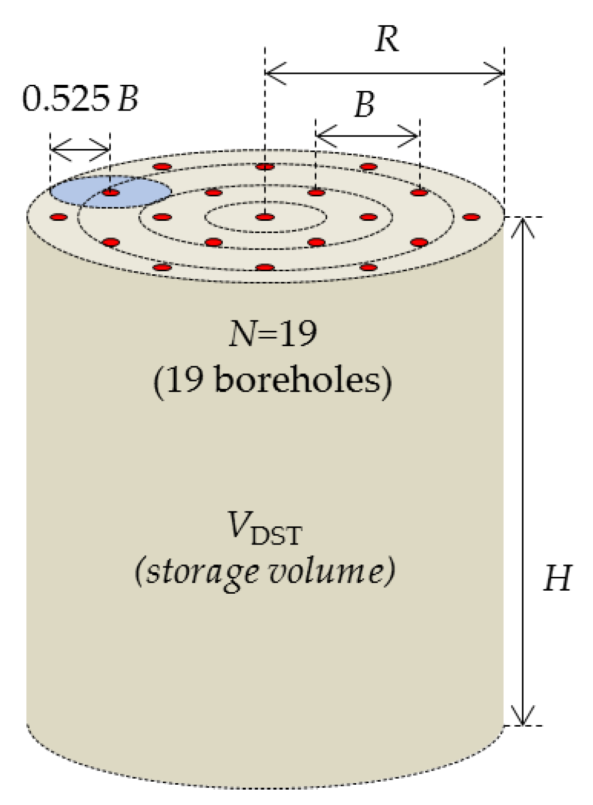
2.1. DST Model

The DST model was developed by Hellström [12] and was implemented in TRNSYS by Pahud [21]. Currently, the DST model is included in the TESS library, which is an advanced full library of TRNSYS. The DST model can analyze the heat transfer from the BHE to the ground for a single BHE or multiple BHEs. In the DST model, the borefield is cylindrically configured, and the distances among the BHEs are assumed to be uniform, as shown in Figure 1 [22,23]. Figure 1 shows a configuration where 19 boreholes are regularly arranged in the ground heat storage volume of the DST model. If users set the number of BHEs (N), borehole spacing (B), and buried depth (H), the BHEs are automatically placed in the cylindrical volume called the storage volume (VDST).
C T t = · ( λ T ) + q sf + q
Calculations in the DST model is executed on the three parts; global, local, and steady-flux problems. Equation (1) shows the fundamental heat transfer in the global part of the DST model with two heat source terms, qsf, q. Here, qsf represents heat energy redistribution due to the circulation of working fluid, and this is assumed as a steady-flux problem. q indicates heat transferred from the local to the global problem. For the global and local problem, the explicit finite-difference method (FDM) is used whereas the steady-flux problem adopts an analytical solution. The global problem covers the large-scale thermal volume from the heat storage to the surrounding ground using two-dimensional grids while the individual BHEs are left to the steady-flux and local problems assuming one-dimensional heat transfer [12].
As mentioned previously, one feature of the DST model is that the arrangement cannot be changed by users. Thus, the DST model is typically used for simulations of BTES systems [24,25,26] or GSHP systems with a small number of BHEs, where the arrangement is relatively unimportant for low thermal-interference effects among the BHEs [12,27].
The VDST parameter is defined by Equation (2). The individual volume for each BHE is approximately equal to that of a small cylinder with a radius of 0.525 B and a height of H. In previous studies, this parameter was modified to describe irregular borefields.
VDST = π × H × N × (0.525B)2

2.2. Modified DST Models

2.2.1. Rule-Of-Thumb Modification

Bertagnolio et al. [18] introduced the possibility that a modified VDST can describe irregular borefield cases. They proposed changing VDST for an I-shaped arrangement (8 × 1). They compared borehole wall temperatures obtained using this modification of the DST model with those obtained using Eskilson’s g-function [28], and results indicated a difference of <0.6 °C. In their study, VDST was re-defined using a new radius (R) such that the new cross-sectional perimeter, 2πR, was equal to the I-shaped borefield perimeter, 2 × (N × B + B). Thus, the resulting modified VDST was significantly larger than the previous cylindrical volume. Accordingly, the equivalent borehole spacing increased for the I-shaped borefield. This can be explained by the fact that the thermal interferences between the BHEs become stronger in the dense regular configuration shown in Figure 1. The boreholes in the center experience thermal interference from six adjacent boreholes, while the boreholes along the rim are affected by three or four adjacent boreholes. In contrast, in the I-shaped arrangement, each borehole is affected by only two adjacent boreholes.
Based on this idea, Park et al. [19] proposed a rule-of-thumb formula that is applicable to I, U, L, and hollow-rectangular (Rec) borefields, as shown Equation (3). In order to utilize the DST model for typical borefield cases, they selected common BHE configurations irregularly placed with a uniform spacing among adjacent boreholes. They assumed that the borefields consist of multiple I-shaped sub-groups. Here, the lowercase letter s represents the number of I-shaped borefields; the I, L, U, and Rec shapes have values of 1, 2, 3, and 4, respectively. All the sub-group I-shaped borefields are included in a single DST model; hence, this model can account for the thermal-interference effects among the I-shaped sub-groups.
VDST,modif.V1 = s × π × H × [{(NB/s) + B}/π]2,
Equation (3) was compared with a reference model for the L-shaped 19-BHE case, and the difference between the highest EWTs after a simulation of 20 years was 0.52 °C [29].

2.2.2. Regression-Based Modification

Park et al. [20] performed a more detailed analysis to propose a new modification method. They quantified the thermal-interference levels in a specific borefield using the measured mean total distances (S) from one borehole to all the other boreholes. Therefore, any user-defined irregular borefield can be specified by Stest. In their study, a reference value of SDST was used, which represented the mean total distance (S) of a borehole when the same number of BHEs were placed in the DST manner, maintaining the spacing among adjacent BHEs. The ratio of Stest/SDST was used as a variable to develop a regression model for setting a new borehole distance (B’), as shown in Table 2. Toward the I-shape, the equivalent borehole spacing (B’) becomes larger, as Stest/SDST is also larger. Park et al. [20] used the optimization algorithm to quantify , and a hybrid-reduced (HR) model [30] was used to identify the optimal coefficients of Equation (4) such that the mean EWT of the DST model was close to the mean value of the HR model for 10 years. Numerous values were evaluated for 36 BHE configuration cases related to the Rec-, U-, L-, and I-shaped configurations, and the correlated coefficients were obtained, as shown in Table 3. This modification of the storage volume in the DST model is presented in Equation (5).
= b0 + b1X1 + b2X2 + b3X3 + b4X4 + b5X5,
Using the in Equation (4), another modified VDST was obtained, as follows:
VDST, modif.V2 = π × H × N ×(0.525B’)2
This regression-based modification method approximated the EWT within a mean difference of 0.5 °C compared with the referenced HR model [30] when the annual ground loads were neither highly heating- nor cooling-dominant. The model was only validated for cases where Stest/SDST was smaller than 5.5 [20]. The borefield configurations shown in Table 2 were selected to cover BHE configurations found in common GSHP projects, and similar borefields are used in this work to compare the results with those of an existing commercial software as the configurations are provided as default cases.

3. Sizing of BHEs with Optimization

3.1. Design Parameters for BHE Sizing

A sizing procedure starts with a ground-load calculation. Ground loads are calculated according to the energy conservation of the heat-pump engine, as shown in Figure 2. In the cooling mode, the ground load (qg) is equal to the sum of the building load (qb) and the heat-pump power consumption (W) (qg = qb + W), and in the heating mode, qb = qg + W. The goal of sizing is to reduce W during the system operation, and this consumption is a function of the EWTs. Thus, the EWTs are critical for determining the heat-pump performance. The EWTs must be kept within a certain bound to stably operate the heat pump. A well-known failure of the GSHP system is that the EWTs increase or decrease beyond the acceptable temperature range of the selected heat pumps. As the EWT is determined by thermal exchanges within the BHEs during fluid circulation, the total length of the BHE can affect the EWTs, particularly for a long operation period. Consequently, the EWT is an important variable for the sizing of BHEs. The objective of optimization-based sizing is to control the EWTs within a desired range by iteratively changing a combination of parameters, such as the unit depth, number, and distance of BHEs.

3.2. Optimization Algorithm for Sizing

Various modern optimization algorithms can be used to obtain an optimal solution for a given problem. Optimization algorithms require setting an objective function, independent design variables of the objective function, and their constraints. Generally, the algorithms run until the objective function is minimized according to the given constraints, and the values of the variables represent the solution.
Optimization-based sizing of BHEs appears to have an equality constraint that the maximum or minimum EWTs (EWTBHE) must be equal to the desired EWT (EWTset). Generally, EWTset is set as 30 to 35 °C for cooling and −5 to 5 °C for heating. Thus, the objective function can be set as Equation (6). This objective function involves the borehole spacing (B), number of boreholes (N), and borehole depth (H), as the EWT from the DST model is a function of these parameters, as mentioned previously. In this study, EWTset was set as 30 °C for cooling and −5 °C for heating (or a lower bound).
When the ground loads are balanced or slightly heating- or cooling-dominant, the total length of the BHEs can be reduced to satisfy the constraint of EWTset (see the condition for μ in Equation (6)). This penalty term (μ) is effective for avoiding a sizing solution that cannot exceed the EWTset, cooling for a cooling-dominant case but may fail to keep the EWTBHE higher than EWTset, heating, particularly in early years.
min f = abs (EWTBHE-EWTset, heating or cooling) + μ
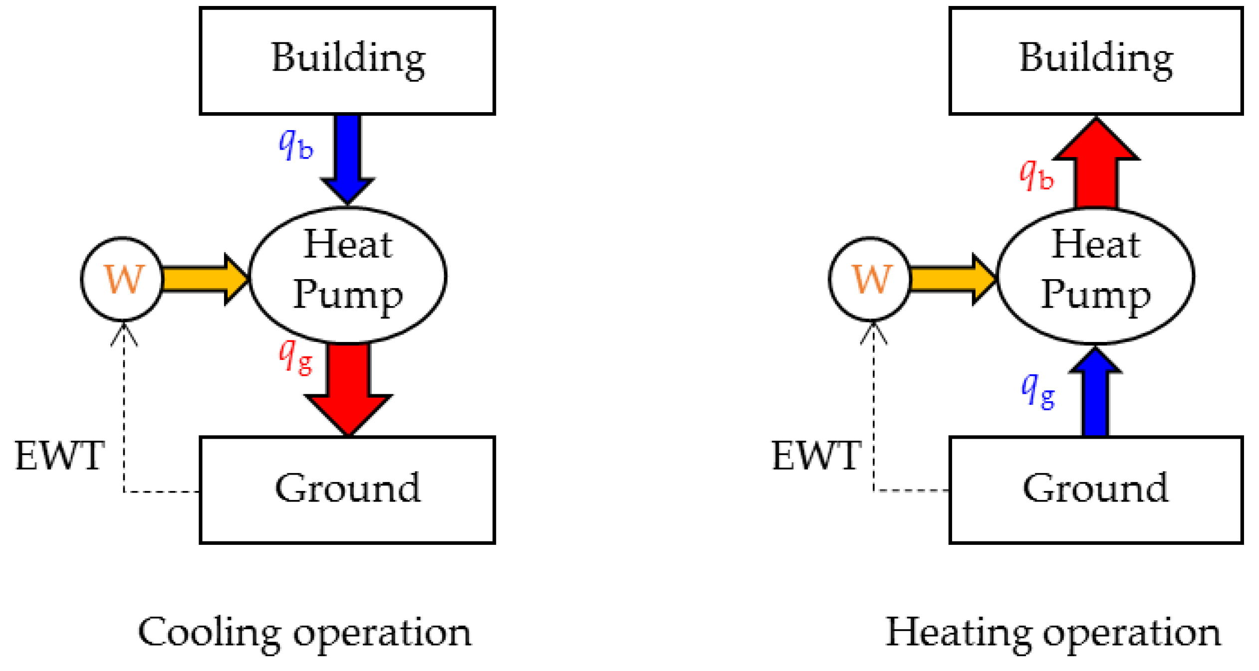
where: μ is 106 when (EWTBHE < EWTset, heating or EWTBHE > EWTset, cooling)
μ is 0 when (EWTset, heating ≤ EWT ≤ EWTset, cooling)
This objective function is very similar to that of Ahmadfard et al. [29]. The objective function in their work was set to minimize the total length of the BHEs. Decreasing the total length of the BHEs results in higher EWTs; thus, this objective function is technically identical to the proposed optimization function of Equation (6).
In the present study, the borehole depth (H) was set to the design variable to be optimized, while the number of BHEs and their arrangement configurations were fixed, and the results were compared with those obtained using the existing GLHE software [4]. The GLHE software includes sizing and hourly simulation of both typical and hybrid GSHP systems, allowing users to define irregular BHE configurations. The other conditions were set to be the same. During the sizing, simulations of 20 years ran iteratively with the DST model to obtain the optimal solution, while the GLHE software used analytical approaches involving aggregated load pulses to accelerate the calculation.
TRNSYS provides an optimization tool (TRNOPT) in the TESS library. TRNOPT is an add-on module that makes TRNSYS compatible with the well-known GenOpt program [31]. GenOpt was developed to solve optimization problems, but only one objective function is specified. In this study, the coordinate search algorithm was used, which is a generalized pattern search algorithm that is effective for local optimization and unconstrained continuous-variable problems.

4. Test Cases

The modification methods presented in Section 2.2 were tested for sizing purposes. The rule-of-thumb-based modification, presented in Section 2.2.1 and Equation (3), is called DST.V1, and DST.V2 represents the regression-based modification that was detailed in Section 2.2.2 and Equation (5). The test configurations are presented in Table 4. I-, L-, U-, and Rec-shapes with different numbers of BHEs were tested. The test borefield shapes were divided into Groups A and B, representing single- and double-line arrangements, respectively. The cases in Group A were similar to the cases used for the development of the modification methods, and those in Group B were new but are commonly found in practice.
Before the modification methods were tested, the cylindrical regular BHE configuration, as shown on the left side of Table 4, was tested to check the genuine difference between the GLHE software and the DST model. The GLHE software is based on the finite-line source model, which is a widely used analytical model [23]. Although the DST model employs a numerical approach, it has been used as a reference model for various analytical models [30,32,33]. Discussions regarding which model is better are not presented in this work; rather, the comparison results are used to deduce the baseline difference.
A slightly cooling-dominant building load profile was used for all test cases, as shown in Figure 3. This building is a conventional Korean apartment located in Seoul consisting of 120 households, each of which has of 84 m2 floor area. Building loads are calculated with set point temperatures of 26 and 22 °C for cooling and heating, respectively. The annual heating demand was 91.97 MWh, and the cooling demand was 125.89 MWh. The peak loads were 63.2 and 96.1 kW for heating and cooling, respectively. The duration of the peak loads was 3 h for both heating and cooling. These values were used as inputs to the DST model. Table 5 presents the monthly demands (qh,total, qc,total) and hourly peak loads (qh,peak, qc,peak), which were required to run the GLHE software.
The test BHEs were of the vertical U-tube type, and the flow rate for each BHE was set as 0.2 L/s. The determination of EWTs is also affected by the coefficient of performance (COP) of the heat pump. The COP can be expressed as a function of the EWT, as indicated by Equation (7). The coefficients α, β, and γ are provided by the heat-pump manufacturer. In this study, the user-defined heat-pump performance was employed, and the same coefficients were used for both the proposed design method using the DST model and the design software. The resulting characteristic curve based on Equation (7) is shown in Figure 4. The parameters required for running the simulations are presented in Table 6. Here, the grout heat capacity in the BHE was used only for the GLHE case, as the DST model does not account for borehole thermal capacity effects.
COPc = α1 + β1EWT + γ1EWT2 (Cooling)COPh = α2 + β2EWT + γ2EWT2 (Heating)

5. Sizing Results

As explained previously, the reference DST model combined with the optimization scheme was compared with the existing GLHE software. Figure 5 shows the simulation results obtained after the completion of the sizing process. The GLHE software did not run such a simulation, as shown in the figure, but this was achieved from the sized borefield. As the monthly demand and hourly peak loads were provided to the GLHE software, the simulation results were expressed in monthly pulses with peaks. The EWTset was 30 °C, and the highest EWT was close to this value. In contrast, the DST-model-based simulation results appeared to be expressed in hourly variations. This simulation was iteratively run to match EWTDST and EWTset. This can be regarded as a final simulation after the objective function converges to a minimum. Although the results of the two methods are very similar, the sizing results for the lengths of the BHEs are slightly different. This is explained later in the paper.
The following figures and tables present the sizing results for test cases obtained via procedures similar to those used for the aforementioned basic case. Figure 6 and Figure 7 and Table 7 present the results related to Group A (one-line arrangements), and Figure 8 and Figure 9 and Table 8 present the results related to Group B (double-line arrangements), as indicated by Table 5. When the results marked with points are placed on the dashed diagonal (y = x), the sizing results of the modified DST model are equal to the GLHE results. Detailed values of total length are presented in Appendix A. Table 7 and Table 8 present the errors (Err) in the total length of the BHEs. The root-mean-square errors (RMSEs) were defined by Equation (8).
Err ( % ) = ( L GLHE L DST / L GLHE × 100 RMSE   ( % )   =   i = 1 n { ( L GLHE L DST i ) / L GLHE i } 2 / n   × 100
For the one-line arrangement, Figure 6 shows the sizing results for different borefield configurations and distances of the BHEs. The test distances of the BHEs ranged from 4 to 7 m. Above all, the red line represents the baseline difference observed in the previous referenced test. When the total length of the BHEs increased (reducing the spacing), the difference increased, indicating undersized lengths for the proposed optimization methods. This suggests that denser arrangements with closer spacing lead to larger differences for the optimization-based sizing (baseline) compared with the existing design method.
For most of the irregular arrangements, the results of the modified DST model exhibited larger deviations from the GLHE results. For the same building loads, the test cases resulted in shorter total lengths of the BHEs compared with the baseline case that adopts cylindrical regular arrangements. This is because the thermal-interference effects among the BHEs were smaller for the irregular arrangements. As indicated by Figure 6, the results of DST.V2 exhibited smaller differences among the borefield shapes, and DST.V1 exhibited larger deviations. Figure 7 shows the differences in the total length of the BHEs, which clearly follow the aforementioned pattern. For instance, DST.V2 exhibited similar differences for a given spacing, but this was not observed in the case of DST.V1. Notably, DST.V1 was deduced from a single I-shape case; thus, the differences in the shape were the smallest among other configurations.
Table 7 presents the Err for each case and the RMSE. The error tended to decrease as the borehole spacing increased, and this pattern was identical to that of the baseline case. The sizing results for Group A were acceptable for both DST.V1 and DST.V2; the RMSE was <5% for most of the cases. This corresponds to a sizing difference of approximately one borehole for a case with a total of >25 boreholes. The L- and U-shapes exhibited the largest and smallest errors, respectively. It is difficult to explain this pattern with physical reasons.
For Group B, the cases of DST.V2 exhibited results similar to those for Group A, but the errors were slightly larger. However, on average, DST.V1 exhibited an error increase by a factor of >2 compared with the Group A cases. This is attributed to the fact that the double-line borefield configurations were not used for the development of the modification methods. For instance, the results for the I-shape case for DST.V1 exhibited larger differences than the Group A cases, with an increase from 1.5% to 12.4% in the RMSE. For several cases, the RMSE for DST.V1 was >10%, corresponding to a sizing difference of >2 boreholes for these examples.
The DST.V2 method was based on the total distance of the BHEs, and theoretically, the model is less sensitive to the borehole shape. Thus, the increased errors may have been due to the baseline differences. Compared with the Group A cases, all the points of DST.V2 for Group B were shifted to the right, where the baseline differences were higher. The DST.V2 results are presented in Figure 10. The points are fairly well aligned near the baseline. The RMSEs based on the GLHE were 3.7% and 5.6% for Groups A and B, respectively. These RMSEs were unchanged when they were evaluated according to the baseline showing 3.7% and 3.6% for Groups A and B, respectively.

6. Conclusions

As the modern GSHP systems becomes complex and diverse, novel sizing tools are required that can size both BHEs and other connected systems simultaneously and perform various engineering analyses. An optimization-based sizing tool using the existing BHE models may satisfy these requirements. DST-model-based sizing methods have been developed using various optimization schemes. The DST model has the advantage of accelerating the calculation by simplifying the BHE arrangement, but this limits the use of the DST model in practical applications, where irregular BHE arrangements are commonly found. Recent developments in modification methods for the DST model allow the model to be utilized for irregular borefields. In this study, the applicability of modified DST models for sizing BHEs placed in irregular ways was investigated. The proposed method combining an optimization scheme and selected modified DST models was tested for sizing purposes, and results were compared with those of the existing GLHE program.
The optimization-based sizing method deviated from the commercial sizing tool. This may have been due to the different BHE models used. The differences increased with the thermal-interference effects in the case of a short spacing of the BHEs. In the test cases of irregular BHEs arrangements, regarding previously developed modification methods, both the rule-of-thumb and regression-based methods exhibited acceptable sizing results, with errors of <5% for one-line arrangements of BHEs. However, the rule-of-thumb method exhibited larger errors (>10%) for double-line arrangements, which were not used in the development of the method. The regression-based method also exhibited slightly larger errors compared with the GLHE results for double-line cases, while the level of the errors was kept unchanged compared with the baseline difference defined by the case of the unmodified DST model. This indicates the effectiveness of the modification method.
To the knowledge of the authors, this study is the first attempt to use the DST model for sizing BHEs placed in irregular borefield configurations. In future studies, various load types and additional arrangements should be examined, and various design alternatives considering entropy or exergy are to be investigated using the proposed method.

Author Contributions

Both authors contributed to performing the simulation tests, developing sizing methods via optimization, and analyzing the results. S.-H.P. drafted the manuscript, and E.-J.K. revised it. Both authors approved the current manuscript.

Funding

This research received no external funding.

Acknowledgments

This work was supported by the Korea Institute of Energy Technology Evaluation and Planning (KETEP) and the Ministry of Trade, Industry & Energy (MOTIE) of the Republic of Korea (No. 2019271010015D). In addition, this work was supported by a National Research Foundation of Korea (NRF) grant funded by the Korean government (MSIP) (No. 2016R1C1B2011097).

Conflicts of Interest

The authors declare no conflict of interest.

Nomenclature

BBorehole spacing (°C)
bCorrelation coefficient (-)
B´Equivalent or modified borehole spacing (°C)
CVolumetric heat capacity (kJ/m3·K)
COPCoefficient of performance (-)
EWTEntering water temperature (°C)
fObjective function
HBorehole depth (m)
NNumber of boreholes (-)
NNumber of data (-)
qHeat transfer rate (W)
sNumber of I-shaped borefields (-)
SSum of borehole spacings (m)
tTime (sec)
TTemperature (°C)
VHeat storage volume (m3)
WWork (W)
XCorrelation factor (-)
Subscript
bBuilding
BHEBorehole heat exchanger
cCooling
DSTDST model
DST.modif.V1DST model with rule-of-thumbs modification
DST.modif.V2DST model with regression based modification
gGround
GLHEGLHE software
hHeating
II-shape borefiled
LL-shape borefiled
RECHollowed rectangular borefiled
setSet point
sfSteady-flux problem in the DST
Local to global heat transfer in the DST
testTest borefield configuration
UU-shape borefiled
Greek
αConstant for COP
βLinear coefficient for COP
γQuadratic coefficient for COP
μPenalty term

Appendix A. Detailed BHE Sizing Results for the Modified DST Models (DST.V1, DST.V2) and the GLHE Software

Table A1. Sizing comparison between the modified DST model and GLHE software: Group A.
BHE SpacingGroup A (1-Line Arrangements)
I-Shape (N = 25)L-Shape (N = 29)U-Shape (N = 26)Hollow-Rectangular (N = 30)
Sustainability 11 04338 i011
25 × 1
Sustainability 11 04338 i012
14,1,14
Sustainability 11 04338 i013
8,1,8,1,8
Sustainability 11 04338 i014
6,1,7,1,6,1,7,1
B(m)GLHE
L (H)
(m)
DST.V1
L (H)
(m)
Err
(m)
DST.V2
L (H)
(m)
Err
(m)
GLHE
L (H)
(m)
DST.V1
L (H)
(m)
Err
(m)
DST.V2
L (H)
(m)
Err
(m)
GLHE
L (H)
(m)
DST.V1
L (H)
(m)
Err
(m)
DST.V2
L (H)
(m)
Err
(m)
GLHE
L (H)
(m)
DST.V1
L (H)
(m)
Err
(m)
DST.V2
L (H)
(m)
Err
(m)
41954
(78.2)
1990
(79.6)
–35.51851
(74.0)
103.12001
(69.0)
1849
(63.8)
152.01885
(65.0)
116.32004
(77.1)
1911
(73.5)
92.81911
(73.5)
92.62096
(69.9)
1979
(65.2)
139.22096
(66.0)
116.7
51862
(74.5)
1897
(75.9)
–35.51798
(71.9)
64.21907
(65.8)
1781
(61.4)
126.21827
(63.0)
79.81897
(73)
1835
(70.6)
62.71840
(70.8)
57.21967
(65.6)
1901
(62.4)
94.21967
(63.4)
66.6
61812
(72.5)
1836
(73.5)
–24.01766
(70.6)
46.71847
(63.7)
1732
(59.7)
115.11788
(61.6)
59.51840
(70.8)
1778
(68.4)
61.91799
(69.2)
40.81886
(62.9)
1841
(60.3)
77.11886
(61.4)
44.4
71780
(71.2)
1790
(71.6)
–10.51730
(69.2)
49.81808
(62.4)
1699
(58.6)
109.01755
(60.5)
53.91798
(69.1)
1737
(66.8)
60.81764
(67.9)
33.51838
(61.3)
1806
(58.9)
71.41838
(60.2)
31.5
Table A2. Sizing comparison between the modified DST model and the GLHE software: Group B.
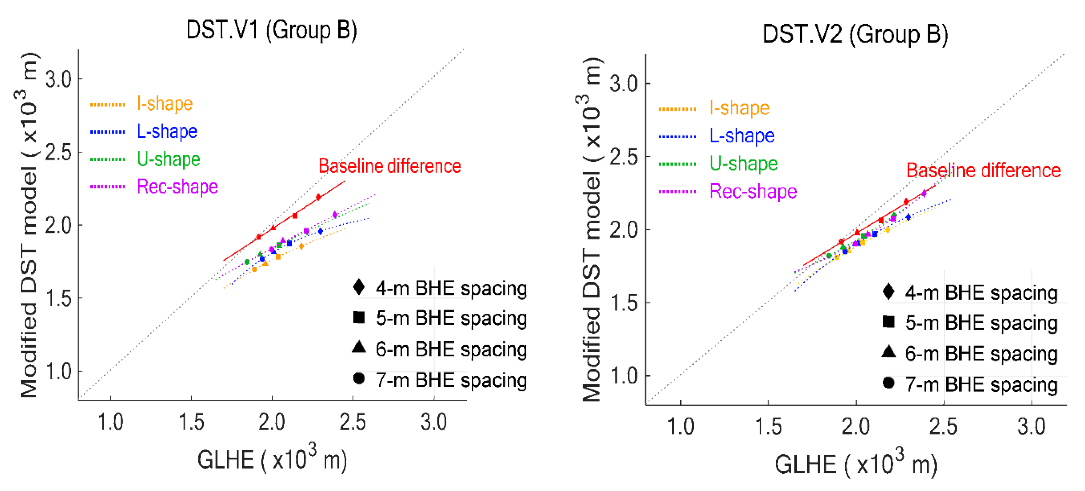
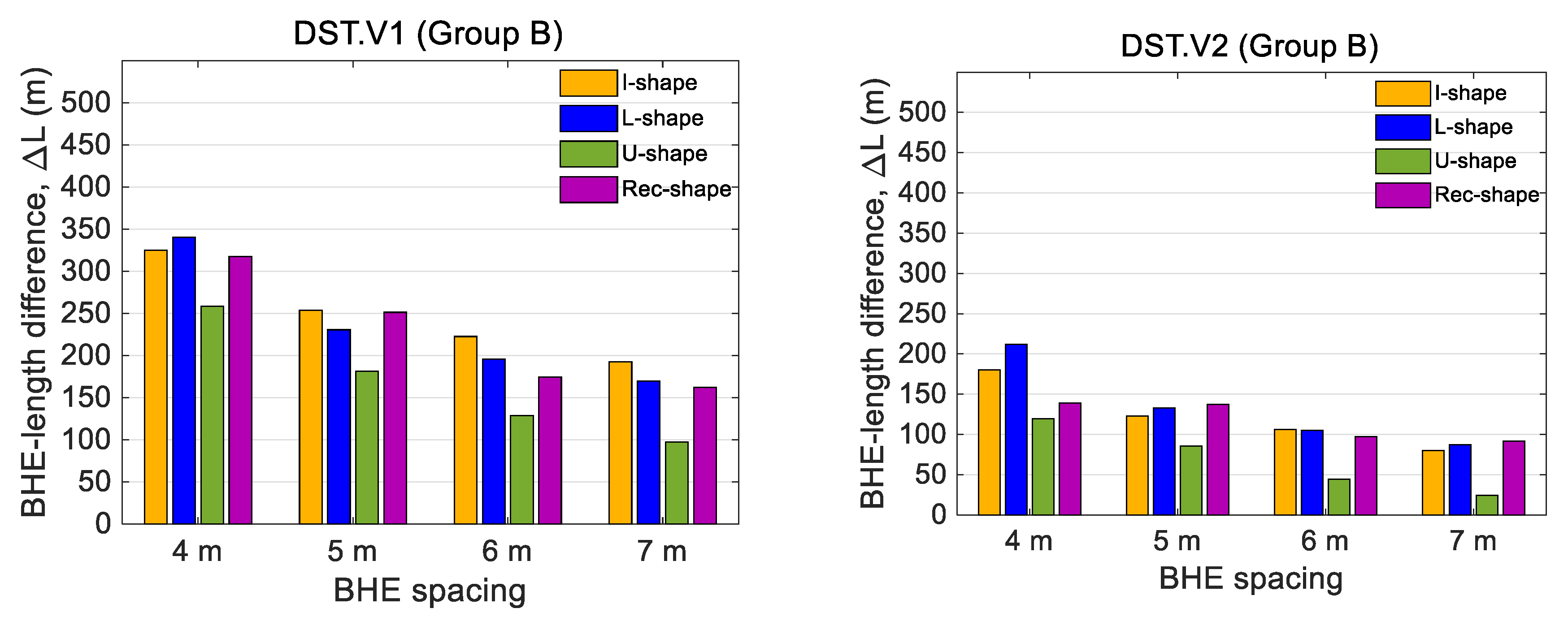
Group B (2-Line Arrangements)
I-Shape (N = 24)L-Shape (N = 28)U-Shape (N = 30)Hollow-Rectangular (N = 28)
Sustainability 11 04338 i015
12 × 2
Sustainability 11 04338 i016
6 × 2, 2 × 2, 6 × 2
Sustainability 11 04338 i017
4 × 2, 2 × 2, 3 × 2, 2 × 2, 4 × 2
Sustainability 11 04338 i018
As shown above
B (m)GLHE
L (H)
(m)
DST.V1
L (H)
(m)
Err
(m)
DST.V2
L (H)
(m)
Err
(m)
GLHE
L (H)
(m)
DST.V1
L (H)
(m)
Err
(m)
DST.V2
L (H)
(m)
Err
(m)
GLHE
L (H)
(m)
DST.V1
L (H)
(m)
Err
(m)
DST.V2
L (H)
(m)
Err
(m)
GLHE
L (H)
(m)
DST.V1
L (H)
(m)
Err
(m)
DST.V2
L (H)
(m)
Err
(m)
42180
(90.8)
1855
(77.3)
325.02000
(83.3)
180.52298
(82.1)
1957
(69.9)
340.52086
(74.5)
211.72215
(76.4)
1956
(67.5)
258.72095
(72.3)
119.52388
(85.3)
2070
(73.9)
317.52249
(80.3)
138.9
52037
(84.9)
1783
(74.3)
253.71914
(79.8)
122.92105
(75.2)
1874
(66.9)
230.71972
(70.4)
133.02043
(70.5)
1862
(64.2)
181.31958
(67.5)
85.62211
(79.0)
1960
(70.0)
251.42074
(74.1)
137.5
61958
(81.6)
1735
(72.3)
222.71852
(77.2)
106.12009
(71.8)
1813
(64.8)
195.71904
(68.0)
105.01925
(66.4)
1797
(62.0)
128.81881
(64.9)
44.72066
(73.8)
1892
(67.6)
174.41969
(70.3)
97.4
71890
(78.7)
1697
(70.7)
192.71810
(75.4)
79.91938
(69.2)
1768
(63.2)
169.71851
(66.1)
87.11845
(63.6)
1747
(60.3)
97.41820
(62.8)
24.41996
(71.3)
1833
(65.5)
162.11904
(68.0)
91.6

References

  1. Sanner, B.; Karytsas, C.; Mendrinos, D.; Rybach, L. Current status of ground source heat pumps and underground thermal energy storage in Europe. Geothermics 2003, 32, 579–588. [Google Scholar] [CrossRef]
  2. Angelino, L.; Dumas, P.; Gindre, C.; Latham, A. EGEC Market Report 2015; European Geothermal Energy Council: Brussels, Belgium, 2016. [Google Scholar]
  3. Gaia Geothermal. Ground Loop Design Premier 2016 Edition User’s Manual. 2016. Available online: https://www.groundloopdesign.com/downloads/GLD_2016/GLD2016_Manual.pdf (accessed on 10 August 2019).
  4. Spitler, J.D. GLHEPRO—A design tool for commercial building ground loop heat exchangers. In Proceedings of the Fourth International Heat Pumps in Cold Climates Conference, Aylmer, QC, Canada, 17–18 August 2000. [Google Scholar]
  5. Blomberg, T.; Claesson, J.; Eskilson, P.; Hellström, G.; Sanner, B. EED v3. 2—Earth Energy Designer; Lund University: Lund, Sweden, 2015. [Google Scholar]
  6. Hackel, S.; Pertzborn, A. Effective design and operation of hybrid ground-source heat pumps: Three case studies. Energy Build. 2011, 43, 3497–3504. [Google Scholar] [CrossRef]
  7. Hénault, B.; Pasquier, P.; Kummert, M. Financial optimization and design of hybrid ground-coupled heat pump systems. Appl. Eng. 2016, 93, 72–82. [Google Scholar] [CrossRef]
  8. Ciani Bassetti, M.; Consoli, D.; Manente, G.; Lazzaretto, A. Design and off-design models of a hybrid geothermal-solar power plant enhanced by a thermal storage. Renew. Energy 2018, 128, 460–472. [Google Scholar] [CrossRef]
  9. Park, H.; Lee, J.S.; Kim, W.; Kim, Y. Performance optimization of a hybrid ground source heat pump with the parallel configuration of a ground heat exchanger and a supplemental heat rejecter in the cooling mode. Int. J. Refrig. 2012, 35, 1537–1546. [Google Scholar] [CrossRef]
  10. Salvalai, G. Implementation and validation of simplified heat pump model in IDA-ICE energy simulation environment. Energy Build. 2012, 49, 132–141. [Google Scholar] [CrossRef]
  11. Klein, S.A.; Beckman, W.A.; Mitchell, J.W.; Duffie, J.A.; Duffie, N.A.; Freeman, T.L.; Mitchell, J.C. Trnsys 17: A Transient System Simulation Program; Solar Energy Laboratory, University of Wisconsin: Madison, WI, USA, 2010. [Google Scholar]
  12. Hellström, G. Duct Ground Heat Storage Model Manual for Computer Code; Department of Mathematical Physics, University of Lund: Lund, Sweden, 1989. [Google Scholar]
  13. Bayer, P.; de Paly, M.; Beck, M. Strategic optimization of borehole heat exchanger field for seasonal geothermal heating and cooling. Appl. Energy 2014, 136, 445–453. [Google Scholar] [CrossRef]
  14. Huang, S.; Ma, Z.; Wang, F. A multi-objective design optimization strategy for vertical ground heat exchangers. Energy Build. 2015, 87, 233–242. [Google Scholar] [CrossRef] [Green Version]
  15. Zhang, C.; Hu, S.; Liu, Y.; Wang, Q. Optimal design of borehole heat exchangers based on hourly load simulation. Energy 2016, 116, 1180–1190. [Google Scholar] [CrossRef]
  16. Pu, L.; Qi, D.; Xu, L.; Li, Y. Optimization on the performance of ground heat exchangers for GSHP using Kriging model based on MOGA. Appl. Eng. 2017, 118, 480–489. [Google Scholar] [CrossRef]
  17. Xia, L.; Ma, Z.; Kokogiannakis, G.; Wang, S.; Gong, X. A model-based optimal control strategy for ground source heat pump systems with integrated solar photovoltaic thermal collectors. Appl. Energy 2018, 228, 1399–1412. [Google Scholar] [CrossRef] [Green Version]
  18. Bertagnolio, S.; Bernier, M.; Kummert, M. Comparing vertical ground heat exchanger models. J. Build. Perform. Simul. 2012, 5, 369–383. [Google Scholar] [CrossRef]
  19. Park, S.H.; Kim, J.Y.; Jang, Y.S.; Kim, E.J. Development of a multi-objective sizing method for borehole heat exchangers during the early design phase. Sustainability 2017, 9, 1876. [Google Scholar] [CrossRef]
  20. Park, S.H.; Jang, Y.S.; Kim, E.J. Using duct storage (DST) model for irregular arrangements of borehole heat exchangers. Energy 2018, 142, 851–861. [Google Scholar] [CrossRef]
  21. Pahud, D.; Fromentin, A.; Hadorn, J.C. The Duct Ground Heat Storage Model (DST) for TRNSYS Used for the Simulation of Heat Exchanger Piles, User Manual; École Polytech & Fédérale Lausanne: Paris, France; Lausanne, Switzerland, 1996. [Google Scholar]
  22. Chapuis, S.; Bernier, M. Seasonal storage of solar energy in borehole heat exchangers. In Proceedings of the 11th International IBPSA Conference, Glasgow, Scotland, 27–30 July 2009. [Google Scholar]
  23. Kim, E.J. TRNSYS g-function generator using a simple boundary condition. Energy Build. 2018, 172, 192–200. [Google Scholar] [CrossRef]
  24. Rad, F.M.; Fung, A.S.; Rosen, M.A. An integrated model for designing a solar community heating system with borehole thermal storage. Energy Sustain. Dev. 2017, 36, 6–15. [Google Scholar] [CrossRef]
  25. Malmberg, M.; Lindståhl, H. High temperature borehole thermal energy storage—A case study. In Proceedings of the IGSHPA Research Track, Stockholm, Sweden, 18–20 September 2018. [Google Scholar] [CrossRef]
  26. Panno, D.; Buscemi, A.; Beccali, M.; Chiaruzzi, C.; Cipriani, G.; Ciulla, G.; Di Dio, V.; Lo Brano, V.; Bonomolo, M. A solar assisted seasonal borehole thermal energy system for a non-residential building in the Mediterranean area. Sol. Energy 2018, 1–13. [Google Scholar] [CrossRef]
  27. Hackel, S.; Nellis, G.; Klein, S. Optimization of hybrid geothermal heat pump systems. In Proceedings of the 9th International IEA Heat Pump Conference, Zürich, Switzerland, 20–22 May 2008. [Google Scholar]
  28. Eskilson, P. Thermal Analysis of Heat Extraction Boreholes. Ph.D. Thesis, Department of Mathematical Physics, University Lund, Lund, Sweden, 1987. [Google Scholar]
  29. Park, S.H.; Jeon, B.K.; Jang, Y.S.; Kim, E.J. Multi-objective Sizing Optimization of Borehole Heat Exchangers. In Proceedings of the 15th IBPSA Conference, San Francisco, CA, USA, 7–9 August 2017. [Google Scholar]
  30. Kim, E.J.; Bernier, M.; Cauret, O.; Roux, J.J. A hybrid reduced model for borehole heat exchangers over different time-scales and regions. Energy 2014, 77, 318–326. [Google Scholar] [CrossRef]
  31. Wetter, M. GenOpt-A generic optimization program. In Proceedings of the 7th International IBPSA Conference, Rio de Janeiro, Brazil, 13–15 August 2001. [Google Scholar]
  32. Spitler, J.D.; Cullin, J.; Bernier, M.; Kummert, M.; Cui, P.; Liu, X.; Fisher, D. Preliminary intermodel comparison of ground heat exchanger simulation models. In Proceedings of the 11th International Thermal Energy Storage Conference, Stockholm, Sweden, 14–17 June 2009. [Google Scholar]
  33. Zhang, X.; Zhang, T.; Jiang, Y.; Li, B. Improvement on an analytical finite line source model considering complex initial and boundary conditions: Part 1, model development and validation. Energy Build. 2019, 198, 1–10. [Google Scholar] [CrossRef]
Figure 1. Schematic of the 19-borehole configuration in the storage volume of the DST model.
Sustainability 11 04338 g001
Figure 2. Schematic of the energy conservation in GSHP systems.
Sustainability 11 04338 g002
Figure 3. Hourly building loads over a year.
Sustainability 11 04338 g003
Figure 4. Heat-pump characteristic curves for the EWT and COP.
Sustainability 11 04338 g004
Figure 5. Simulation results for the EWTs (A: GLHE; B: DST and TRNOPT).
Sustainability 11 04338 g005aSustainability 11 04338 g005b
Figure 6. Comparison of the BHE sizing results between the GLHE software and the modified DST models for Group A.
Sustainability 11 04338 g006
Figure 7. Differences in the BHE total length between the modified DST models and the GLHE software for Group A.
Sustainability 11 04338 g007
Figure 8. Comparison of the BHE sizing results between the GLHE software and the modified DST models for Group B.
Sustainability 11 04338 g008
Figure 9. Differences in the BHE total length between the modified DST models and the GLHE software for Group B.
Sustainability 11 04338 g009
Figure 10. Sizing results of DST.V2 for Groups A and B.
Sustainability 11 04338 g010
Table 1. Literature review for GHE sizing optimization using TRNSYS and DST.
AuthorsGHE ModelsDesign VariablesObjective Functions
S. Hackel et al. [6]DST model
  • Length of BHE
  • Cooling tower capacity
  • Tset for control
  • min (life-cycle-cost)
S. Huang et al. [14]DST model
  • Borefields
  • GHE materials
  • Flow rate
  • min (total cost)
  • max (energy)
C. Zhang et al. [15]DST model
  • Borehole depths
  • Borehole spacings
  • Number of boreholes
  • min (EWTBHE-EWTset)
L. Pu et al. [16]DST model
  • U-tube spacing
  • U-tube diameter
  • Reynolds number
  • EWT
  • min ( Δ entropy)
  • max (efficiency)
L. Xia et al. [17]DST model
  • Pump frequency
  • Leaving load side temp
  • Leaving source side temp
  • min (energy)
  • max (COP)
Table 2. Test borehole configurations and equivalent spacing in the modified DST model [20].
BHE ConfigurationCylindricalRec-ShapeU-ShapeL-ShapeI-Shape
Tested irregular BHEs configurations Sustainability 11 04338 i001 Sustainability 11 04338 i002 Sustainability 11 04338 i003 Sustainability 11 04338 i004 Sustainability 11 04338 i005
Borehole spacingB
Equivalent configurations for the DST model
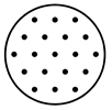
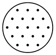
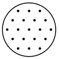
 Sustainability 11 04338 i001 Sustainability 11 04338 i006 Sustainability 11 04338 i007 Sustainability 11 04338 i008 Sustainability 11 04338 i009
Equivalent borehole spacing B = B´<B´REC<B´U<B´L<B´I
Table 3. Correlation coefficients of Equation (4) [20].
ibiXi
0−6.7140701Constant
11.6921897B
2−0.0442890B2
34.6624113Stest/SDST
4−0.6152736(Stest/SDST)2
50.1001986B × (Stest/SDST)
Table 4. Test configurations for BHE-sizing comparisons with modified DST models.
AxisymmetricGroup A (1-Line Arrangements)
CylindricalI-shapeL-shapeU-shapeRec-shape
(N = 19)(N = 25)(N = 29)(N = 26)(N = 30)
Sustainability 11 04338 i010
Reference
DST model
Sustainability 11 04338 i011 Sustainability 11 04338 i012 Sustainability 11 04338 i013 Sustainability 11 04338 i014
25 × 114,1,148,1,8,1,86,1,7,1,6,1,7,1
Group B (2-line arrangements)
I-shapeL-shapeU-shapeRec-shape
(N = 24)(N = 28)(N = 30)(N = 28)
Sustainability 11 04338 i015 Sustainability 11 04338 i016 Sustainability 11 04338 i017 Sustainability 11 04338 i018
12 × 26 × 2, 2 × 2, 6 × 24 × 2, 2 × 2, 3 × 2, 2 × 2,4 × 2As shown above
Table 5. Monthly building demands for heating and cooling.
LoadsJanuaryFebruaryMarchAprilMayJuneJuleAugustSeptemberOctoberNovemberDeccenber
qh,total (MWh)24.719.211.22.3000000.911.921.9
qc,total (MWh)0003.915.424.928.128.718.07.100
qh,peak (kW)63.253.641.125.90000013.643.555.1
qc,peak (kW)00039.379.988.896.192.676.242.800
Table 6. Parameters used for TRNSYS and the GLHE software.
ParameterValueUnit
Borehole
Header depth1M
Borehole radius55Mm
U-tube spacing20.1Mm
U-tube inside diameter13Mm
U-tube outside diameter16Mm
Flow rate per borehole0.2L/s
Borehole thermal resistance0.1395K/(W·m)
Grout heat capacity3900kJ/(m3·K)
Grout thermal conductivity2W/(m·K)
Pipe heat capacity1542kJ/(m3·K)
Pipe thermal conductivity2W/(m·K)
Ground
Thermal conductivity2W/(m·K)
Heat capacity2160.5kJ/(m3·K)
Initial temperature10°C
Far-field temperature10°C
Fluid
Density1022kg/m3
Specific heat3960kJ/(m3·K)
Thermal conductivity0.44W/(m·K)
Table 7. Differences in the sizing results between the GLHE software and the modified DST model (Group A: 1-line array).
BHIE Spacing (m)Base-Line
Diff
(%)
DST.V1DST.V2
ErrorRMSE
(%)
ErrorRMSE
(%)
I
(%)
L
(%)
U
(%)
Rec
(%)
I
(%)
L
(%)
U
(%)
Rec
(%)
44.1−1.87.64.66.65.65.35.84.65.65.3
53.7−1.96.63.34.84.53.54.23.03.43.5
61.3−1.36.23.44.14.12.63.22.22.42.6
70.1−0.66.03.43.94.02.83.01.91.72.4
RMSE
(%)
3.01.56.63.75.04.63.74.23.13.63.7
Table 8. Differences in the sizing results between the GLHE software and the modified DST model (Group B: 2-line array).
BHIE Spacing (m)Base-Line
Diff.
(%)
DST.V1DST.V2
ErrorRMSE
(%)
ErrorRMSE
(%)
I
(%)
L
(%)
U
(%)
Rec
(%)
I
(%)
L
(%)
U
(%)
Rec
(%)
44.114.914.811.713.313.78.39.25.45.87.4
53.712.511.08.911.411.06.06.34.26.25.8
61.311.49.76.78.49.25.45.22.34.74.6
70.110.28.85.38.18.34.24.51.34.63.9
RMSE
(%)
3.012.411.38.510.510.86.26.63.75.45.6

