Abstract
Internet of Vehicles (IoV), which enables information exchange among vehicles, infrastructures and environment, is considered to have great potential for improving traffic. However, information delays may lead to driver’s incorrect operations and have a negative impact on traffic flow. To improve traffic safety and reduce energy dissipation under IoV conditions, this paper intends to explore a more favorable driving strategy, which may weaken the adverse effects of information delays. This study regarding driving strategy is based on an improved car-following model with consideration of Global Optimality (GO-FVD model). Linear stability analysis and numerical simulations are carried out to explore the effects of Global Optimality on traffic flow. Results confirm that Global Optimality contributes to enhancing the stability and safety of traffic flow as well as depressing the energy dissipation. In particular, it is more suitable for the low-density traffic to account for Global Optimality. These results can provide theoretical support for the development of favorable driving strategy under IoV conditions, which will promote the sustainable development of intelligent transportation.
1. Introduction
Traffic problems such as traffic accidents, congestion, and energy consumption have aroused wide concern in modern society [1,2,3,4,5,6,7]. Intelligent Transportation System (ITS) is considered to have great potential for solving these problems [8,9,10,11,12,13,14]. As an integral component of future ITS, Internet of Vehicles (IoV) enables the information exchange among vehicles, infrastructures and environment [15,16,17]. Accordingly, drivers will be provided with more traffic information, which supports their driving tasks. For instance, the driving states of vehicles in the vicinity can be obtained, according to which drivers adjust their own driving states. However, the states of vehicles are constantly changing, and transfer delays of information are common [18,19]. As a result, drivers may receive untimely information, leading to their incorrect operations which have negative influences on traffic. How to weaken the adverse effects of transfer delays and improve traffic under IoV conditions? Besides the advances in information transmission technology, the improvement of driving strategy is of great importance as well. However, the question has not been extensively investigated from the perspective of driving strategy.
To this end, the purpose of this paper is to explore a driving strategy that is able to improve traffic safety and reduce energy dissipation under IoV conditions. Specifically, the strategy with consideration of Global Optimality is the main focus of this study. Here, Global Optimality means that the average headway of traffic flow on a road with a certain length is taken into account when drivers adjust their driving states. This is because the average headway reflects the overall traffic situation on a road segment [20]. Furthermore, it is relatively stable information and little influenced by transfer delays. Consequently, this paper proposes the hypothesis that the traffic will be improved by considering Global Optimality under IoV conditions.
In addition, microscopic traffic models are not only important approaches to study traffic problems but also beneficial evaluation tools for ITS [21]. Particularly, car-following models can effectively describe interactions of vehicles and capture complex characteristics of vehicle dynamics in real traffic [22]. Traffic problems in ITS environment have been widely studied using car-following models as shown in the literature review part. Nonetheless, most of these models just considered the effects of vehicles in the vicinity on drivers, but the Global Optimality was neglected. Thus, there is a need for an improved car-following model to explore the effects of Global Optimality on traffic under IoV conditions.
Therefore, to investigate the hypothesis proposed above, this paper formulates an improved car-following model with consideration of Global Optimality (GO-FVD model). Based on GO-FVD model, the effects of Global Optimality on traffic stability, safety as well as energy dissipation are tested by analytical and numerical methods. The new model will provide theoretical reference for further study with respect to traffic problems in IoV environment. The findings in this study may help to improve the traffic under IoV conditions, which will promote the sustainable development of intelligent transportation.
2. Literature Review
Car-following models describe the vehicle-by-vehicle following process in traffic flow. The earliest framework of car-following model was developed by Pipes [23] and Reuschel [24]. The idea of this framework is that the motion of the following vehicle is affected by the stimulus from the preceding vehicle. Since then, numerous classical car-following models have been put forward consecutively [21,25,26,27,28,29,30,31,32,33,34]. In general, these classical models can be categorized into six types, including stimulus–response [25,26], safety distance [27,28], desired measures [29,30], optimal velocity [21,31,32], psycho-physical [33] and artificial intelligence [34] models. Among them, there are some models that have especially received considerable attention. For example, Newell model [26], optimal velocity (OV) model [31], full velocity difference (FVD) model [21] and intelligent driver (ID) model [30]. These models replicate traffic phenomenon by mathematical equations, and thus help to better understand traffic dynamics.
Newell model [26] holds that each vehicle has its optimal velocity. Assuming the position of vehicle n at time t is , then the optimal velocity of vehicle n at time t can be represented by , which depends on the headway between vehicle n and the preceding vehicle n + 1, and . The velocity of vehicle n will be adjusted to its optimal velocity within a time lag τ. This time lag is caused by driver’s reaction delay and vehicle’s response delay. Mathematically, Newell model can be defined as:
where is the velocity of vehicle n at time .
The unrealistically high acceleration was observed in Newell model when the traffic light changes from red to green. To address this issue, Bando et al. proposed OV model [31], which is described as:
where α is drivers’ sensitivity that can be regarded as the reciprocal of drivers’ reaction time. refers to the acceleration of vehicle n at time t. Since OV model adopts acceleration equation instead of velocity equation to replicate traffic phenomenon, it can describe more properties of the real traffic flow.
However, comparison with the field data shows that OV model still produces too high acceleration and unrealistic deceleration. To overcome the shortages, Helbing and Tilch proposed the generalized force (GF) model which took into account the negative velocity difference between the current vehicle and the preceding vehicle [32]. Based on OV model and GF model, Jiang et al. proposed FVD model with consideration of both negative and positive velocity differences [21]. The dynamic equation is formulated as:
where refers to the velocity difference between vehicle n + 1 and vehicle n, and β is the coefficient parameter. Obviously, traffic dynamics can be better described by FVD model.
ID model was proposed by Treiber et al. in 2000 [30]. The main idea of ID model is that drivers expect to maintain a constant distance from the preceding vehicle. However, drivers’ reaction time (or sensitivity) is ignored in this model. Thus, ID model may be more suitable for autonomous vehicles.
Recent technology advances have significantly pushed forward the development of ITS. The realistic influences and development prospects of ITS have been studied extensively [8,9,10,11,12,13,14,15,16,35,36,37]. Specifically, the adaptive cruise control (ACC) strategy and the Vehicle to Vehicle (V2V) communication have attracted considerable attention. Great efforts have been devoted to study the effects of these new environments on traffic based on car-following models.
ACC vehicles, based on a control algorithm, automatically adjust the velocity to maintain their proper headway from the vehicle in front. The constant safe time headway is an important quantity in this control algorithm [38]. ID model introduces the parameter denoting the time headway and appears to be a good basis for the ACC system. To this end, ID model was widely extended with consideration of real traffic factors under the condition of ACC system [39,40,41]. In 2007, Kesting et al. differentiated parameter sets of ID model to simulate human and automated (ACC) driving behaviors. They found that a small proportion of ACC vehicles led to a drastic reduction of traffic congestion [39]. In 2010, Kesting et al. further proposed an enhanced ID model to simulate the influences of different ACC strategies on the maximum traffic capacity. Results suggested that 1% more ACC vehicles would increase the capacities by about 0.3% [40]. To simulate various ACC behaviors for a microscopic traffic simulator, Horiguchi and Oguchi proposed car-following models for three ACC types based on the derivation of ID model (IDM+) [41].
Through wireless communication technology, V2V communication enables vehicles to exchange driving information within a given communication range. Traffic characteristics in V2V environment will therefore be changed as well. Accounting for driver’s timely reaction under the condition of V2V communication, Hua et al. extended the Newell model. Based on this model, they explored the effects of V2V communication on traffic flow during vehicle starting and braking process as well as in the event of an emergency [42]. Additionally, many studies held that, in light of V2V availability, drivers could respond to vehicles in the vicinity [43,44,45]. Wang et al. argued that considering multiple vehicles in front would enhance the stability of traffic flow. Thus, they proposed the Multiple Velocity Difference (MVD) model by introducing multiple velocity differences into the FVD model [43]. In addition to the velocity difference, another Multiple Car-Following (MCF) model took into account the headways of multiple vehicles in front [44]. Sun et al. formulated a car-following model under V2V communication condition based on OV model and investigated the effects of feedback control signal on traffic flow [45]. Results of these studies were consistent, which indicated that considering information of multiple vehicles in front contributed to suppressing traffic congestion as well as depressing energy consumption.
Notably, it is pointed out that transfer delays of information are common, which has negative effects on traffic [18,19]. However, there are few studies with respect to driving strategies that will weaken these adverse effects. Therefore, it is of great importance to explore such driving strategy. This paper holds that the consideration of Global Optimality appears to be a favorable strategy in IoV environment. In addition, previous studies have verified that car-following models are helpful tools for predicting the effects of ACC systems and V2V communication on traffic. IoV is an integral component of future ITS and the extension of V2V communication. Therefore, this paper will investigate the effects of Global Optimality on traffic based on an improved car-following model under IoV conditions.
3. Methodology
As described above, FVD model is especially suitable for the study of traffic phenomenon under IoV conditions. Therefore, to explore the effects of Global Optimality on traffic, GO-FVD model is first formulated in this study. Based on GO-FVD model, linear stability analysis is then conducted to deduce the stability condition of traffic flow. Finally, numerical simulations are carried out to investigate the specific effects of Global Optimality on traffic stability, traffic safety and energy consumption.
3.1. Model
In the environment of IoV, as mentioned in the introduction part, Global Optimality can be reflected by the average headway that is relatively stable information. Consequently, in addition to considering the preceding vehicle, taking the average headway into account may help suppress driver’s incorrect operations. According to this standpoint, this paper, based on FVD model, proposes a car-following model with consideration of Global Optimality (GO-FVD model). The new model can be described as:
where L is the global length of a road and N is the global number of vehicles (Figure 1). denotes the ideal velocity, which is the function of the average headway and refers to the desired velocity for the uniform flow. is the optimal velocity, which depends on the headway of vehicle n and represents the desired velocity of the current vehicle. The Global Optimality can be achieved only when the velocities of all vehicles are equal to the ideal velocity. Parameter λ is the coefficient of velocity difference between the ideal velocity and the current velocity. Parameter γ is the coefficient of velocity difference between the ideal velocity and the optimal velocity. Other variables have the same meanings as that in Equations (1) to (3).
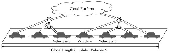
Figure 1.
Car following under the condition of Internet of Vehicles.
According to the calibration carried out by Helbing and Tilch [32], the optimal velocity () function and the ideal velocity () function in Equation (4) are given by Equations (5) and (6).
where is the vehicle length, and . , , and are parameters, and their estimated values are: , , , .
3.2. Linear Stability Analysis
Stability analysis is to investigate the influence of perturbations on traffic flow. If the traffic is stable, small perturbation will gradually disappear during the propagation process. Conversely, if the traffic is unstable, small perturbation will propagate upstream along the traffic flow, evolving the traffic flow into traffic congestion gradually. The linear stability of GO-FVD model will be explored using the perturbation analysis method [43]. The specific analysis steps are as follows.
Suppose that vehicles move on a road with the uniform headway b and velocity V(b), then the steady state solution is:
where is the initial position of vehicle n at time t. Inserting a small perturbation and Equation (7) into Equation (4), the linearized equation is obtained by using Taylor expansion:
where , . Let , where and are respectively the frequency and wave number. Then is expanded according to the Fourier Series. Substituting it into Equation (8), Equation (9) is given:
Let , which is an imaginary number. Equation (10) is deduced using Euler formula :
Assuming the real part and the imaginary part in Equation (10) are both zero, it yields:
From Equation (12), Equation (13) is obtained:
Substituting Equation (13) into Equation (11) and taking , , then
Further, Equation (15) is deduced from Equation (14):
The neutral stability curve (Equation (16)) is obtained by using L’Hospital’s rule when .
Finally, the linear stability conditions can be obtained.
3.3. Numerical Simulations
Numerical simulations can visually replicate the motion characteristics of traffic flow. Thus, the stability, safety and energy dissipation of traffic flow can be investigated by means of numerical simulations. In this study, numerical simulations are performed under the periodic boundary condition by applying Matlab R2016b. The initial simulation state is that N vehicles are uniformly distributed on the road with global length L [21]. In addition, β = 0.2 and the time interval is [43]. The perturbation added to the above stable flow is . Values of other parameters are the same as that in Equations (5) and (6). The evolution processes as well as the energy dissipation of traffic flow are simulated by varying the values of parameters λ and γ under different sensitivities. In the simulations, the global number of vehicles is N = 100 and the global length of road is L = 1500 m [21]. Here, the energy dissipation refers to the additional consumption of energy caused by the perturbation. Energy dissipation for vehicle n from time t to can be formulated as Equation (17) [46,47].
where m is the vehicle mass, and m = 1500 kg. Then, energy dissipation rate () is given by Equation (18). Besides, total energy dissipation for each vehicle () during time T can be described by Equation (19).
Furthermore, to test the applicability of GO-FVD model under the conditions of different average headways, velocity distributions of all vehicles are simulated by varying the global number of vehicles on a road with the global length L = 6000 m. The simulations are conducted under different parameters λ and γ at low sensitivity α = 1.0.
4. Results and Discussion
4.1. Analytical Results
According to the analytical methods listed in Section 3.2, the linear stability criterion for GO-FVD model is given by
The GO-FVD model presented in Equation (4) reduces to OV model when β = 0, λ = 0, γ = 0. Thus, the stability condition is
When β ≠ 0, λ = 0, γ = 0, the stability condition for FVD model is
To display the linear stability results shown in Equations (20) to (22) more intuitively, Figure 2 plots the neutral stability curves for GO-FVD model, FVD model and OV model. The three curves in Figure 2 denote the neutral stability conditions for these three models respectively. The areas below the neutral stability curves are unstable regions and the areas above the curves represent stable regions. One can observe that, compared with OV model (β = 0, λ = 0, γ = 0) and FVD model (β = 0.2, λ = 0, γ = 0), the stable region of GO-FVD model (β = 0.2, λ = 0.15, γ = 0.1) is significantly enlarged. Analytical results indicate that the stability of traffic flow will be enhanced with consideration of Global Optimality.
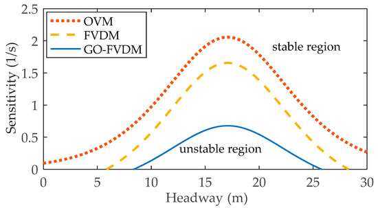
Figure 2.
The neutral stability curves for OV model (β = 0, λ = 0, γ = 0), FVD model (β = 0.2, λ = 0, γ = 0) and GO-FVD model (β = 0.2, λ = 0.15, γ = 0.1).
4.2. Simulation Results
4.2.1. Evolution Processes of Traffic Flow
The evolution processes of traffic flow are simulated to investigate the effects of Global Optimality on traffic stability and safety.
• The headway evolutions at low sensitivity
The headway evolution of traffic flow is an important indicator for traffic stability, which can reflect the development of traffic congestion. Specifically, the greater the headway fluctuation, the more unstable the traffic flow is. Figure 3 exhibits the headway evolutions for FVD model (λ = 0, γ = 0) and GO-FVD model (λ = 0.15, γ = 0.1; λ = 0.2, γ = 0.2) at low sensitivity α = 1.0. Patterns (a–d) in Figure 3 correspond to t = 100 s, t = 200 s, t = 400 s and t = 2000 s after the perturbation, respectively. Figure 3a shows that the headway fluctuates at t = 100 s under different λ and γ due to the small perturbation. Comparing Figure 3a–d, it can be observed that the headway fluctuation for FVD model becomes more and more severe as time goes on, suggesting the traffic congestion may eventually occur. However, as shown in Figure 3c, the headway fluctuation for GO-FVD model (λ = 0.2, γ = 0.2) almost disappears at t = 400 s. Thus, the traffic flow returns to the stable state. Similarly, the traffic flow for GO-FVD model (λ = 0.15, γ = 0.1) will become stable at t = 2000 s as well (Figure 3d). It is demonstrated that GO-FVD model is more conducive to the stability of traffic flow than FVD model. Traffic congestion will be alleviated accordingly. Moreover, the fluctuations are decreased with the increase of parameters λ and γ. Namely, traffic stability will be strengthened with more consideration given to Global Optimality.
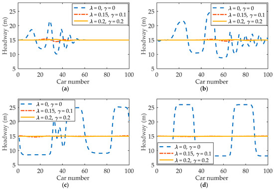
Figure 3.
The headway evolutions for FVD model (λ = 0, γ = 0) and GO-FVD model (λ = 0.15, γ = 0.1; λ = 0.2, γ = 0.2) at low sensitivity α = 1.0: (a) t = 100 s; (b) t = 200 s; (c) t = 400 s and (d) t = 2000 s.
• The acceleration profiles at low sensitivity
The severe acceleration fluctuation means that drivers may brake suddenly or accelerate abruptly. Such behaviors are harmful to traffic safety. Thus, the safety of traffic flow can be explored by analyzing acceleration profiles. Figure 4 displays the acceleration profiles at low sensitivity α = 1.0 under different t for the cases (a) FVD model (λ = 0, γ = 0), (b) GO-FVD model (λ = 0.15, γ = 0.1) and (c) GO-FVD model (λ = 0.2, γ = 0.2). Comparing the three cases in Figure 4, it is clear that at t = 100 s, the amplitude of acceleration for FVD model (Figure 4a) is greater than that for GO-FVD model (Figure 4b,c). Additionally, at t = 2000 s, the acceleration fluctuation is amplified for FVD model (Figure 4a) but is greatly weakened for GO-FVD model (Figure 4b,c). In particular, the accelerations of all vehicles approach to zero in Figure 4c. These simulation results indicate that Global Optimality can reduce driver’s unsafe driving behaviors such as sudden acceleration and deceleration. Furthermore, as parameters λ and γ increase separately, the safety of traffic flow will be improved correspondingly.
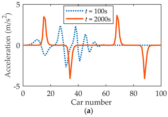

Figure 4.
The acceleration profiles at low sensitivity α = 1.0 under different t: (a) FVD model (λ = 0, γ = 0); (b) GO-FVD model (λ = 0.15, γ = 0.1) and (c) GO-FVD model (λ = 0.2, γ = 0.2).
• The space-time evolutions of velocity at high sensitivity
The velocity fluctuation of traffic flow is also an important factor linked to traffic stability and safety. To further exam the effects of Global Optimality on the safety and stability of traffic flow at high sensitivity, numerical simulations about the velocity evolutions are carried out when α = 2.0. Figure 5 illustrates the space-time evolutions of velocity before t = 400 s under different λ and γ, where (a) FVD model (λ = 0, γ = 0), (b) GO-FVD model (λ = 0.15, γ = 0.1) and (c) GO-FVD model (λ = 0.2, γ = 0.2). It is found that the velocity fluctuations will disappear in course of time for all the three cases. Despite this, traffic flow for FVD model (Figure 5a) evolves to uniform flow slower than that for GO-FVD model (Figure 5b). It is explicit that at high sensitivity, the safety and stability of traffic flow are also enhanced while considering Global Optimality. Moreover, compared with Figure 5b, the velocity fluctuations in Figure 5c are smaller, which means it is more conducive to stable and safe traffic when the values of parameters λ and γ are greater.
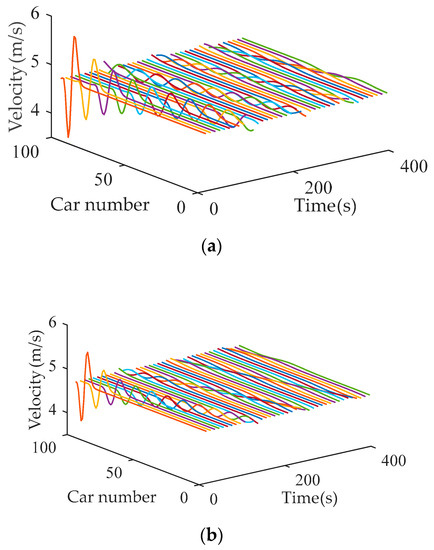
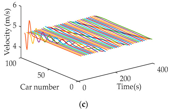
Figure 5.
The space-time evolutions of velocity at α = 2.0 before t = 400s: (a) FVD model (λ = 0, γ = 0); (b) GO-FVD model (λ = 0.15, γ = 0.1) and (c) GO-FVD model (λ = 0.2, γ = 0.2).
From the simulations of the evolution processes of traffic flow, it is illustrated that, under the strategy with consideration of Global Optimality, traffic stability and safety are improved at both low and high sensitivities. Furthermore, the stability and safety are enhanced with the increase of parameters λ and γ.
4.2.2. Energy Dissipation of Traffic Flow
Energy consumption is another traffic problem that has attracted widespread concern. Unstable traffic flow will result in energy dissipation. This section will study the effects of Global Optimality on energy dissipation of traffic flow by conducting numerical simulations.
Figure 6 illustrates the curves for energy dissipation rate under different parameters λ and γ for the cases (a) α = 1.0 and (b) α = 2.0. It is found that at low sensitivity (Figure 6a), of traffic flow for FVD model (λ = 0, γ = 0) keeps growing as time goes on. However, for GO-FVD model (λ = 0.15, γ = 0.1; λ = 0.2, γ = 0.2) decreases gradually and will be dropped with λ and γ increasing separately. Under different values of sensitivity (Figure 6a,b), for GO-FVD model is always lower than that for FVD model. At the beginning, the curves fluctuate greatly, which is caused by the velocity fluctuations.
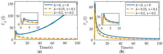
Figure 6.
Curves for energy dissipation rate under different parameters λ and γ with different sensitivities: (a) α = 1.0 and (b) α = 2.0.
Likewise, Figure 7 shows the curves for total energy dissipation E for each vehicle. It is noticeable that at low sensitivity (Figure 7a), energy dissipation E for FVD model (λ = 0, γ = 0) is characterized by rapid growth. But for GO-FVD model (λ = 0.15, γ = 0.1; λ = 0.2, γ = 0.2), the growth is relatively slow, and the energy dissipation will not increase further after a sufficiently long time. In addition, as the value of sensitivity increases to α = 2.0 (Figure 7b), the growth of E becomes slower for both FVD model and GO-FVD model. Nevertheless, energy dissipation for GO-FVD model (λ = 0.15, γ = 0.1; λ = 0.2, γ = 0.2) is still less than that for FVD model (λ = 0, γ = 0).
Figure 7.
Curves for total energy dissipation E under different parameters λ and γ with different sensitivities: (a) α = 1.0 and (b) α = 2.0.
The simulation results shown in Figure 6 and Figure 7 are consistent. It is explicit that under IoV conditions, driving strategy with consideration of Global Optimality is beneficial to suppress energy dissipation. Furthermore, as parameters λ and γ increase, energy dissipation will be reduced more significantly.
4.2.3. Applicability of GO-FVD Model
The applicability of GO-FVD model under different average headways is tested in accordance with the numerical methods in Section 3.3. The snapshots of velocity against headway (Figure 8) and position (Figure 9) at t = 4000 s are respectively displayed for the cases (a) N = 600, L = 6000 m, (b) N = 400, L = 6000 m and (c) N = 300, L = 6000 m.
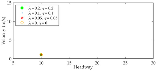
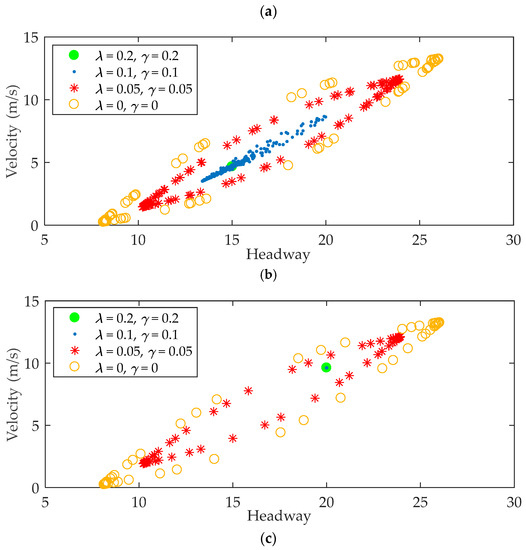
Figure 8.
Snapshots of velocity against headway under different λ and γ at t = 4000 s with α = 1.0: (a) N = 600, L = 6000 m, (b) N = 400, L = 6000 m and (c) N = 300, L = 6000 m.
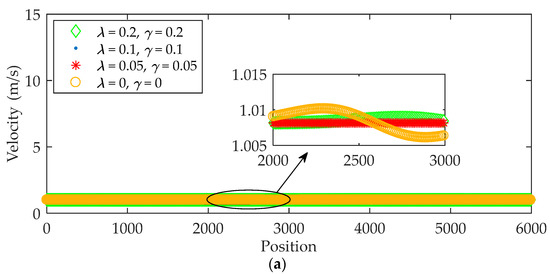
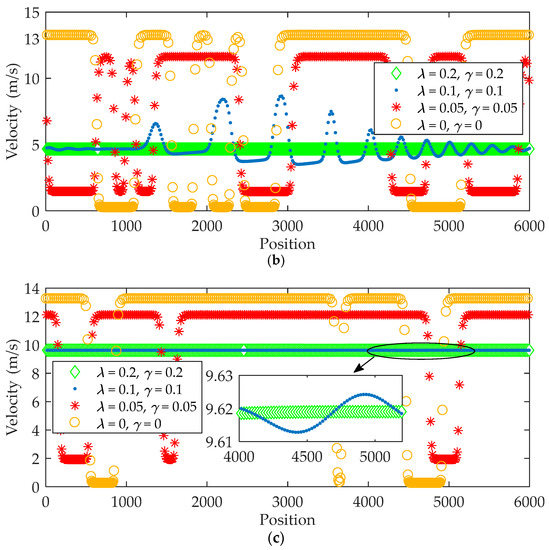
Figure 9.
Snapshots of velocity against position under different λ and γ at t = 4000 s with α = 1.0: (a) N = 600, L = 6000 m, (b) N = 400, L = 6000 m and (c) N = 300, L = 6000 m.
In Figure 8a, the average headway of traffic flow is 10 m. In this case, there seems to be only a single point, which means the velocities and headways of all vehicles show little difference as the values of parameters λ and γ change. In other words, Global Optimality has little effect on traffic flow when the average headway is 10 m. In Figure 8b, the average headway increases from 10 m to 15 m. The snapshots of velocity against headway form the approximate loops under certain value sets of λ and γ. It is found that the sizes of the approximate loops become progressively small with λ and γ increasing, indicating the traffic stability and safety are strengthened. As both λ and γ increase to 0.2 in Figure 8b, the loop shrinks to be only a point that represents the stable state. However, with the average headway increasing to 20 m in Figure 8c, the loop has shrunk to the stable point as both λ and γ just increase to 0.1. The results indicate that under larger average headway, Global Optimality plays a more active role in smoothing traffic.
Similarly, in Figure 9a, the average headway of traffic flow is 10 m. All vehicles on the whole road have similar velocities under different λ and γ. It is explicit that Global Optimality has little effect on traffic flow in this case. From Figure 9b, where the average headway increases to 15 m, one can observe that on some road segments, for instance, the positions near 1000 m or 5000 m, the velocities of vehicles approach to zero when Global Optimality is not considered (λ = 0, γ = 0). At the same time, the velocities of vehicles on some other segments, for instance, the positions near 4000 m, are more than 13 m/s when λ = 0, γ = 0. It indicates that without consideration of Global Optimality, traffic congestion may occur in some segments while drivers on some other segments may drive at a too high velocity that is unsafe. As λ and γ increase, the minimum velocity is increased, and the maximum velocity is decreased. Correspondingly, with consideration of Global Optimality, traffic congestion is alleviated, and traffic safety is improved. Particularly, when λ = 0.2 and γ = 0.2, velocities of all vehicles evolve to 4.66 m/s which is the ideal velocity for traffic flow with average headway of 15 m. In Figure 9c, where the average headway is 20 m, velocities approach to the corresponding ideal velocity when λ and γ just increase to 0.1. The results accord with those in Figure 8.
Conclusively, GO-FVD model proposed in this paper is especially suitable for the case of larger average headway, which corresponds to the low-density traffic. In this situation, taking Global Optimality into account will enhance the stability and safety of traffic flow markedly.
5. Conclusions
In this study, a hypothesis is proposed that the traffic will be improved by considering Global Optimality under IoV conditions. To investigate the effects of Global Optimality on traffic, GO-FVD model is formulated. The main improvement of GO-FVD model is that the average headway of traffic flow is selected to describe the overall situation of the traffic on a certain road. Since the average headway can be easily obtained under IoV conditions, the model is practical. Furthermore, the adverse effects of transfer delays can be weakened because the average headway of traffic flow on a certain road is relative stable information. Based on GO-FVD model, linear stability analysis and numerical simulations are conducted to explore the specific effects of Global Optimality on traffic stability, safety as well as energy dissipation.
Analytical results indicate that the stability region is enlarged in GO-FVD model, which means traffic stability is enhanced with consideration of Global Optimality. Numerical simulations agree well with analytical results. The main findings are as follows: (1) At low sensitivity, the small perturbation added to traffic flow propagates upstream in FVD model and ultimately leads to the unstable and unsafe flow. Conversely, for GO-FVD model, the perturbation is absorbed by degrees and the traffic flow returns to stable and safe state eventually. (2) At high sensitivity, traffic flow for GO-FVD model evolves to uniform flow earlier than that for FVD model. (3) Energy dissipation for GO-FVD model is explicitly less than that for FVD model. Conclusively, Global Optimality is conductive to the improvement of traffic stability and safety as well as the reduction of energy dissipation. Accordingly, these findings have verified the hypothesis proposed in the study. In addition, it is illustrated that Global Optimality plays a more active role in improving traffic with low density.
The model proposed in this study can provide theoretical reference for further study with respect to traffic problems. The findings of this study will help to support the driving tasks in the environment of IoV and promote the sustainable development of intelligent transportation. Nevertheless, there are still some limitations in the current work. In practice, weather and road characteristics will also influence the traffic, which are neglected in GO-FVD model. Noticeably, these factors are not mutually exclusive to Global Optimality. Thus, for a more realistic representation of traffic situations, GO-FVD model can be extended by accounting for these factors. Besides, the effects of Global Optimality should be tested with field data. In the current work, however, since the IoV has not been widely applied in practice, these data are lacking. Consequently, more investigations could focus on these problems in future study.
Author Contributions
All authors contributed to the work. Conceptualization, J.T.; formal analysis, L.G. and X.Q.; funding acquisition, J.T., L.G. and X.Q.; methodology, J.T. and L.G.; project administration, L.G.; resources, J.T.; software, J.T., L.G. and X.Q.; supervision, J.T.; validation, X.Q.; writing—original draft, L.G.; writing—review and editing, J.T. and X.Q.
Funding
This work was supported by the Fundamental Research Funds for the Central Universities, Zhongnan University of Economics and Law, grant number 2722019PY049, 201911403, 201911404, Soft Science Research Project of Hubei Province of China, grant number 2017ADC146 and the “New Engineering Course” Research and Practice Project of Ministry of Education of China (The Innovation and Practice of Traditional Safety Engineering Based on Simulation and Information Technology).
Acknowledgments
The authors would like to thank the School of Information and Safety Engineering, Zhongnan University of Economics and Law for providing the hardware equipment which is used to conduct simulations.
Conflicts of Interest
The authors declare no conflict of interest.
References
- Laureshyn, A.; Svensson, A.; Hydén, C. Evaluation of traffic safety, based on micro-level behavioural data: Theoretical framework and first implementation. Accid. Anal. Prev. 2010, 42, 1637–1646. [Google Scholar] [CrossRef]
- Stavrinos, D.; Jones, J.L.; Garner, A.A.; Griffin, R.; Franklin, C.A.; Ball, D.; Welburn, S.C.; Ball, K.K.; Sisiopiku, V.P.; Fine, P.R. Impact of distracted driving on safety and traffic flow. Accid. Anal. Prev. 2013, 61, 63–70. [Google Scholar] [CrossRef]
- Fotouhi, A.; Yusof, R.; Rahmani, R.; Mekhilef, S.; Shateri, N. A review on the applications of driving data and traffic information for vehicles’ energy conservation. Renew. Sustain. Energy Rev. 2014, 37, 822–833. [Google Scholar] [CrossRef]
- Tan, J.H. Rear-End Collision Risk Management of Freeways in Heavy Fog. Ph.D. Thesis, Tsinghua University, Beijing, China, June 2015. [Google Scholar]
- Liu, Y.; Yan, X.D.; Wang, Y.; Yang, Z.; Wu, J.W. Grid mapping for spatial pattern analyses of recurrent urban traffic congestion based on taxi GPS sensing data. Sustainability 2017, 9, 533. [Google Scholar] [CrossRef]
- Faria, M.; Rolim, C.; Duarte, G.; Farias, T.; Baptista, P. Assessing energy consumption impacts of traffic shifts based on real-world driving data. Transp. Res. Part D Transp. Environ. 2018, 62, 489–507. [Google Scholar] [CrossRef]
- Farooq, D.; Moslem, S.; Duleba, S. Evaluation of driver behavior criteria for evolution of sustainable traffic safety. Sustainability 2019, 11, 3142. [Google Scholar] [CrossRef]
- Torrent-Moreno, M.; Mittag, J.; Santi, P.; Hartenstein, H. Vehicle-to-Vehicle communication: Fair transmit power control for safety-critical information. IEEE Trans. Veh. Technol. 2009, 58, 3684–3703. [Google Scholar] [CrossRef]
- Knorr, F.; Schreckenberg, M. Influence of inter-vehicle communication on peak hour traffic flow. Phys. A 2012, 391, 2225–2231. [Google Scholar] [CrossRef]
- Zhang, Y.; Yang, X.G.; Liu, Q.X.; Li, C.Y. Who will use pre-trip traveler information and how will they respond? Insights from Zhongshan metropolitan area, China. Sustainability 2015, 7, 5857–5874. [Google Scholar] [CrossRef]
- Jia, R.; Jiang, P.C.; Liu, L.; Cui, L.Z.; Shi, Y.L. Data driven congestion trends prediction of urban transportation. IEEE Internet Things J. 2017, 5, 581–591. [Google Scholar] [CrossRef]
- Balasubramaniam, A.; Paul, A.; Hong, W.H.; Seo, H.; Kim, J.H. Comparative analysis of intelligent transportation systems for sustainable environment in smart cities. Sustainability 2017, 9, 1120. [Google Scholar] [CrossRef]
- Guchhait, A.; Maji, B.; Kandar, D. A hybrid V2V system for collision-free high-speed internet access in intelligent transportation system. Trans. Emerg. Telecommun. Technol. 2018, 29, e3282. [Google Scholar] [CrossRef]
- Thakur, A.; Malekian, R. Fog computing for detecting vehicular congestion, an Internet of Vehicles based approach: A review. IEEE Intell. Transp. Syst. Mag. 2019, 11, 8–16. [Google Scholar] [CrossRef]
- Alam, K.M.; Saini, M.; Saddik, A.E. Toward social Internet of Vehicles: Concept, architecture and applications. IEEE Access 2015, 3, 343–357. [Google Scholar] [CrossRef]
- Lee, E.K.; Gerla, M.; Pau, G.; Lee, U.; Lim, J.H. Internet of Vehicles: From intelligent grid to autonomous cars and vehicular fogs. Int. J. Distrib. Sens. Netw. 2016, 12. [Google Scholar] [CrossRef]
- Liu, Y.; Wu, J.; Li, J.H.; Chen, H.; Li, G.L. ISRF: Interest semantic reasoning based fog firewall for information-centric Internet of Vehicles. IET Intell. Transp. Syst. 2019, 13, 975–982. [Google Scholar] [CrossRef]
- Fernandes, P.; Nunes, U. Platooning with IVC-enabled autonomous vehicles: Strategies to mitigate communication delays, improve safety and traffic flow. IEEE Trans. Intell. Transp. Syst. 2012, 13, 91–106. [Google Scholar] [CrossRef]
- Li, Z.P.; Li, W.Z.; Xu, S.Z.; Qian, Y.Q. Analyses of vehicle’s self-stabilizing effect in an extended optimal velocity model by utilizing historical velocity in an environment of intelligent transportation system. Nonlinear Dyn. 2015, 80, 529–540. [Google Scholar] [CrossRef]
- Kuang, H.; Xu, Z.P.; Li, X.L.; Lo, S.M. An extended car-following model accounting for the average headway effect in intelligent transportation system. Phys. A 2017, 471, 778–787. [Google Scholar] [CrossRef]
- Jiang, R.; Wu, Q.S.; Zhu, Z.J. Full velocity difference model for a car-following theory. Phys. Rev. E 2001, 64, 017101. [Google Scholar] [CrossRef]
- Saifuzzaman, M.; Zheng, Z.D. Incorporating human-factors in car-following models: A review of recent developments and research needs. Transp. Res. Part C Emerg. Technol. 2014, 48, 379–403. [Google Scholar] [CrossRef]
- Pipes, L.A. An operational analysis of traffic dynamics. J. Appl. Phys. 1953, 24, 274–281. [Google Scholar] [CrossRef]
- Reuschel, A. Vehicle movements in the column uniformly accelerated or delayed. Oesterrich Ingr. Arch. 1950, 4, 193–215. [Google Scholar]
- Gazis, D.C.; Herman, R.; Rothery, R.W. Nonlinear follow-the-leader models of traffic flow. Oper. Res. 1961, 9, 545–567. [Google Scholar] [CrossRef]
- Newell, G.F. Nonlinear effects in the dynamics of car following. Oper. Res. 1961, 9, 209–229. [Google Scholar] [CrossRef]
- Kometani, E.; Sasaki, T. Dynamic Behavior of Traffic with a Nonlinear Spacing-Speed Relationship. In Proceedings of the Symposium on Theory of Traffic Flow, Research Laboratory, General Motors, New York, NY, USA, 7–8 December 1959. [Google Scholar]
- Gipps, P.G. A behavioural car-following model for computer simulation. Transp. Res. Part B Methodol. 1981, 15, 105–111. [Google Scholar] [CrossRef]
- Helly, W. Simulation of Bottlenecks in Single-Lane Traffic Flow. In Proceedings of the Symposium on Theory of Traffic Flow, Research Laboratory, General Motors, New York, NY, USA, 7–8 December 1959. [Google Scholar]
- Treiber, M.; Hennecke, A.; Helbing, D. Congested traffic states in empirical observations and microscopic simulations. Phys. Rev. E 2000, 62, 1805–1824. [Google Scholar] [CrossRef]
- Bando, M.; Hasebe, K.; Nakayama, A.; Shibata, A.; Sugiyama, Y. Dynamical model of traffic congestion and numerical simulation. Phys. Rev. E 1995, 51, 1035–1042. [Google Scholar] [CrossRef]
- Helbing, D.; Tilch, B. Generalized force model of traffic dynamics. Phys. Rev. E 1998, 58, 133–138. [Google Scholar] [CrossRef]
- Andersen, G.J.; Sauer, C.W. Optical information for car following: The driving by visual angle (DVA) model. Hum. Factors J. Hum. Factors Ergon. Soc. 2007, 49, 878–896. [Google Scholar] [CrossRef]
- Kikuchi, C.; Chakroborty, P. Car following model based on a fuzzy inference system. Transp. Res. Rec. J. Transp. Res. Board 1992, 1365, 82–91. [Google Scholar]
- Biswas, S.; Tatchikou, R.; Dion, F. Vehicle-to-vehicle wireless communication protocols for enhancing highway traffic safety. IEEE Commun. Mag. 2006, 44, 74–82. [Google Scholar] [CrossRef]
- Ibáñez, J.A.G.; Zeadally, S.; Contreras-Castillo, J. Integration challenges of intelligent transportation systems with connected vehicle, cloud computing, and Internet of Things technologies. IEEE Wirel. Commun. 2015, 22, 122–128. [Google Scholar] [CrossRef]
- Talebpour, A.; Mahmassani, H.S. Influence of connected and autonomous vehicles on traffic flow stability and throughput. Transp. Res. Part C Emerg. Technol. 2016, 71, 143–163. [Google Scholar] [CrossRef]
- Qin, Y.Y.; Wang, H.; Wang, W.; Ni, D.H. Review of car-following models of adaptive cruise control. J. Traffic Transp. Eng. 2017, 17, 121–130. (In Chinese) [Google Scholar]
- Kesting, A.; Treiber, M.; Schönhof, M.; Kranke, F.; Helbing, D. Jam-Avoiding Adaptive Cruise Control (ACC) and Its Impact on Traffic Dynamics. In Traffic and Granular Flow’05; Schadschneider, A., Pöschel, T., Kühne, R., Schreckenberg, M., Wolf, D.E., Eds.; Springer: Berlin, Germany, 2007. [Google Scholar]
- Kesting, A.; Treiber, M.; Helbing, D. Enhanced intelligent driver model to access the impact of driving strategies on traffic capacity. Philos. Trans. A Math. Phys. Eng. Sci. 2010, 368, 4585–4605. [Google Scholar] [CrossRef]
- Monneau, R.; Roussignol, M.; Tordeux, A. Invariance and homogenization of an adaptive time gap car-following model. Nonlinear Differ. Equ. Appl. 2014, 21, 491–517. [Google Scholar] [CrossRef][Green Version]
- Hua, X.D.; Wang, W.; Wang, H. A car-following model with the consideration of vehicle-to-vehicle communication technology. Acta Phys. Sin. 2016, 65. (In Chinese) [Google Scholar] [CrossRef]
- Wang, T.; Gao, Z.Y.; Zhao, X.M. Multiple velocity difference model and stability analysis. Acta Phys. Sin. 2006, 55, 634–640. (In Chinese) [Google Scholar]
- Peng, G.H.; Sun, D.H. A dynamical model of car-following with the consideration of the multiple information of preceding cars. Phys. Lett. A 2010, 374, 1694–1698. [Google Scholar] [CrossRef]
- Sun, Y.Q.; Ge, H.X.; Cheng, R.J. An extended car-following model under V2V communication environment and its delayed-feedback control. Phys. A 2018, 508, 349–358. [Google Scholar] [CrossRef]
- Nakayama, A.; Sugiyama, Y.; Hasebe, K. Effect of looking at the car that follows in an optimal velocity model of traffic flow. Phys. Rev. E 2002, 65, 016112. [Google Scholar] [CrossRef]
- Tan, J.H.; Shi, J. Impact of intermittent vehicle release on freeway energy dissipation and emissions. J. Tsinghua Univ. (Sci. Technol.) 2013, 53, 499–502. (In Chinese) [Google Scholar]


© 2019 by the authors. Licensee MDPI, Basel, Switzerland. This article is an open access article distributed under the terms and conditions of the Creative Commons Attribution (CC BY) license (http://creativecommons.org/licenses/by/4.0/).