Long- and Short-Run Effects of Fuel Prices on Freight Transportation Volumes in Shanghai

Abstract

Freight transportation modes consume enormous amounts of energy. This paper estimates the long- and short-run effects of fuel prices on freight volumes in various modes of transportation in Shanghai. Data included monthly changes during the period 2009–2016. Air cargo series were suggested to include one or two unit roots, and hence were removed from the cointegration analysis. Both the Phillips–Ouliaris and Johansen tests did not detect long-run relationships between real fuel prices, water cargo, road, and rail freight. Conventional first-differenced VAR (vector autoregressive) models were estimated. Overall, whether in the short- or long-run, real fuel prices did not influence freight transportation volumes. However, we found a Granger causality running from rail to road freight, as in the short-run (one month), a 1% change in rail freight would lead to a reduction of 0.07% in road freight. Therefore, simply by increasing fuel prices, the government could seldom encourage the shift from energy-inefficient modes of freight transportation to energy-efficient ones to achieve a sustainable freight transport. The allocation of more time and routes for rail freight traffic and the reduction in rail freight taxes may increase the rail freight volume and hence decrease the overall energy use. Our findings, to some degree, contribute to freight transportation economics. Future research may examine the impact of gasoline prices or diesel prices on freight traffic volumes.

1. Introduction

In 2006 and 2017, 726.2 million and 972.6 million tons were transported in Shanghai, respectively [1]. Of the 972.6 million tons of total freight traffic volume in 2017, waterway accounted for 58.2%, 6.7 percentage points higher than in 2006, and air accounted for 0.43%, 0.08 percentage points higher than in 2006. However, road accounted for 40.9%, 5.6 percentage points less than in 2006, while rail accounted for 0.49%, 1.18 percentage points less than in 2006. Hence, during the period 2006–2017, waterway transportation increased significantly, and air grew slightly, whereas both road and rail had a dramatic reduction.

We argue that fuel cost is a determinant of freight traffic demand in Shanghai. In 2017, Shanghai consumed 118.6 million TCE (tons of coal equivalent) of energy, with industrial and residential consumption accounting for 48.2% and 11.6%, respectively. The transportation, warehousing, post, and telecommunications sector accounted for 21.7% [2]. Additionally, during the period 2010–2016, the freight traffic volume in Shanghai grew by 9.46%; however, diesel consumption in the transportation, warehousing, post, and telecommunications sector grew by 28%. Hence, the growth in truck capacity and diesel consumption greatly exceeded the increase in freight volume. In terms of diesel use, freight transportation in Shanghai seems to be energy-inefficient.

We take freight traffic volume (in tons) as a proxy for freight traffic demand. Hence, changes in fuel prices may impact traffic volumes in various modes of freight transportation (waterway, road, rail, and air). This paper examines the long- and short-run effects of fuel prices on freight volumes in Shanghai. We anticipate that our tests would provide empirical evidence for whether we can adopt a fuel price policy to realize the shift from energy-inefficient modes of freight transportation to energy-efficient ones.

The remainder of this paper is organized as follows. Section 2 reviews the literature, and Section 3 briefly presents the methods used. Section 4 describes the data, while Section 5 reports the econometric results. Section 6 discusses some of the significant results, and finally Section 7 summarizes the conclusions.

2. Literature Overview

Freight transportation is an energy-intensive sector. In the U.S., the freight transportation sector accounts for approximately 6.8% of the national energy consumption [3]. In 2017, Shanghai’s transportation, postal services, and information transmission together accounted for about 21.7% of the overall energy consumption [2].

Therefore, there may be a close relationship between fuel prices and freight volumes in various modes of freight transportation. Literature on the fuel price elasticity of freight demand is mixed, which may result in different price policies. Freight demand is often fuel price inelastic. For example, the U.S. trucking sector is relatively fuel price inelastic [4], with single-unit truck activity not being sensitive to diesel fuel prices over the period 1980–2012 [5], as higher fuel prices in the trucking industry slightly reduced fuel use [6]. Additionally, light goods vehicles and articulated trucks did not respond to changes in fuel prices in the UK. Hence, price-based policies that were designed to reduce fuel demand from light vehicles could not be effective [7], and fuel price did not appear to be an effective instrument for reducing energy demand in freight transport [8].

However, some studies suggest that freight demand is fuel price elastic; heavy goods vehicles and rigid trucks were fuel price elastic in the UK [7]. If rail capacity is sufficient, an apparent increase in fuel prices could cause a shift from truck to rail, which might result in a 30% reduction in fuel consumption by 2050 [9]. Moreover, fuel prices had certain effects on the traffic level [10]. If fuel prices have a significant effect on freight transport modes, we can anticipate that the price policy could cause a shift from energy-inefficient modes to energy-efficient modes. For example, to reduce freight energy use, Komor [11] suggested shifting from truck to rail by increasing freight fuel prices. Income is a powerful determinant of the long-run behavior of the U.S. airfreight industry. U.S. airfreight is income elastic [12].

Relative energy efficiency differs between various modes of freight transportation. For example, in terms of energy per ton mile, oil pipelines are the most energy-efficient, followed by railway, road, and cargo planes [13]. In addition, although rail freight is very energy efficient [14], waterway freight services are more energy-efficient than both rail and road [15]. Overall, compared with road traffic, rail traffic could save nearly 35% energy consumption [16]. Railway and waterway distribution are more environmentally sustainable than truck distribution and are thereby being encouraged by policies [17]. Hence, in freight networks, it is economically attractive to bundle demand over modes that have large vehicle and infrastructure capacity, such as barges or rail [18].

3. Methods

To detect the long-run relationships between energy prices and freight, the Phillips–Ouliaris test could provide clues to the cointegration [19]. We estimated the trace statistics and cointegrating vector(s) [20,21]. In the trace tests, we conducted finite-sample Cheung–Lai critical-value corrections [22] and trace corrections [23].

We tested for unit root, utilizing the ADF (augmented Dickey–Fuller) and the PP (Phillips–Perron) techniques [24,25]. Also, we conducted the ERS DF-GLS (Elliott–Rothenberg–Stock Dickey–Fuller generalized least squares) tests. To obtain preferable power and size properties in finite samples, the ERS DF-GLS test applies the GLS technique to detrend data and selects the lag length using the MAIC (modified Akaike information criterion) [26].

Moreover, a structural break (or outlier) existing in data may lead to incorrect inferences for unit roots [27,28]. The means of the variables were non-zero (

Table 1. Statistics and variables.

Variable	RFP	WATER	ROAD	RAIL	AIR
Description	Real Fuel Price Defined as the Price Index of Fuels and Power Divided by CPI	Waterway Cargo Volume	Truck Freight Traffic Volume	Rail Freight Traffic Volume	Air Freight Traffic Volume
Mean	0.93	3826.91	3443.39	60.19	29.12
Median	0.92	3948.50	3512.34	61.70	29.33
Maximum	1.47	5042.09	3828.23	84.10	35.30
Minimum	0.63	2788.01	2969.10	35.58	20.40
Std. Dev.	0.19	483.98	183.17	16.75	2.68
Skewness	0.55	−0.22	−0.60	−0.11	−0.90
Kurtosis	3.08	2.85	2.55	1.42	4.44
Jarque–Bera	4.88	0.86	6.54	10.19	21.32
Probability	0.09	0.65	0.04	0.01	0.00
Data type	Time series
Frequency	Monthly
Period of study	January 2009 to December 2016
Seasonally adjustment	X-12 (additive)

Notes: Freight measurement—10,000 tons.

) and data appeared to include the trend (Figure 1). Hence, the Perron break date tests were driven, utilizing the mixed IO (innovational outlier) model [29]. The Perron structural break test allows for both level and slope shifts to take place simultaneously in the IO Model C. Model C is recommended when the break date is taken as unknown [30]. The Perron IO Model C is:

$$y_{\mathrm{t}}=\mu +\theta D{U}_{\mathrm{t}}+\beta t+\gamma D{T}_{\mathrm{t}}+\delta D{\left(TB\right)}_{\mathrm{t}}+\alpha y_{\mathrm{t}-1}+{\sum }_{i=1}^k{c}_{\mathrm{i}}\Delta y_{\mathrm{t}-i}+{\epsilon }_{\mathrm{t}},$$

(1)

where DU_t allows for a one-time change in the intercept of the trend function, DU_t = 1 if t > T_b and 0 otherwise. T denotes the sample size and T_b is the break date to be selected. DT_t allows for a change in the slope of the trend function, DT_t = t if t > T_b and 0 otherwise. D(TB), the one time dummy, equals 1 if t = T_b + 1 and 0 otherwise.

The $t_{\alpha }$-value on α was used to evaluate the null hypothesis. Under the null hypothesis of a unit root, $\theta =0$ (except in Model C), $\beta =0$, $\gamma =0$, $\alpha =1$. $\delta \ne 0$, particularly it should be significantly different from zero. Under the alternative hypothesis of a trend stationary process, $\theta \ne 0$, $\beta \ne 0$, $\gamma \ne 0$ (in general), $\delta =0$ and $\alpha <1$.

We could construct an ECM (error-correction model), where cointegration existed. However, if the series were integrated of order one, but not cointegrated, traditional VAR (vector autoregressive) models were valid [31]. In the ECM or VAR models, short-run and long-run effects in terms of elasticity and Granger causality were suggested [31,32,33]. A conventional VAR can be formulated as:

$$\mathsf{\Delta }{y}_{\mathrm{t}}={\delta }_1\mathsf{\Delta }{y}_{\mathrm{t}-1}+\dots +{\delta }_k\mathsf{\Delta }{y}_{\mathrm{t}-k}+{\epsilon }_{\mathrm{t}},$$

(2)

where y_t represents a set of I(1) variables, while μ denotes the intercept. k denotes the lag order, and ε_t represents the white noises with zero mean and finite variance. Working with the estimated VAR, we could conduct a conventional Granger causality test using the Wald χ²-statistic. Using variables in logarithms, coefficient δ was interpreted as short-run elasticity, which was economically significant.

4. Data

We used monthly series for the period from January 2009 to December 2016. The PIFP (price index of fuels and power) was the most significant indicator of changes in energy prices in Shanghai, a component of the industrial producer’s purchase price, and reflected changes in prices of representative energy products that companies purchased. Representative energy products included coal, gasoline, diesel, kerosene, natural gas, and power.

In the online Shanghai Statistics’ Data Release, under item 7 (prices) and Section 3 (industrial producers’ purchase price index), the PIFP series are reported monthly, which are measured using the nominal index change over the same month of the previous year [34]. We used RFP (real fuel prices), which were obtained by dividing the PIFP index by the CPI (Shanghai consumer price index). The CPI was calculated by taking price changes over the same month of the previous year. In the online Shanghai Statistics’ Data release, under item 7 (prices), and Section 1 (consumer price index), the CPI series are reported monthly [35].

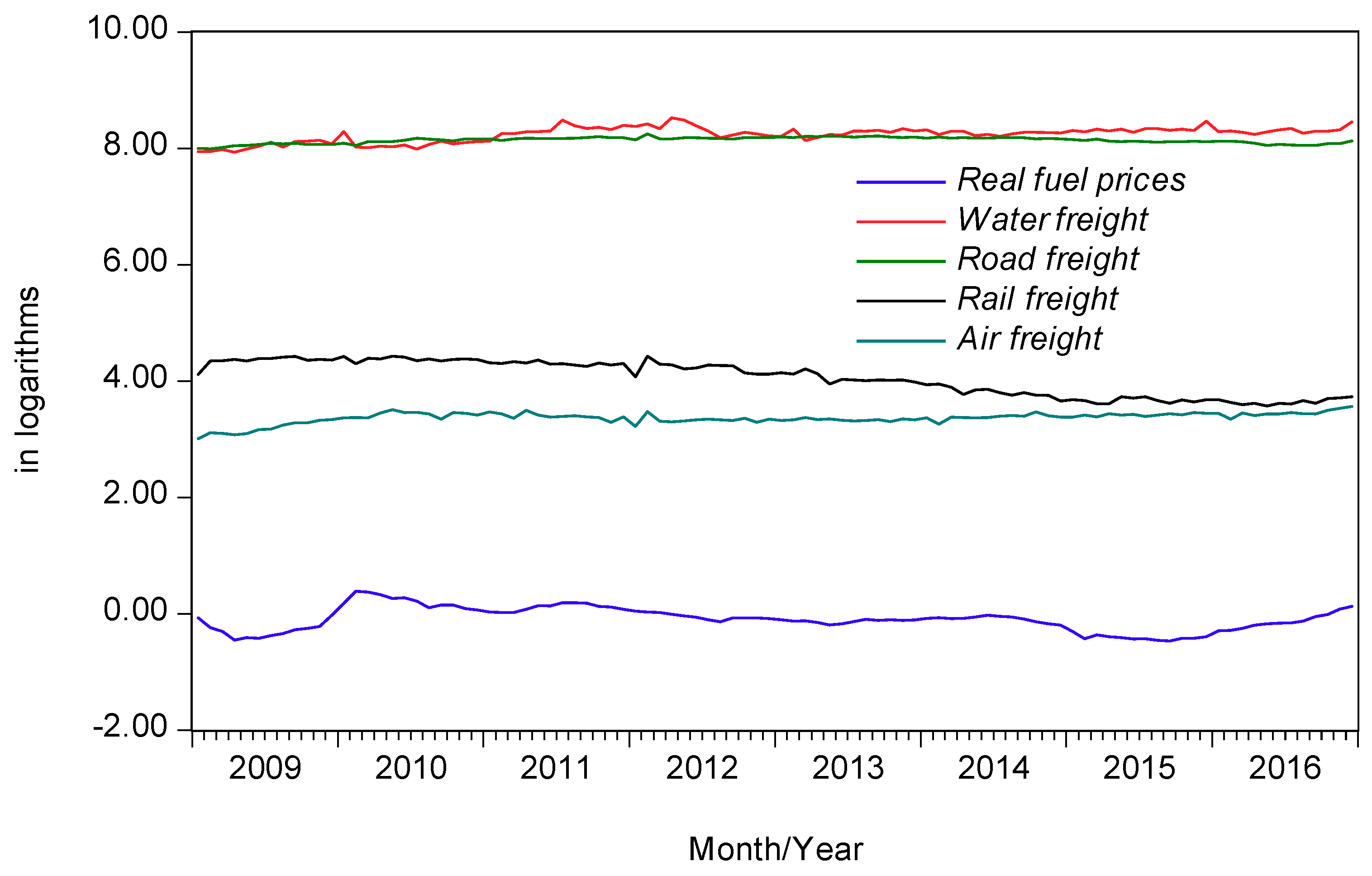
In the online Shanghai Statistics’ Data Release, under item 6 (service sector) and Section 2 (transportation), the freight transportation volume series are reported monthly. Shanghai Statistics divide freight volume into four types: WATER (waterway cargo), ROAD (road freight), RAIL (rail freight), and AIR (air cargo) [36]. Table 1 statistically describes the data, and Figure 1 plots the changes in freights and real fuel prices in Shanghai.

We could accept the normality for waterway cargo volume, real fuel prices, and road and rail freight volumes at the 10%, 5%, and 1% levels, respectively. However, normality for air freight volume was rejected at the 1% level, as a kurtosis of 4.44 for this series may have undermined the normality.

5. Empirical Results

Although the ADF tests indicated no unit root for RFP, the PP tests indicated one, with the ERS DF-GLS tests suggesting at least two unit roots for this variable (

Table 2. The unit root tests.

	k	Level	p-Value	k	First Difference	p-Value	k	Second Difference
Variable	ADF
RFP	7	−3.76 **	0.02	−	−	−	−	−
WATER	1	−2.78	0.21	1	−8.85 ***	0.00	−	−
ROAD	9	−2.31	0.42	10	−3.30 *	0.07	−	−
RAIL	3	−2.24	0.46	6	−3.37 *	0.06	−	−
AIR	11	−2.20	0.49	7	−2.04	0.57	9	−5.84 ***
	PP
RFP	5	−2.00	0.59	2	−6.16 ***	0.00	−	−
WATER	2	−3.55	0.04	6	15.45	0.00	−	−
ROAD	5	−2.63	0.27	3	−15.96 ***	0.00	−	−
RAIL	1	−5.07	0.00	−	−	−	−	−
AIR	3	−4.27 ***	0.01	−	−	−	−	−
	ERS DF-GLS
RFP	1	−2.41	−	3	−2.11	−	9	−0.79
WATER	2	−1.92	−	10	−1.67	−	11	−1.24
ROAD	11	−1.03	−	11	−1.09	−	9	−1.77
RAIL	3	−0.92	−	6	−1.09	−	6	−1.87
AIR	2	−1.07	−	7	−0.58	−	6	−2.20

Notes: Data were seasonally adjusted using the X-12 (additive) technique and logarithms. All tests included an intercept as well as a trend, based on Figure 1 and according to [37,38]. The lag length k was selected using the t-statistic for the ADF test [39]. k was determined using the Newey–West (NW) bandwidth technique for the PP test [40]. k was chosen using the modified AIC (MAIC) for the ERS DF-GLS test [41]. In this test, MAIC is suggested to dominate all other criteria [26]. The p-value denotes MacKinnon’s p-value [42]. *, ** and *** denote rejection of the null hypothesis of a unit root at the 10%, 5%, and 1% levels, respectively.

). The existence of a structural shift in RFP may increase the variable order (

Table 3. The Perron structural break tests using the IO (innovational outlier) Model C.

Variable	Parameter	Coefficient	Standard Error	t-Statistic	p-Value	Tb
RFP	θ	−1.19	0.28	−4.32	0.00	June 2015
	β	0.00	0.00	−4.39	0.00
	γ	0.01	0.00	4.45	0.00
	δ	0.04	0.05	0.72	0.47
	α	0.69	0.08	8.84	0.00
	Intercept	0.10	0.02	4.07	0.00
	k = 11	Adj. R2 0.96	F-stat. 122	DW-stat. 2.09
WATER	θ	0.35	0.10	3.42	0.00
	β	0.01	0.00	4.24	0.00
	γ	−0.01	0.00	−3.99	0.00
	δ	−0.08	0.07	−1.16	0.25
	α	0.06	0.21	0.30	0.77
	Intercept	7.36	1.65	4.47	0.00
	k = 10	Adj. R2 0.69	F-stat. 13.3	DW-stat. 2.05
ROAD	θ	0.11	0.05	1.98	0.05
	β	0.00	0.00	0.87	0.39
	γ	0.00	0.00	-2.06	0.04
	δ	-0.01	0.02	-0.34	0.74
	α	0.62	0.14	4.50	0.00
	Intercept	3.08	1.12	2.76	0.01
	k = 9	Adj. R2 0.85	F-stat. 34.4	DW-stat. 2.09
RAIL	θ	−0.61	0.16	−3.84	0.00	June 2014
	β	0.00	0.00	−2.34	0.02
	γ	0.01	0.00	4.01	0.00
	δ	0.00	0.07	0.06	0.95
	α	0.88	0.16	5.55	0.00
	Intercept	0.61	0.72	0.84	0.40
	k = 10	Adj. R2 0.96	F-stat. 144	DW-stat. 2.00
AIR	θ	−0.19	0.08	−2.37	0.02
	β	0.00	0.00	−1.90	0.06
	γ	0.00	0.00	2.87	0.01
	δ	0.02	0.05	0.41	0.69
	α	0.36	0.17	2.14	0.04
	Intercept	2.19	0.58	3.74	0.00
	k = 11	Adj. R2 0.53	F-stat. 6.89	DW-stat. 1.92

Notes: Variables are in logarithms. Test equations included a slope and an intercept. We selected the lag order k (between 2 and 12) using a general-to-specific recursive procedure. This procedure is data-dependent. A t-statistic in absolute value on the last lagged term must be greater than or equal to 1.80. This method can have few size distortions and/or less power losses with data in the class of ARMA (autoregressive moving average) processes [29,39]. The trimming fraction λ was 0.15. λ was suggested to be 0.15 [43]. The critical values for a sample size of 100 were −6.21, −5.55, −5.25 at the 1%, 5%, and 10% levels, respectively [29]. T_b is the selected structural break time.

). We know that under the null hypothesis of a unit root, α = 1, $\mathrm{intercept}\ne 0$ (in general), β = 0, γ = 0, δ ≠ 0 [29]. In this case, α ≈ 1 (0.68), $\mathrm{intercept}\ne 0$. Hence, we suggest that RFP is a near I(1) variable.

Similarly, although the ADF tests indicated a unit root for RAIL, the PP tests indicated none, with the ERS DF-GLS tests suggesting at least two unit roots for this variable. The existence of a structural break in RAIL may increase the variable order. In this case, α ≈ 1 (0.88) (Table 3). Hence, we suggest that RAIL is a near I(1) variable.

Both the ADF and PP tests indicated one unit root for both WATER and ROAD. In addition, break date tests suggested a unit root for these two variables. Hence, we suggest that both WATER and ROAD are I(1), although the ERS DF-GLS tests suggested at least two unit roots for them.

Although the ADF tests suggested two unit roots for AIR, the PP tests suggested none, with the ERS DF-GLS tests suggesting at least two unit roots for this variable. The break date tests suggested a unit root for this variable. Thus, AIR may contain one or two unit roots.

We removed the variable AIR from the subsequent cointegration analysis, as it possibly included one or two unit roots and had unsatisfactory normality properties. We first tested for multivariate cointegration for the variable set RFP, WATER, ROAD, and RAIL using the lag lengths k = 2, 3, 4, 5, 6, 7, and 8 (

Table 4. The Johansen multivariate cointegration trace tests.

k	r	Trace	Asymptotical Critical Value *	Cheung–Lai Correction **	Reinsel–Ahn Correction ***	Multivariate Normality (p-Value)	Adj. Q (p-Value, Lags)
2	0	58.99	63.88	69.09	52.85	220(0.00)	172(0.51, 12)
	≦1	36.59	42.92	46.42	32.78
	≦2	17.00	25.87	27.98	15.23
	≦3	3.86	12.52	13.54	3.46
3	0	57.92	63.88	72.04	48.87	196(0.00)	154(0.54, 12)
	≦1	33.67	42.92	48.40	28.41
	≦2	15.41	25.87	29.18	13.00
	≦3	4.03	12.52	14.12	3.40
4	0	59.43	63.88	75.30	47.05	198(0.00)	153(0.23, 12)
	≦1	32.50	42.92	50.59	25.73
	≦2	16.11	25.87	30.50	12.75
	≦3	4.63	12.52	14.76	3.66
5	0	64.19	63.88	78.89	47.48	201(0.00)	145(0.11, 12)
	≦1	32.10	42.92	53.01	23.74
	≦2	15.90	25.87	31.96	11.76
	≦3	6.65	12.52	15.46	4.92
6	0	67.78	63.88	82.89	46.60	207(0.00)	131(0.08, 12)
	≦1	37.50	42.92	55.69	25.78
	≦2	16.77	25.87	33.57	11.53
	≦3	7.37	12.52	16.24	5.06
7	0	80.91	63.88	87.36	51.41	193(0.00)	134(0.00, 12)
	≦1	49.18	42.92	58.69	31.25
	≦2	27.04	25.87	35.38	17.18
	≦3	8.75	12.52	17.12	5.56
8	0	90.27	63.88	92.38	52.66	183(0.00)	172(0.00, 12)
	≦1	54.44	42.92	62.07	31.76
	≦2	27.60	25.87	37.42	16.10
	≦3	8.03	12.52	18.10	4.68

Notes: Variables are in logarithms. * denotes the 5% asymptotical critical value [45]. ** denotes the Cheung–Lai finite-sample critical value [22]. *** denotes the Reinsel–Ahn trace correction [23]. The multivariate normality Jarque–Bera statistic was estimated using the inverse square root of residual covariance matrix [46]. Adj. Q denotes the Portmanteau autocorrelation test adjusted Q-statistic.

). We used assumption IV, following the recommendation by [44]. In all cases, a multivariate normality did not exist. The k = 7 and 8 cases included autocorrelations. Of the remaining k = 2, 3, 4, 5, 6 cases, the k = 2 case minimized the AIC (Akaike information criterion) and SIC (Schwarz information criterion). Hence, we chose the k = 2 case as the final test, which suggested no cointegration. In addition, Phillips–Ouliaris tests did not suggest cointegration (

Table 5. Phillips–Ouliaris tests.

Log of Dependent Variable	Zα-Statistic	p-Value *	Haug‘s Criticle Value **
RFP	−15.60	0.49	−38.25
WATER	−24.85	0.12
ROAD	−12.42	0.67
RAIL	−9.45	0.83

Notes: The null hypothesis was that the series did not include a cointegrating vector. Lags were chosen as per AIC. * denotes that the p-values followed [42]. ** Haug provided critical values for the Z_α Phillips–Ouliaris test in small samples [47].

). Finally, we suggest that these four variables were not cointegrated.

Therefore, we estimated the conventional first-differenced VAR models for the variable set RFP, WATER, ROAD, and RAIL, and selected an optimal lag length of 1 for the VAR using various criteria (

Table 6. Lag selection for the VAR (vector autoregressive) model.

Lag	LR	AIC	SIC	HQ
0	−	−12.71	−12.60	−12.66
1	87.27 *	−13.40 *	−12.83 *	−13.17 *
2	14.66	−13.23	−12.21	−12.82
3	12.82	−13.03	−11.56	−12.44
4	13.22	−12.85	−10.93	−12.08
5	18.90	−12.77	−10.39	−11.81
6	16.91	−12.68	−9.84	−11.53
7	21.76	−12.68	−9.40	−11.36
8	14.97	−12.59	−8.85	−11.09

Notes: LR denotes LR test statistics at the 5% level. AIC is the Akaike information criterion, while SIC is the Schwarz information criterion. HQ is the Hannan–Quinn information criterion. * indicates statistics that were used to select the ‘optimal’ lag order.

). The estimated VAR models passed the autocorrelation and F-tests (

Table 7. Estimates of the first-differenced VAR models.

	Dependent
Lagged Variable	RFP	WATER	ROAD	RAIL
RFP(−1)	0.47(5.32) *	−0.14(−1.19)	0.01(0.35)	−0.02(−0.16)
WATER(−1)	0.12(1.60)	−0.39(−4.02) *	−0.02(−0.79)	−0.13(−1.50)
ROAD(−1)	−0.16(−0.59)	−0.52(−1.47)	−0.31(−2.92) *	−0.20(−0.61)
RAIL(−1)	0.11(1.39)	−0.06(−0.55)	−0.07(−2.04) *	−0.38(−3.82) *
Constant	0.00(0.63)	0.01(1.06)	0.00(0.71)	−0.01(−1.17)

Notes: * indicates significant estimates. t-statistics are in parentheses. Data were transformed into logarithms and first differenced. Multivariate normality Jarque–Bera: 244 (p-value = 0.00) [46]. Adj. Q: 21 (p-value = 0.2, lag = 2). Adj. R²: 0.23. F-statistic: 7.76.

). In addition, utilizing the estimates for the conventional VAR models, we conducted the Granger causality tests (

Table 8. Granger causality tests.

Dependent Variable	Excluded Lagged Variables	Chi-Square	Degree of Freedom	p-Value
RFP	WATER	2.55	1	0.11
	ROAD	0.35	1	0.55
	RAIL	1.93	1	0.16
WATER	RFP	1.41	1	0.24
	ROAD	2.15	1	0.14
	RAIL	0.30	1	0.58
ROAD	RFP	0.12	1	0.73
	WATER	0.63	1	0.43
	RAIL	4.17	1	0.04 *
RAIL	RFP	0.03	1	0.87
	WATER	2.26	1	0.13
	ROAD	0.38	1	0.54

Notes: Tests were based on VAR estimates in Table 7. * indicates rejection of the non-Granger causality null hypothesis at the 5% level.

), with only one causal relationship being suggested at the 5% level, RAIL Granger caused ROAD. The estimated coefficient of the effect of RAIL on ROAD was −0.07 and statistically significant, which implies that in the short-run (one month), a 1% change in rail freight would lead to a reduction of 0.07% in road freight. In particular, estimates for the effects of RFP on WATER, ROAD, and RAIL were statistically insignificant. No Granger causality existed from RFP to WATER, ROAD, and RAIL. Therefore, in the short-run, real fuel prices did not influence freight volumes in various transportation modes.

6. Discussion

The cointegration analysis did not find long-run relationships between real fuel prices and freight volumes in Shanghai. We argue that because of the government-controlled energy prices, the changes in fuel prices are distorted in the market. Hence, freight demand in various modes of freight transportation has considered fuel prices less than otherwise. Substantial evidence supports government-controlled energy prices [48,49,50,51]. In particular, during the period 2010–2012, world crude oil prices at the 2018 constant dollar increased by 33.4% [52], while in Shanghai, prices of fuels and power at the 2000 constant price increased by only 16.6% [53], which is 16.8 percentage points less than the world oil price’s growth. During the period 2012–2017, world crude oil prices in constant terms declined by 54.5%, while Shanghai’s prices of fuels and power declined by 35.7%, which is 18.8 percentage points less than the reduction in world oil price. Conversely, we argue that the freight volume largely reflects the real market demand. Therefore, it is difficult to form a long-run balanced interaction between controlled fuel prices and the market-oriented freight volume.

The second reason for the nonexistence of long-run relationships is due to some specific characteristics of the goods, part of the freight could rarely shift between the modes of freight transportation (water, road, rail, and air) with fuel prices. For example, Shanghai is a coastal city located at the mouth of the Yangtze River; thus, a large number of aquatic products are transported by water and road, but are difficult to transport by air and rail. Shanghai’s urban construction has grown rapidly, generating a large amount of construction waste. This construction waste is mainly transported by road using heavy-duty vehicles. In addition, hazardous chemicals are mainly transported by road, while gasoline and diesel are mainly transported by road and rail. Natural gas is mainly transported by pipelines and water. However, the growth in volume of these different modes of freight transportation is extremely nonproportional. In the case that the freight volume (demand) could rarely adjust various modes of freight transportation to fuel prices, it is difficult to form a long-run equilibrium between the modes, and between the prices and transportation modes.

Fuel prices have no short-run effects on freight transportation volumes for the same reasons, including specific characteristics of some goods, large quantities, and fixed modes of transportation. Thus, whether in the long- or short-run, they have relatively fixed modes of transportation, which rarely respond to changes in energy prices. In addition, given the massive amount of transported goods, in the short term, freight transportation could not respond to changes in fuel prices; hence, the demand for freight transportation is often inelastic relative to fuel prices.

In recent years, the capacity of Shanghai trucks has increased significantly, which might lead to excess road capacity. For example, during the period 2010–2016, although the freight transportation volume increased by only 9.46%, the number of trucks increased by 21.7%, and the truck capacity increased by 22.8% [53]. Out of survival, trucks compete with each other for freight, regardless of fuel costs; hence, fuel prices have little effect on their shipments.

The finding that fuel prices has little effect on freight volume contributes to transportation economics to some extent, and is consistent with some studies [4,5,7]. However, compared to past studies, we disaggregated the impact of fuel prices on freight transportation into the short- and long-run. The long-run impact has more economic and policy significance than the short-run.

Overall, fuel prices have neither long- nor short-run effects on the transportation of goods. These findings have significant implications for sustainable energy use and macroeconomics. For example, we can rarely shift from energy-inefficient modes of freight transportation (e.g., roads) to energy-efficient modes (e.g., rail and water) by merely raising fuel prices.

Another interesting finding is that railway freight Granger caused road freight. In the short-run, an increase of 1% in rail freight would lead to a decline of 0.07% in road freight. Hence, rail freight has a short-run substitution for road freight, although this substitution effect is relatively weak. Since rails are more energy-efficient than highways, our findings have implications for improving the energy efficiency of freight transportation and achieving sustainable freight transportation.

During the period 2000–2016, the mileage of road transportation in Shanghai increased by 122.6%, while road freight and passenger transportation increased by 37.7% and 37.1%, respectively. Railway transportation mileage increased by 80.9%, while railway freight volume decreased by 56.3%, and railway passenger transportation increased by 256%. Therefore, the railway capacity has been excessively allocated to passenger traffic. Although in the short-run, rail freight has a certain substitution for road freight, this substitution has been weakened due to the shortage of rail freight capacity. Since fuel prices, as defined in this research, could rarely influence freight volumes, we suggest that the government could use appropriate policies to increase rail freight transportation, while decreasing road freight. Policies may include the allocation of more time and routes for rail freight traffic and the reduction in rail freight taxes.

7. Conclusions

Freight transportation consumes a considerable amount of energy. This paper examined the effects of fuel prices on the freight traffic volumes in the water, road, rail, and air modes in Shanghai. The data were monthly series for the period 2009–2016. We tested for unit root using the ADF, PP, and ERS DF-GLS techniques. In addition, we conducted the Perron’s break date tests. The air freight series included one or two unit roots and were accordingly removed from the cointegration analysis. We tested for cointegration using both the Johansen and Phillips–Ouliaris tests.

Tests did not find a long-run equilibrium between real fuel price (index) and freight volumes in the water, road, and rail modes. We attribute this to government-controlled energy prices and specific characteristics of the goods, which make them dependent on one or two relatively fixed freight modes.

We estimated the conventional first-differenced VARs, with no Granger causal relationships between real fuel prices and the volumes of water, road, and rail freight transportation.

Tests suggested that in the short-run, an increase of 1% in rail freight would lead to a decline of 0.07% in road freight. Hence, rail freight has a slight short-run substitution for road freight. This finding may benefit sustainable freight transportation.

Overall, the real fuel prices lack long- as well as short-run links with freight demand in Shanghai. Our findings are consistent with some of the literature, and therefore could contribute to the freight transportation economics to some extent.

Regarding macroeconomic policies, governments could hardly promote the shift between modes of freight transportation to achieve sustainable energy-efficient freight transport, simply by raising fuel prices. Additionally, railway capacity has been excessively allocated to passengers. Policies that include the allocation of more time and routes for rail freight traffic and the reduction in rail freight taxes may increase rail freight transportation and decrease the overall energy use.

However, the energy price data we used were an average energy price index (PIFP) for various energy products. If gasoline prices or diesel price data are available, we recommend that future research could analyze the impact of these specific fuel prices on freight traffic volume. The results of the potential study can be easily compared with previous research results, e.g., [4,5,7]. In addition, the freight volume may be endogenous relative to the energy price, and vice versa. Freight volumes between various modes of transportation may also be endogenous relative to each other; for example, this study found that in the short-run, road freight is endogenous relative to rail freight. We recommend that future research may construct an SVAR (structural vector autoregressive) model to analyze the relationship between fuel prices and freight volume.