Abstract
An industrial system has positive and negative strategies to adapt to environmental regulations, which can be defined as natural disposability and managerial disposability. Meanwhile, the operational process of an industrial system can be divided into regular production activities and pollutant control activities. Within this, industrial system’s technical efficiency (TE) can be decomposed into economic efficiency (ECE) and environmental efficiency (ENE). On the basis of natural disposability and managerial disposability, this paper proposes static and dynamic data envelopment analysis (DEA) models to evaluate the efficiencies of industrial systems. Based on the proposed approach, TE, ECE, ENE, and Malmqusit productivity index (MPI) values were obtained simultaneously. The MPI values were further separated into the effects of static efficiency change and technical change. The proposed method was applied to assess the technical efficiencies of Chinese regional industrial systems between 2011 and 2015. Key findings are that (1) the low ENE is the main source of technical inefficiency; (2) the average static TE and ENE under natural disposability are both lower than those under managerial disposability; (3) the static efficiency change and technical change of TE are similar to those of ENE; and (4) the technical change has a significant impact on the changes in TE.
1. Introduction
Industry determines the speed, scale, and level of national economic modernization and plays a leading role in the national economy of the contemporary world. For example, in China, the industrial value added (IVA) accounted for about 30% of gross domestic product (GDP) between 2013 and 2017 (Statistical Year Book of China, 2018). With the increasing competition causing by globalization and intellectualization, industry’s room for profits is becoming smaller and smaller, and the requirements of environmental protection and energy conservation are steadily increasing. To improve the industrial competitiveness and mitigate environmental problems, it is necessary to find ways to coordinate industrial development and environmental protection.
Improving the operational performance of industrial systems has been widely regarded as one of the most cost-effective ways to increase industrial competitiveness and mitigate environmental problems [1,2]. In practice, to guide the upgrading and progress of industrial development, the United Nations Industrial Development Organization (UNIDO) publishes a new Competitive Industrial Performance Report every year. In literature, to reflect the effect of industrial production on the environment, various indicators have been developed for evaluating industrial efficiency, such as industrial environmental efficiency [3], energy and carbon emission efficiency [4], and eco- efficiency of industrial systems [5]. (For more details of industrial efficiency evaluation, see Meng et al. [6] and Emrouznejad and Yang [7].) Therefore, it would be meaningful to assess and compare industrial efficiency, which may provide valuable and helpful information for decision makers to estimate the effectiveness of economic and environmental policies.
Recently, national governments have been paying close attention to industrial pollution and environmental protection problems. For example, in 2017, the Chinese government issued the toughest-ever policies to improve air quality. Almost all industrial sectors are required to exert their efforts to reduce pollutant discharge. When a government strengthens its environmental regulation policies, an industrial system may be driven to change its strategy to adapt to the regulation change [1]. In reality, there are many adaptive strategies. For instance, an industrial system considers the regulation change as an opportunity. It increases the capital investment for clean production technology and adjusts the energy utilization structure. In other cases, an industrial system may not take major strategic actions. It decreases pollutant discharge on the basis of the government’s standard. In such a case, industrial systems do not have sufficient capital to invest in technological innovation [8]. It is obvious that the adaptive strategies of industrial systems inevitably affect their efficiency assessment.
To analyze the effects of adaptive strategies on efficiency evaluation, it is necessary to obtain a comprehensive understanding of the operational processes of industrial systems. In practice, the operational process of an industrial system can be characterized as implementing two types of activities, i.e., regular production activities and pollutant control activities. Therefore, the technical efficiency (TE) in an industrial system, in fact, concurrently signifies two respects of performance, producing desirable outputs (e.g., industrial value added) and controlling undesirable outputs (e.g., waste gas). The former is the outcome of regular production activities and can be defined as economic efficiency (ECE), while the latter represents environmental efficiency (ENE). The ECE characterizes the ability of an industrial system to expand the room for desirable outputs through its regular production activities, while the ENE describes an industrial system’s ability in pollutant control activities for sustainable development. Identification of ECE and ENE could provide industrial systems with more information to enhance the efficiency of inefficient activities and also contribute to better sustainable operations.
In addition, industrial systems are commonly interested in efficiency changes between two periods for multi-period problems [9], as the results can provide valuable information to realize improved efficiency. The Malmqusit productivity index (MPI) has been widely used for this purpose. This measure can be split into the effects of static efficiency change and technical change, and thus can identify the driving factors of the efficiency changes [10]. Therefore, it is meaningful to explore the changes in technical efficiency over time.
The above mentioned adaptive strategies of an industrial system to environmental regulations, the efficiency decomposition, and the efficiency changes raise the following important issues: (1) How to characterize the effects of the adaptive strategies on the efficiency evaluation? (2) How to decompose the industrial system’s technical efficiency on the basis of different adaptive strategies? (3) How to identify the driving factors of efficiency change in a dynamic situation?
Zhou et al. [11] and Emrouznejad and Yang [7] reviewed studies on the performance of industrial systems and found that data envelopment analysis (DEA) is an appropriate analysis tool for measuring industrial performance. As a well-established nonparametric method, DEA has a powerful ability in evaluating the relative efficiencies of homogeneous decision-making units (DMUs) with multiple inputs and outputs [12,13]. A significant advantage of the DEA approach is that the calculated efficiency results can be decomposed into certain component efficiencies. This can help an industrial system identify its weakness and devote suitable efforts to improving performance. Recently, there have been a number of studies on efficiency measurements of industrial systems using DEA [14,15]. Since this study is related to the industrial system’s efficiency evaluation, we have only reviewed the relevant research.
To better explore the effects of adaptive strategies on performance evaluation, the first stream of research takes adaptive strategies into consideration when assessing industrial systems’ efficiencies. For example, Sueyoshi and Goto [1] discussed natural disposability and managerial disposability from DMUs’ strategic adaptations to a regulation change on undesirable outputs. Then, Goto et al. [16] proposed DEA approach to evaluate the operational and environmental efficiencies of Japanese regional industries under both natural disposability and managerial disposability. Zhao et al. [8] discussed different strategies for adapting to environmental regulations and examined the efficiencies of Chinese regional industries. More details of the effects of adaptive strategies on industrial performance evaluation can be found in Sueyoshi and Goto [1] and Wang et al. [17].
The second stream of research describes the operational process of the industrial system as a two-stage or network structure. Within such a framework, the technical efficiency of the industrial system can be decomposed into sub-stage efficiency measures. For example, Bian et al. [18] measured the efficiencies of Chinese regional industrial systems by taking their two internal stages into consideration. Chen et al. [19] proposed a two-stage network DEA approach for measuring and dividing the environmental efficiency of the Chinese industrial water system. Liu and Wang [20] used the network DEA model and efficiency decomposition technique to evaluate the energy efficiency of China’s industrial sector. Wu et al. [21] analyzed the reuse of undesirable intermediate outputs in a two-stage industrial production process with shared resources. Wu et al. [22] divided industrial systems into two stages, the energy utilization stage and pollution treatment stage, for accurately measuring the total-factor energy efficiency and the overall efficiency. More details of industrial efficiency evaluation can be seen in Halkos et al. [23] and Li et al. [24]. These studies identify the specific sources of operational inefficiency among various sub-processes. However, these studies mainly calculated the efficiencies for each year without considering the dynamic efficiency changes from a multi-period perspective.
The third stream works on dynamic efficiency assessment of the considered industrial systems. Fernández et al. [25] applied DEA and the Malmquist index to assess the productivity and energy efficiency of industrial gases facilities. Sueyoshi et al. [26] applied DEA window analysis to assess the performance of US coal-fired power plants. Wu et al. [2] constructed both static and dynamic efficiency indexes for measuring industrial energy efficiency using the DEA approach. Zhang et al. [27] investigated the dynamic carbon emissions performance of China’s industrial sectors using the Malmquist-type index. Zhang et al. [28] used the dynamic slacks-based measure (SBM) model to assess the environmental efficiency of industrial water pollution. More details of dynamic efficiency evaluations can be found in Chen and Golley [29] and Yao et al. [30]. All these studies only provided certain efficiency measures, e.g., energy efficiency, carbon emissions performance, and environmental efficiency. They did not consider the components of industrial production activities and did not decompose the industrial system’s TE into ECE and ENE.
The above-mentioned studies analyzed the industrial systems’ efficiencies by only considering internal structures (i.e., two-stage or network process) or dynamic efficiency without decomposing the TE into specific components and exploring the effects of adaptive strategies on efficiency evaluation. None of them had satisfactorily investigated the issue of the industrial systems’ efficiencies by taking the effects of adaptive strategies, the efficiency decomposition, and dynamic efficiency changes into account simultaneously. When an industrial system is estimated to be inefficient, it is difficult to identify the sources of the inefficiency, which is caused by either economic efficiency or environmental efficiency. Therefore, a more suitable approach is required to deal with the efficiency assessment of industrial systems.
To reasonably estimate the technical efficiencies of industrial systems, we in this study propose static and dynamic DEA models based on different adaptive strategies by simultaneously considering the efficiency decomposition and dynamic efficiency changes. The main contributions of this study are summarized as follows. First, this is the earliest study to simultaneously consider dynamic effects of adaptive strategies for environmental regulations and decomposition of technical efficiency. To this end, we developed dynamic models based on different adaptive strategies to evaluate the technical efficiencies of industrial systems. Second, in the described approach, measures of economic efficiency and environmental efficiency were also obtained. With these efficiency measures, decision makers can identify the sources of technical inefficiency in industrial production activities. Furthermore, the MPI values for all efficiency measures are also provided. Meanwhile, to analyze the driving factors of industrial efficiency change, the MPI values are separated into the effects of static efficiency change and technical change. Finally, the proposed approach is applied to measure the efficiencies of regional industrial systems in China, which can provide helpful information for decision makers to enhance the efficiencies of Chinese regional industrial systems.
The rest of this paper is organized as follows. Section 2 first introduces two concepts related to adaptive strategies of an industrial system to environmental regulations, and then proposes the static and dynamic DEA models. In Section 3, we present an empirical study on evaluating Chinese regional industrial systems’ efficiencies over time. Section 4 provides conclusions.
2. The Proposed Models
2.1. Natural Disposability and Managerial Disposability
This study considers the two concepts related to adaptive strategies of an industrial system to environmental regulation change. The two concepts have been discussed in Sueyoshi and Goto [1]. The concepts are summarized as follows:
Natural disposability: This concept indicates that an industrial system decreases its inputs vector to reduce the undesirable outputs vector. Natural disposability implies the DMUs can reduce their operation sizes to realize the decrements in undesirable outputs. This is a negative adaptation strategy under which industrial systems try to satisfy environmental standards by downsizing their production scale. In this case, industrial systems do not have sufficient capital for investment in advanced production technology, and consequently environmental regulation change may be a burden for the industrial systems.
Managerial disposability: This concept indicates that an industrial system increases the capital investment for new technology to decrease the amount of undesirable outputs [1,8]. Managerial disposability implies DMUs can invest in clean production technology to realize the decrements in undesirable outputs. This is a positive adaptation strategy under which industrial systems consider environmental regulation change as an opportunity. In this case, industrial systems are committed to utilize clean production technology, and thus an increment of capital investment in technological innovation occurs.
To examine the technical efficiencies of industrial systems, we assume that there are DMUs (industrial systems) which are denoted by . Each DMU uses regular inputs (e.g., labor and energy) and capital inputs to produce desirable outputs (e.g., industrial value added) and undesirable outputs (e.g., waste gas). It is assumed that , , , and , , , for computational tractability. Then, the production technology set can be expressed as:
Following the concept of natural disposability, the production possibility set under natural disposability is characterized as:
Here, and imply that a DMU reduces its operation size to realize the decrements in undesirable outputs.
Similarly, the production possibility set under managerial disposability is characterized as:
Here, means that a DMU increases the capital inputs for technological innovation.
2.2. The Static Model
2.2.1. Technical Efficiency under Natural Disposability
As discussed above, the operational process of an industrial system is characterized as implementing two types of activities, i.e., regular production activities and pollutant control activities. The duties of the former activities to generate desirable outputs for economic benefit, while the missions of the latter activities to reduce undesirable outputs for sustainable development. Therefore, the measure of technical efficiency, in fact, simultaneously indicates these respects of performance, i.e., economic efficiency and environmental efficiency. When using the radial model, it implies that these two efficiency indices are the same, which may not provide sufficient details for decision makers to identify the specific sources of inefficiency. In addition, to reach the efficient targets, all desirable and undesirable outputs are adjusted by the same proportion in the radial model, thus the obtained efficiency levels may not be favored by decision makers owing to strategic considerations. For example, if an inefficient industrial system is economic benefit-preferred, it may tend to keep undesirable outputs but seek to increase desirable outputs to efficient levels. In contrast, an environmental protection-preferred industrial system may choose to retain desirable outputs but come up with a way to decrease its undesirable outputs to efficient targets. Furthermore, such preferences most likely change over time when industrial systems transform their development strategies. On account that the no-radial model can disproportionately adjust all desirable and undesirable outputs, it has a higher discriminating power than the radial model and is able to provide measures of ECE and ENE. Thus, a non-radial model is required to accurately deal with the efficiency evaluation of industrial systems. The non-radial DEA model for technical efficiency under natural disposability can be formulated as:
Here, represents the TE under natural disposability. Variables denote the proportion by which each desirable output may be increased, which characterize the ability of an industrial system to obtain economic benefit and could be used to form the measure of ECE. The ECE is defined as follows:
Similarly, variables indicate the reducible ratio of each undesirable output, which describe the pollution problem an industrial system faces and could be incorporated to form the measure of ENE. The ENE is defined as follows:
ECE and ENE are decomposed from . That is
Model (4) can identify the sources of technical inefficiency, which may be from economic inefficiency and/or environmental inefficiency. and , and they are all indices of inefficiency. Thus, and could be helpful in understanding the sources of the economic inefficiency and environmental inefficiency.
Model (4) is a fractional programming, and can be transformed into a linear one by using the “Charnes–Cooper transformation” [31,32], see Appendix A.
2.2.2. Technical Efficiency under Managerial Disposability
Under managerial disposability, an industrial system utilizes clean production technology to reduce pollutants, which requires a large amount of capital investment. Therefore, we propose a DEA model based on the strategy of increasing capital investment for clean production.
Similar to natural disposability, the technical efficiency under managerial disposability can be measured by the following DEA model:
Here, represents the TE under managerial disposability. Variables denote the proportion by which each desirable output may be increased, which characterize the ability of an industrial system to obtain economic benefit and could be used to form the measure of ECE. The ECE is defined as follows:
Similarly, variables indicate the reducible ratio of each undesirable output, which describe the pollution problem an industrial system faces and could be incorporated to form the measure of ENE. The ENE is defined as follows:
ECE and ENE are decomposed from . That is
and . They are all indices of inefficiency and could contribute to understand the sources the economic inefficiency and environmental inefficiency.
Similar to model (4), model (8) can be transformed into linear programming, see Appendix A.
2.3. The Dynamic Models
The DEA models proposed in Section 2.2 are mainly used to analyze the TE in static context. For a specified DMU, it is meaningful to explore the changes in TE over time, because the results could provide directions for reaching improved performance. As discussed in introduction, the MPI has been widely used for dynamic efficiency analysis, thus we in this study applied the MPI method to investigate the changes in TE in dynamic context.
There are various MPI forms in the literature, see Caves et al. [33] and Färe et al. [34]. The MPIs of Caves and Färe both use technology of one period to measure efficiency, thus these MPIs may encounter an infeasibility problem [9]. To deal with the infeasibility problem, Pastor and Lovell [35] proposed a global MPI and used global technology of all periods to estimate efficiency. The MPI between two periods is the ratio of efficiencies of these two periods.
Suppose the time span for evaluating the efficiency covers periods. Let , , and denote the regular inputs, capital inputs, desirable outputs, and undesirable outputs of during period , respectively. Further let and refer to two time periods. Assume that and are the efficiencies of these two periods based on the global technology. Then the global MPI is defined as follows:
can be used to estimate the change in efficiency of from period to period . (or ) indicates that the efficiency has improved (or decreased). In this section, according to the ideas of global MPI introduced by Pastor and Lovell [35], we propose the dynamic models for measuring the changes in TE, ECE, and ENE over time.
2.3.1. Technical Efficiency under Natural Disposability
Under natural disposability, the efficiency of period can be calculated via the following DEA model:
The efficiency of period ( is later than ), , can be calculated similarly. The global MPI between two periods is . can be used to assess the change in TE of from period to period under natural disposability. (or ) indicates that the TE has improved (or decreased).
Since , this leads to the following relationship between period and process MPIs:
This is that the period MPI between two periods is the product of the two process MPIs between the same periods.
In addition, similar to Pastor and Lovell [35], can also be decomposed into two components as
Here, is the static efficiency change indicator and measures the technical change between the two periods.
Similarly, and can be decomposed into two components as
2.3.2. Technical Efficiency under Managerial Disposability
Similar to natural disposability, the efficiency of period under managerial disposability can be calculated via the following DEA model:
The efficiency of period , , can be calculated similarly. The global MPI between two periods is . can be used to assess the change in TE of from period to period under managerial disposability. (or ) indicates that the TE has improved (or decreased).
Since TEDM(t) = ECEDM(t) × ENEDM(t), it leads to the following relationship between period and process MPIs:
This is that the period MPI between two periods is the product of the two process MPIs between the same periods.
In addition, can also be decomposed into two components as
Here, is the static efficiency change indicator and measures the technical change between the two periods.
Similarly, and can be decomposed into two components as
3. Empirical Study
In this section, we employ the proposed models to measure the technical efficiencies of regional industrial systems in China between 2011 and 2015 (the 12th Five-Year Plan period). Section 3.1 describes the regions and data used. Section 3.2 analyzes the results of the static and dynamic evaluations for Chinese regional industrial systems.
3.1. Regions and the Data
There are 31 regions (provinces) in mainland China, which can be divided into three major areas: eastern, central, and western areas. Since the data on energy input of Tibet are not available, it is excluded. Table 1 reports the detailed information of 30 regions.

Table 1.
Areas in China.
As argued by Bian et al. [18], the investment of fixed assets (IFA) is usually used as capital input in regional efficiency evaluation. We, in this study, take IFA as capital input, labor and energy consumption as other two inputs, industrial value added (IVA) as desirable output, and volume of pollutants emission in the industrial waste gas (VPE) as undesirable output. Note that, the data of IFA and IVA are adjusted by using the purchasing power parity (PPP) method to eliminate price fluctuation impacts. In addition, VPE in this study include SO2, NOx, soot, and dust. We collected the data of regional industrial systems between 2011 and 2015 from the Statistical Year Book of China (2012–2016). Table 2 shows the descriptive statistics of the data.
Table 2.
Descriptive statistics of the data (2011–2015).
3.2. Efficiency Analysis
3.2.1. Static Efficiency Analysis
We first calculated the static TE, ECE, and ENE for 30 regional industrial systems using models (4) and (8), which are displayed in Table 3, Table 4 and Table 5. If we simply compare the estimated and values, they seem totally different except for those regions with efficiency scores equal to unity. For example, for Shanghai (in 2015) the calculated and are 1 and 0.3530 respectively. The estimated shows that Shanghai seems efficient, while in contrast in terms of , it looks very inefficient.
Table 3.
Static technical efficiencies (TEs) of regional industrial systems in China (2011–2015).
Table 4.
Static economic efficiencies (ECEs) of regional industrial systems in China (2011–2015).
Table 5.
Static environmental efficiencies (ENEs) of regional industrial systems in China (2011–2015).
It can be observed in Table 3 and Table 5 that the average static TEs and ENEs under natural disposability are all lower than those under managerial disposability. However, in Table 4, the average industrial static ECEs under natural disposability are slightly higher than those under managerial disposability. This finding indicates that a regional industrial system can improve its TE and ENE by increasing the capital investment for technological innovation. Regional industrial systems should guarantee the capital investment to support clean production technology.
Figure 1 shows the efficiency comparisons between natural disposability and managerial disposability during the study period. It can be easily seen that the ENE is relatively small, and the gap between ECE and ENE is very large under natural disposability. This implies that the technical inefficiency is mainly caused by the low ENE under natural disposability. In contrast, the ENE is relatively high, and the gap between ECE and ENE is very small under managerial disposability. This implies that the ECE and ENE are harmonious under managerial disposability. Interestingly, we found that the TE is mainly affected by the ENE, and the TE and ENE have the same trend under both natural disposability and managerial disposability. These findings verify that the TEs of regional industrial systems can be improved by increasing the capital investment for technological innovation.
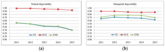
Figure 1.
Mean efficiencies of the Chinese industrial systems between 2011 and 2015: (a) Natural disposability; (b) Managerial disposability.
Although the technical inefficiency is mainly sourced from the low ENE, some regions, like Hebei (in 2015 under managerial disposability), have better pollutant control than regular production. There are great disparities in inefficiencies of period efficiency among different regions. We took Zhejiang and Liaoning as examples to further illustrate this point. It is observed that the ECEs are all lower than the ENEs in Zhejiang between 2011 and 2015. A suggestion for such regions is that they should improve their regular production first and keep the advantage of pollutant control. On the contrary, the ECEs are all greater than the ENEs in Liaoning during 2011–2015, that is Liaoning performs badly on pollutant control but well in regular production. For such regions, improvement in pollutant control is more urgent. These analytical results show the necessity and importance of decomposition of TE, thereby potentially gaining more helpful information into efficiency improvement.
Figure 2 depicts the efficiency comparisons of three areas during the study period. As visually summarized in Figure 2, the TE, ECE, and ENE of the three areas have a downward trend under natural disposability. In contrast, such trends do not occur under managerial disposability. Under natural disposability, the eastern region has the largest TE and ENE. Under managerial disposability, the western area has the lowest TE and ENE, and the central area gradually catches up with the eastern area regarding TE and ENE. This implies that increasing the capital investment for technological innovation can effectively improve the central area’s TE and ENE. The low TE and ENE of the western area may be caused by the shortage of capital investment for technological innovation, and it should implement policies to support technological innovation for clean production. The results of efficiency comparisons for the three areas are consistent with the situation of economic development in China. In China, the eastern area has the most development while the western area has the least development. The eastern area has sufficient capital investment for clean production technology. Due to its shortage of capital investment for clean technology, the western area has the worst performance in TE and ENE.
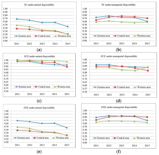
Figure 2.
Efficiency comparisons of three areas between 2011 and 2015: (a) TE under natural disposability; (b) TE under managerial disposability; (c) ECE under natural disposability; (d) ECE under managerial disposability; (e) ENE under natural disposability; (f) ENE under managerial disposability.
Note that the TEs and ENEs of the three areas under managerial disposability are all greater than those under natural disposability. This result indicates that a positive strategy (managerial disposability) is more helpful to provide the possibility for TE and ENE improvements. The regional industrial systems of the three areas should consider environmental regulation as an opportunity and take major strategic actions to utilize clean production technology. Only in this way can the regional industrial systems simultaneously achieve economic benefits and environmental protection.
3.2.2. Dynamic Efficiency Analysis
We also calculated the MPIs to examine the changes in TE, ECE, and ENE of 30 regional industrial systems over time. Table 6, Table 7 and Table 8 show the calculated results for all the consecutive two-year periods over 2011–2015.
Table 6.
The Malmqusit productivity index (MPI) values of TE for Chinese industrial systems (2011–2015).
Table 7.
The MPI values of ECE for Chinese industrial systems (2011–2015).
Table 8.
The MPI values of ENE for Chinese industrial systems (2011–2015).
It can be observed in Table 6, Table 7 and Table 8 that the average MPI values of TE, ECE, and ENE under natural disposability are all lower than those under managerial disposability. It implies that increasing the capital investment for technological innovation has a positive effect on the TE, ECE, and ENE. That is the positive strategy is more helpful in improving efficiency in the dynamic context.
In Table 6, the Chinese regional industrial systems experience positive change under managerial disposability, implying that the Chinese regional industrial systems’ TEs have been improved. However, under natural disposability, one period of time, i.e., 2014/2015, displays a negative change (i.e., below unity). The regional average MPI values of TE during the study period indicate that all the regions except Heilongjiang have an improvement in their TEs under managerial disposability. Among them, Beijing in the eastern area and Shaanxi in the western area are found to have relatively high annual growth rate.
It can be observed in Table 7 and Table 8 that the MPI values of ECE are all lower than those of ENEs under managerial disposability. This suggests that the changes in ENE are more significant than those in ECE, and the Chinese government’s environmental regulation policies have achieved remarkable effects on industrial pollution control.
Additionally, in Table 7, regarding the MPI values of ECE under managerial disposability, we find that Jiangsu in the eastern area has the highest annual growth rate. That is Jiangsu performs well in regular production activities. In Table 8, regarding the MPI values of ENE under managerial disposability, we find that Beijing in the eastern area and Ningxia in the western area have relatively high annual growth rate. That is these two regions do well on industrial pollution control.
Figure 3 displays the average MPI values of Chinese industrial systems over time. Note that the MPI values of TE and ENE have the same trend under both natural disposability and managerial disposability. This observation suggests that the TE is mainly affected by ENE in the dynamic context. In order to enhance the TE, the Chinese industrial systems should take ENE into consideration and make more efforts to improve ENE.
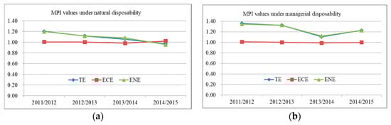
Figure 3.
Mean Malmqusit productivity index (MPI) values of Chinese industrial systems over time: (a) MPI values under natural disposability; (b) MPI values under managerial disposability.
In Figure 3, it is also found that the MPI values of TE and ENE are all greater than those of ECE under managerial disposability. This observation verifies that the TE and ENE can be improved significantly under managerial disposability and the decision makers should guarantee capital investment for technological innovation.
The above-mentioned efficiency differences between natural disposability and managerial disposability are confirmed graphically by Figure 4. As shown in Figure 4, the average MPI values of TE and ENE under managerial disposability are all greater than those under natural disposability. All these observations suggest that increasing the capital investment for technological innovation has a positive effect on the TE and ENE. Therefore, in the following discussions, we focus on the analysis of efficiency changes under managerial disposability.
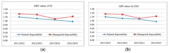
Figure 4.
Mean MPI values of TE and ENE over time: (a) MPE values of TE; (b) MPI values for ENE.
We further decomposed the MPI values of TE and ENE into the effects of static efficiency change and (EC) technical change (TC) using Equations (20) and (22) in order to identify the driving factors of TE and ENE changes. Table 9 reports the EC and TC values of TE. (For the EC and TC values of ENE, see Appendix B.)
Table 9.
The EC and TC values of TE for Chinese industrial systems (2011–2015).
In Table 9, the third to sixth columns report the static efficiency changes of TE. The seventh to tenth columns describe the technical changes of TE. Analysis of Table 9 yields the following:
- (1)
- With regard to the static efficiency change, we find that 30 regions as a whole have a rise in their efficiency change scores over time. Furthermore, Beijing, Tianjin, Jiangsu, Jilin, Jiangxi, and Inner Mongolia do not experience changes in their TEs (i.e., ) over time, which means that they are always on the production frontier. Among 30 regions, 13 regions show a decrease in annual change score; this suggests that these regions are not successful in catching up with the frontier.
- (2)
- Regarding the technical change, it is found that all 30 regions show technical improvement during the study period. This means that the regional industrial systems all perform well in promoting technological progress.
- (3)
- The scores of the technical change are all higher than those of the static efficiency change. It means that the MPI value of TE is mainly constituted by the technical change.
Figure 5 shows the average static efficiency change and technical change values of TE and ENE. In Figure 5, we find that the static efficiency change and technical change of TE are identical to those of ENE. Specifically, the MPI values of TE and ENE are mainly affected by the technical changes. Furthermore, the average EC values are close to unity (e.g., in Figure 5a, the minimum is 0.9191 and the maximum is 1.1090), and the average TC values are all greater than unity (e.g., in Figure 5b, the minimum is 1.1249 and the maximum is 1.3634). It may be concluded that the TE have not experienced remarkable change and the catching-up effect is not distinct, and also the Chinese regional industrial systems have experienced a significant technical improvement. All these observations suggest that the improvement in Chinese industrial efficiency may be mainly attributed to technical improvement rather than the static efficiency change.
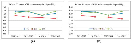
Figure 5.
Mean EC and TC values of Chinese industrial systems over time: (a) EC and TC values of TE under managerial disposability; (b) EC and TC values of ENE under managerial disposability.
The above-mentioned findings are consistent with the situation in Chinese industry. Since the reform and opening-up, Chinese industry has been committed to technological innovation and industrial technology has reached a new level. For example, from 2004 to 2016, the research and development (R&D) companies, R&D personnel and R&D expenditures increased by 4.1 times, 3.5 times, and 8.9 times respectively. On other hand, from 2004 to 2016, the sales revenue of new industrial products increased by 6.7 times, with an average annual growth rate of 18.5%. The continuous technological progress of industrial enterprises has become an important force in driving China’s innovation. The global innovation index released by the World Intellectual Property Organization (WIPO) shows that the comprehensive ranking of China’s innovation capability has risen from 34th in 2012 to 22nd in 2017.
4. Conclusions
This study proposes static and dynamic DEA models to evaluate the technical efficiencies of industrial systems. The operational process of an industrial system is characterized as implementing two types of activities, i.e., regular production activities and pollutant control activities. The duties of the former activities are to generate desirable outputs for economic benefit, while the missions of the latter activities are to reduce undesirable outputs for sustainable development. We decomposed technical efficiency into economic efficiency and environmental efficiency to portray the performance of the two types of activities. Based on the proposed model, the TE, ECE, ENE, and MPI values are obtained simultaneously. The dynamic efficiency changes were also divided into two components (i.e., static efficiency change and technical change) to explore what drives the changes in TE over time. Since the proposed models decompose TE into ECE and ENE and analyze dynamic efficiency changes, they have a higher discriminating power for the sources of inefficiencies in industrial systems than the existing DEA models.
The proposed approach was applied to examine the technical efficiencies of Chinese regional industrial systems between 2011 and 2015. The major findings are summarized as follows. First, the low ENE is the main source of technical inefficiency. Second, the average static TEs and ENEs under natural disposability are all lower than those under managerial disposability. This finding indicates that a regional industrial system can improve its TE and ENE by increasing the capital investment for technological innovation. Third, the MPI values of TE and ENE have the same trend, and the static efficiency change and technical change of TE are identical to those of ENE. This finding further verifies that the TE is mainly affected by the ENE. Finally, the static efficiency change has an insignificant impact while the technical change has a significant impact on the changes in TE. It means that the TE improvement in the Chinese industrial system is mainly driven by technical improvement, especially the technical improvement of pollutant control.
Based on the above findings, we supply the following policy implications for the sustainable development of regional industrial systems in China. (1) More effort should be exerted to enhance the ENE. It is recommended that the Chinese government takes comprehensive measures to fully mobilize the initiative of industrial enterprises for enhancing the ENE, such as improving the laws and regulations on environmental protection, implementing green credit policy, and promoting environmental tax policy. (2) Increasing capital investment for technological innovation. The Chinese government should provide appropriate financial support for industrial enterprises to promote technological innovation, e.g., arranging the ring-fenced funding, developing technology finance, and granting financial subsidies. (3) Encouraging industrial enterprises to improve the level of clean technology. It is suggested that the Chinese government establishes an incentive mechanism to fully mobilize the initiative of industrial enterprises for technological innovation, for example, encouraging industrial enterprises to establish innovative teams, cooperate with universities, undertake major technological innovation projects, and transform scientific and technological achievements.
In this study, we considered the two types of activities of industrial systems. Actually, the operational process of an industrial system is composed of many activities, such as, two-stage process or network structure. Further research may be conducted by exploring the internal structure of industrial systems by using the network DEA approach. In addition, we only estimated the technical efficiencies of Chinese regional industrial systems between 2011 and 2015, and thus a longer time period would be a useful extension to our study.
Author Contributions
Conceptualization, L.Z. (Linlin Zhao); methodology, L.Z. (Linlin Zhao) and L.Z. (Lin Zhang); writing—original draft preparation, L.Z. (Linlin Zhao); writing—review & editing, L.Z. (Lin Zhang) and Y.Z.; funding acquisition, L.Z. (Linlin Zhao) and Y.Z.
Funding
This work was supported by the National Natural Science Foundation of China (Grant nos. 71701102, 71701111, and 71671173) and the Philosophy and Social Science Foundation of Jiangsu Higher Education Institutions of China (Grant no. 2018SJA0326).
Conflicts of Interest
The authors declare no conflict of interest.
Appendix A
The process of model transformation.
Let , then model (4) becomes:
Nevertheless, model (A1) is still a nonlinear programming since it contains the nonlinear terms in the objective function and in the constraints. Let
Then model (A1) can be transformed into the following linear form:
By solving model (A2), we can obtain the optimal solution and the TE. Using Equation (A2), and can be obtained. Further applying Equations (5) and (6), we can then calculate ECE and ENE.
Similar to model (4), model (8) can be transformed into the following linear form:
Similar to model (4), model (13) can be transformed into the following linear form:
Similar to model (4), model (18) can be transformed into the following linear form:
Appendix B
Detail results of EC and TC for ENE.
Table A1.
The EC and TC values of ENE for Chinese industrial systems (2011–2015).
Table A1.
The EC and TC values of ENE for Chinese industrial systems (2011–2015).
| Areas | |||||||||
|---|---|---|---|---|---|---|---|---|---|
| 2011/2012 | 2012/2013 | 2013/2014 | 2014/2015 | 2011/2012 | 2012/2013 | 2013/2014 | 2014/2015 | ||
| Eastern area | Beijing | 1.0000 | 1.0000 | 1.0000 | 1.0000 | 0.8960 | 2.8669 | 0.5059 | 1.9765 |
| Tianjin | 1.0000 | 1.0000 | 1.0000 | 1.0000 | 1.2318 | 1.2773 | 1.0000 | 1.0000 | |
| Hebei | 1.2427 | 1.1178 | 1.1245 | 1.1111 | 1.0966 | 1.1243 | 1.3072 | 1.3486 | |
| Liaoning | 1.2458 | 1.0613 | 0.8432 | 0.4680 | 1.0308 | 1.2285 | 1.0632 | 1.5453 | |
| Shanghai | 0.9112 | 0.8952 | 0.7813 | 0.7354 | 1.2691 | 1.1017 | 1.2881 | 1.9174 | |
| Jiangsu | 1.0000 | 1.0000 | 1.0000 | 1.0000 | 1.2724 | 1.3045 | 1.0846 | 1.0922 | |
| Zhejiang | 1.1481 | 1.0599 | 0.9180 | 0.8225 | 1.1330 | 1.1114 | 1.3102 | 1.4714 | |
| Fujian | 1.0282 | 1.0497 | 0.9668 | 1.0159 | 1.2862 | 1.3116 | 1.0625 | 1.2621 | |
| Shandong | 1.2234 | 0.9553 | 1.1205 | 0.8032 | 1.0175 | 1.3269 | 1.0014 | 1.6036 | |
| Guangdong | 1.1067 | 1.1206 | 0.8789 | 0.7858 | 1.0604 | 1.0955 | 1.3714 | 1.7742 | |
| Hainan | 1.0672 | 0.5912 | 1.4551 | 0.4319 | 1.2310 | 0.9069 | 1.3283 | 0.8431 | |
| Mean | 1.0885 | 0.9864 | 1.0080 | 0.8340 | 1.1386 | 1.3323 | 1.1203 | 1.4395 | |
| Central area | Jilin | 1.0000 | 1.0000 | 1.0000 | 1.0000 | 1.8808 | 1.2375 | 1.1613 | 1.0000 |
| Heilongjiang | 0.8961 | 1.0715 | 0.7161 | 0.7835 | 1.1278 | 1.0637 | 0.8631 | 1.6757 | |
| Shanxi | 1.1596 | 1.0577 | 1.0170 | 1.0112 | 1.0371 | 1.2827 | 0.9555 | 1.6775 | |
| Anhui | 1.1596 | 1.0577 | 1.0170 | 1.0112 | 1.2808 | 1.2371 | 1.0475 | 1.4158 | |
| Jiangxi | 1.0000 | 1.0000 | 1.0000 | 1.0000 | 1.4783 | 1.3749 | 1.1208 | 1.0000 | |
| Henan | 1.3089 | 1.0503 | 1.1080 | 0.9143 | 1.0663 | 1.2434 | 1.1299 | 1.3946 | |
| Hubei | 1.3042 | 1.0000 | 1.0000 | 1.0000 | 1.0899 | 1.3494 | 1.0782 | 1.3100 | |
| Hunan | 1.3526 | 1.1139 | 1.0142 | 1.0000 | 1.0348 | 1.2955 | 1.1414 | 1.3817 | |
| Mean | 1.1630 | 1.0304 | 0.9923 | 0.9277 | 1.2495 | 1.2605 | 1.0622 | 1.3569 | |
| Western area | Inner Mongolia | 1.0000 | 1.0000 | 1.0000 | 1.0000 | 1.1645 | 1.0000 | 1.0000 | 0.9118 |
| Guangxi | 1.3334 | 1.1564 | 1.0701 | 1.0247 | 1.0445 | 1.1110 | 1.3207 | 1.3498 | |
| Chongqing | 1.0000 | 0.6307 | 1.0919 | 1.2390 | 1.2920 | 2.0310 | 1.1253 | 1.3646 | |
| Sichuan | 1.2246 | 0.9812 | 0.9138 | 0.7111 | 1.0234 | 1.2077 | 1.0782 | 1.6258 | |
| Guizhou | 1.0641 | 0.9798 | 1.0815 | 0.7934 | 1.0108 | 1.1961 | 1.0664 | 1.6249 | |
| Yunnan | 1.0709 | 1.0931 | 0.9778 | 0.9581 | 1.2054 | 1.1684 | 1.1823 | 1.4377 | |
| Shaanxi | 1.0000 | 1.0000 | 1.0000 | 0.4709 | 3.0772 | 1.3619 | 0.7401 | 1.3511 | |
| Gansu | 1.1385 | 1.5493 | 0.7963 | 0.7064 | 1.4174 | 1.0721 | 1.3667 | 1.2470 | |
| Qinghai | 0.9014 | 1.2148 | 0.9425 | 1.0610 | 0.8909 | 1.3388 | 1.4117 | 1.0846 | |
| Ningxia | 0.9135 | 1.3489 | 1.1402 | 1.2738 | 1.5357 | 1.1618 | 1.1792 | 1.3763 | |
| Xinjiang | 1.1139 | 0.7447 | 0.9653 | 1.3910 | 0.8147 | 1.9647 | 1.4838 | 1.0559 | |
| Mean | 1.0691 | 1.0635 | 0.9981 | 0.9663 | 1.3161 | 1.3285 | 1.1777 | 1.3118 | |
| China | Mean | 1.1069 | 1.0268 | 0.9995 | 0.9093 | 1.2347 | 1.3071 | 1.1201 | 1.3694 |
References
- Sueyoshi, T.; Goto, M. Data envelopment analysis for environmental assessment: Comparison between public and private ownership in petroleum industry. Eur. J. Oper. Res. 2012, 216, 668–678. [Google Scholar] [CrossRef]
- Wu, F.; Fan, L.W.; Zhou, P.; Zhou, D.Q. Industrial energy efficiency with CO2 emissions in China: A nonparametric analysis. Energy Policy 2012, 49, 164–172. [Google Scholar] [CrossRef]
- Chen, L.; Jia, G. Environmental efficiency analysis of China’s regional industry: A data envelopment analysis (DEA) based approach. J. Clean. Prod. 2017, 142, 846–853. [Google Scholar] [CrossRef]
- Wang, K.; Wei, Y.M. China’s regional industrial energy efficiency and carbon emissions abatement costs. Appl. Energy 2014, 130, 617–631. [Google Scholar] [CrossRef]
- Zhang, B.; Bi, J.; Fan, Z.; Yuan, Z.; Ge, J. Eco-efficiency analysis of industrial system in China: A data envelopment analysis approach. Ecol. Econ. 2008, 68, 306–316. [Google Scholar] [CrossRef]
- Meng, F.; Su, B.; Thomson, E.; Zhou, D.; Zhou, P. Measuring China’s regional energy and carbon emission efficiency with DEA models: A survey. Appl. Energy 2016, 183, 1–21. [Google Scholar] [CrossRef]
- Emrouznejad, A.; Yang, G.L. CO2 emissions reduction of Chinese light manufacturing industries: A novel RAM-based global Malmquist-Luenberger productivity index. Energy Policy 2016, 96, 397–410. [Google Scholar] [CrossRef]
- Zhao, L.; Zha, Y.; Liang, N.; Liang, L. Data envelopment analysis for unified efficiency evaluation: An assessment of regional industries in China. J. Clean. Prod. 2016, 113, 695–704. [Google Scholar] [CrossRef]
- Kao, C.; Hwang, S.N. Multi-period efficiency and Malmquist productivity index in two-stage production systems. Eur. J. Oper. Res. 2014, 232, 512–521. [Google Scholar] [CrossRef]
- Färe, R.; Grosskopf, S. Productivity and intermediate products: A frontier approach. Econ. Lett. 1996, 50, 65–70. [Google Scholar] [CrossRef]
- Zhou, H.; Yang, Y.; Chen, Y.; Zhu, J. Data envelopment analysis application in sustainability: The origins, development and future directions. Eur. J. Oper. Res. 2018, 264, 1–16. [Google Scholar] [CrossRef]
- Yang, C.C. An enhanced DEA model for decomposition of technical efficiency in banking. Ann. Oper. Res. 2014, 214, 167–185. [Google Scholar] [CrossRef]
- Zha, Y.; Liang, N.; Wu, M.; Bian, Y. Efficiency evaluation of banks in China: A dynamic two-stage slacks-based measure approach. Omega 2016, 60, 60–72. [Google Scholar] [CrossRef]
- Arcos-Vargas, A.; Núñez-Hernández, F.; Villa-Caro, G. A DEA analysis of electricity distribution in Spain: An industrial policy recommendation. Energy Policy 2017, 102, 583–592. [Google Scholar] [CrossRef]
- Makridou, G.; Andriosopoulos, K.; Doumpos, M.; Zopounidis, C. Measuring the efficiency of energy-intensive industries across European countries. Energy Policy 2016, 88, 573–583. [Google Scholar] [CrossRef]
- Goto, M.; Otsuka, A.; Sueyoshi, T. DEA (Data Envelopment Analysis) assessment of operational and environmental efficiencies on Japanese regional industries. Energy 2014, 66, 535–549. [Google Scholar] [CrossRef]
- Wang, D.; Li, S.; Sueyoshi, T. DEA environmental assessment on US Industrial sectors: Investment for improvement in operational and environmental performance to attain corporate sustainability. Energy Econ. 2014, 45, 254–267. [Google Scholar] [CrossRef]
- Bian, Y.; Liang, N.; Xu, H. Efficiency evaluation of Chinese regional industrial systems with undesirable factors using a two-stage slacks-based measure approach. J. Clean. Prod. 2015, 87, 348–356. [Google Scholar] [CrossRef]
- Chen, L.; Lai, F.; Wang, Y.M.; Huang, Y.; Wu, F.M. A two-stage network data envelopment analysis approach for measuring and decomposing environmental efficiency. Comput. Ind. Eng. 2018, 119, 388–403. [Google Scholar] [CrossRef]
- Liu, Y.; Wang, K. Energy efficiency of China’s industry sector: An adjusted network DEA (data envelopment analysis)-based decomposition analysis. Energy 2015, 93, 1328–1337. [Google Scholar] [CrossRef]
- Wu, J.; Zhu, Q.; Ji, X.; Chu, J.; Liang, L. Two-stage network processes with shared resources and resources recovered from undesirable outputs. Eur. J. Oper. Res. 2016, 251, 182–197. [Google Scholar] [CrossRef]
- Wu, J.; Xiong, B.; An, Q.; Sun, J.; Wu, H. Total-factor energy efficiency evaluation of Chinese industry by using two-stage DEA model with shared inputs. Ann. Oper. Res. 2017, 255, 257–276. [Google Scholar] [CrossRef]
- Halkos, G.E.; Tzeremes, N.G.; Kourtzidis, S.A. Measuring sustainability efficiency using a two-stage data envelopment analysis approach. J. Ind. Ecol. 2016, 20, 1159–1175. [Google Scholar] [CrossRef]
- Li, Y.; Shi, X.; Emrouznejad, A.; Liang, L. Environmental performance evaluation of Chinese industrial systems: A network SBM approach. J. Oper. Res. Soc. 2018, 69, 825–839. [Google Scholar] [CrossRef]
- Fernández, D.; Pozo, C.; Folgado, R.; Jiménez, L.; Guillén-Gosálbez, G. Productivity and energy efficiency assessment of existing industrial gases facilities via data envelopment analysis and the Malmquist index. Appl. Energy 2018, 212, 1563–1577. [Google Scholar] [CrossRef]
- Sueyoshi, T.; Goto, M.; Sugiyama, M. DEA window analysis for environmental assessment in a dynamic time shift: Performance assessment of US coal-fired power plants. Energy Econ. 2013, 40, 845–857. [Google Scholar] [CrossRef]
- Zhang, N.; Wang, B.; Liu, Z. Carbon emissions dynamics, efficiency gains, and technological innovation in China’s industrial sectors. Energy 2016, 99, 10–19. [Google Scholar] [CrossRef]
- Zhang, R.; Lu, C.C.; Lee, J.H.; Feng, Y.; Chiu, Y.H. Dynamic Environmental Efficiency Assessment of Industrial Water Pollution. Sustainability 2019, 11, 3053. [Google Scholar] [CrossRef]
- Chen, S.; Golley, J. ‘Green’ productivity growth in China’s industrial economy. Energy Econ. 2014, 44, 89–98. [Google Scholar] [CrossRef]
- Yao, X.; Guo, C.; Shao, S.; Jiang, Z. Total-factor CO2 emission performance of China’s provincial industrial sector: A meta-frontier non-radial Malmquist index approach. Appl. Energy 2016, 184, 1142–1153. [Google Scholar] [CrossRef]
- Charnes, A.; Cooper, W.W. Programming with linear fractional functions. Nav. Res. Logist. Q. 1962, 9, 181–186. [Google Scholar] [CrossRef]
- Tone, K. A slacks-based measure of efficiency in data envelopment analysis. Eur. J. Oper. Res. 2011, 130, 498–509. [Google Scholar] [CrossRef]
- Caves, D.W.; Christensen, L.R.; Diewert, W.E. The economic theory of index numbers and the measurement of input, output, and productivity. Econometrica 1982, 50, 1393–1414. [Google Scholar] [CrossRef]
- Färe, R.; Grosskopf, S.; Norris, M.; Zhang, Z. Productivity growth, technical progress, and efficiency change in industrialized countries. Am. Econ. Rev. 1994, 84, 66–83. [Google Scholar]
- Pastor, J.T.; Lovell, C.K. A global Malmquist productivity index. Econ. Lett. 2005, 88, 266–271. [Google Scholar] [CrossRef]
© 2019 by the authors. Licensee MDPI, Basel, Switzerland. This article is an open access article distributed under the terms and conditions of the Creative Commons Attribution (CC BY) license (http://creativecommons.org/licenses/by/4.0/).