A New Trend in the Space–Time Distribution of Cultivated Land Occupation for Construction in China and the Impact of Population Urbanization


Abstract
:1. Introduction
2. Materials and Methods
2.1. Materials
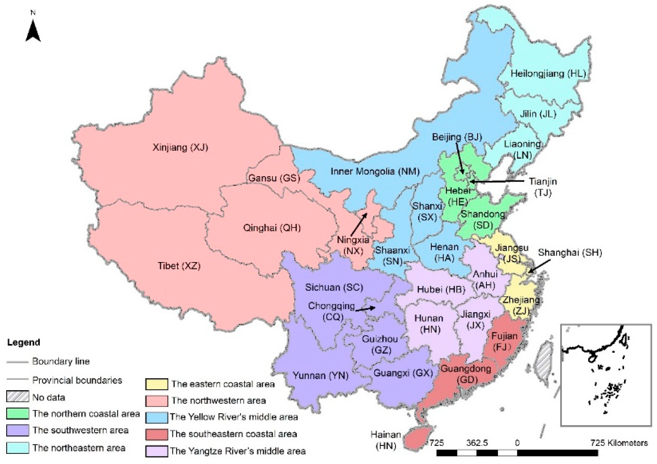
2.1.1. Study Area
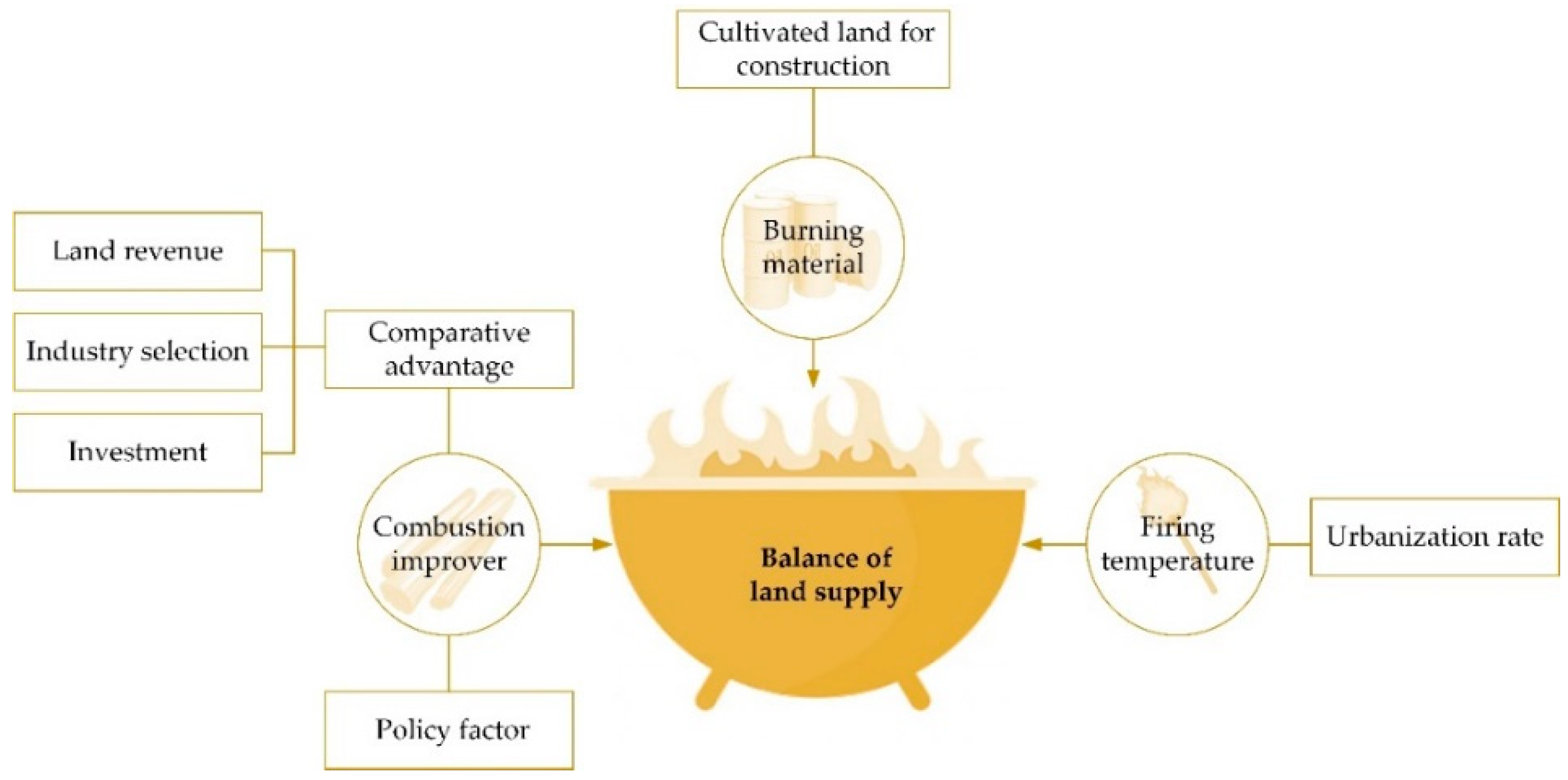
2.1.2. An Analysis Framework of the Driving Factors of Cultivated Land Occupation for Construction (CLOC)
2.1.3. Data Source and Processing
2.2. Methods (Geode (1.12) and ArcMap (10.5) Software Were Used in ESDA (Including Outlier Analysis, Global and Local Spatial Autocorrelation), and the Spatial Regression Analysis Was Performed by MATLAB (R2016a) Software)
2.2.1. Global Spatial Autocorrelation
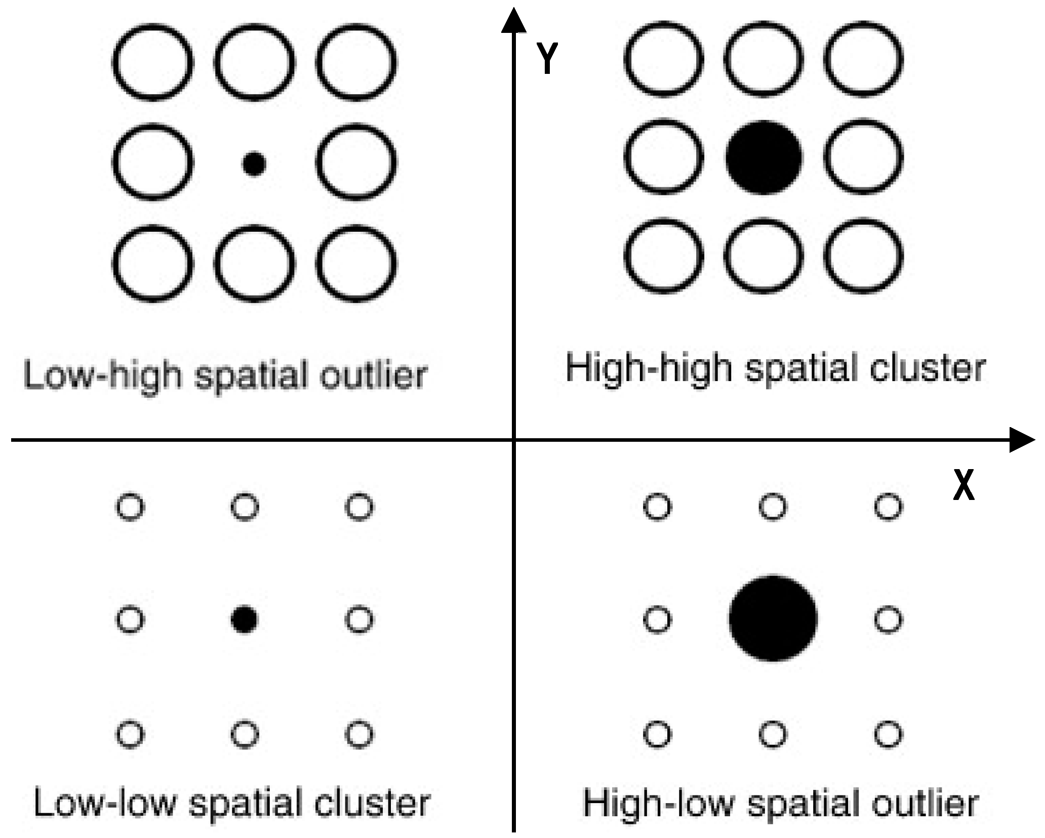
2.2.2. Local Spatial Autocorrelation
2.2.3. The Spatial Weight Matrix
2.2.4. Spatial Econometrics Models
3. Results
3.1. Exploratory Spatial Data Analysis of CLOC
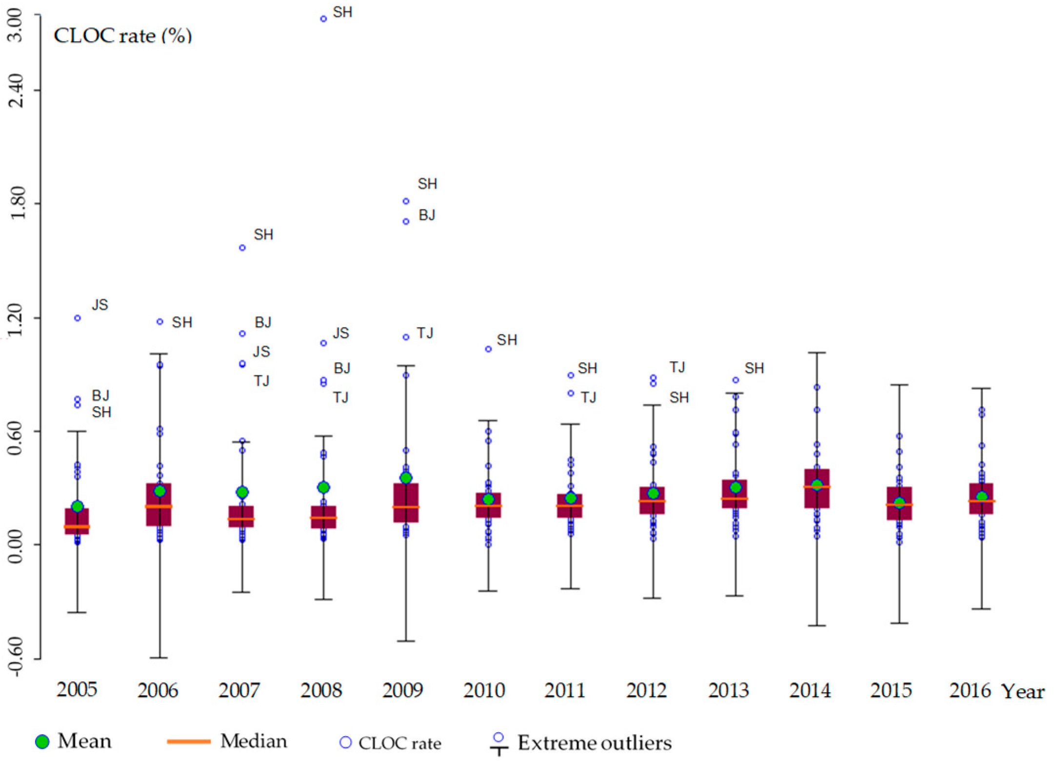
3.1.1. Outlier Analysis
3.1.2. Global Association
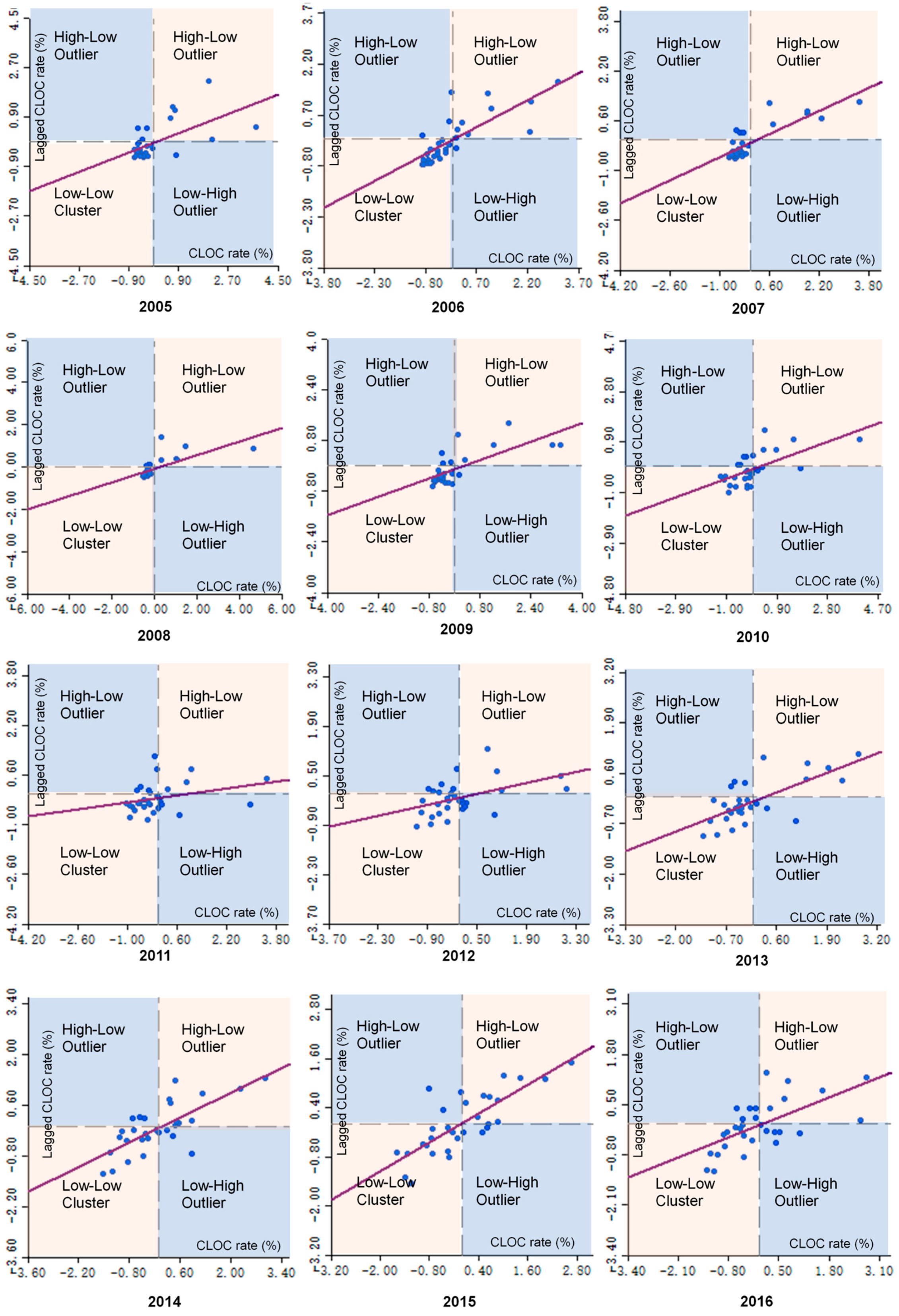
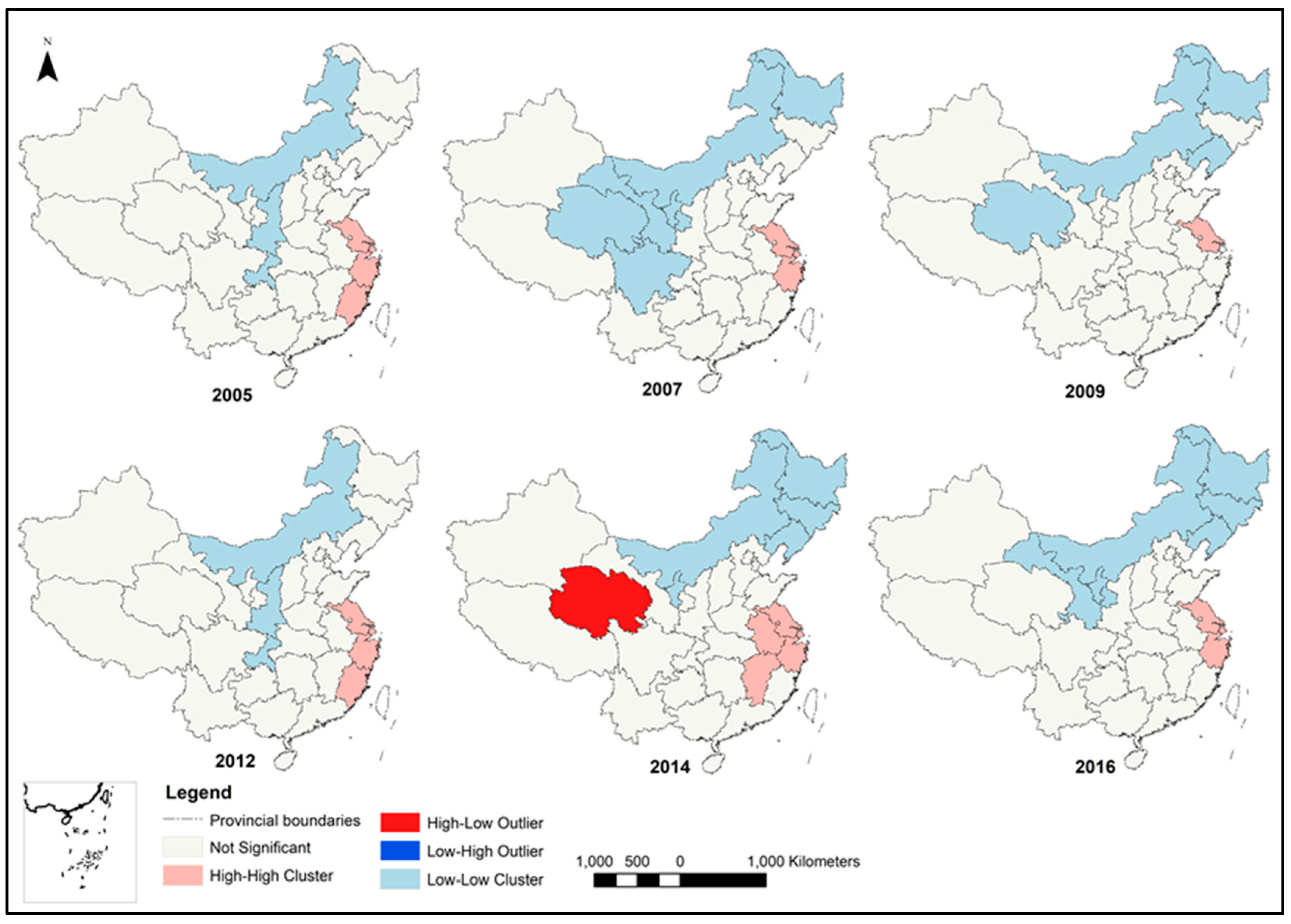
3.1.3. Local Association
3.2. The Driving Force Analysis
3.2.1. The Non-Spatial Regression Model Analysis
3.2.2. The Spatial Durbin Regression Model Analysis
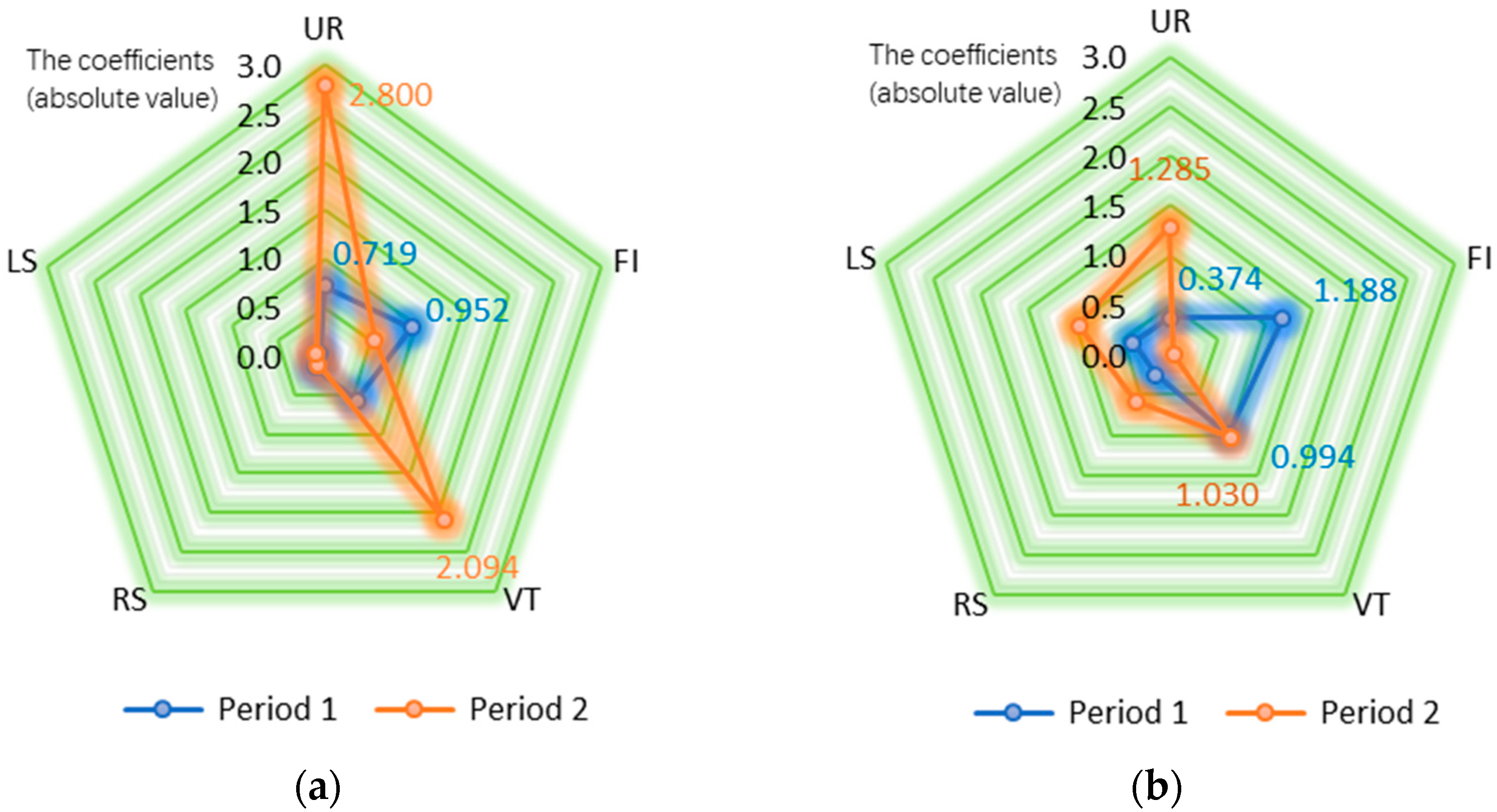
3.2.3. The Changes in the Driving Factors in Two Periods
4. Discussion
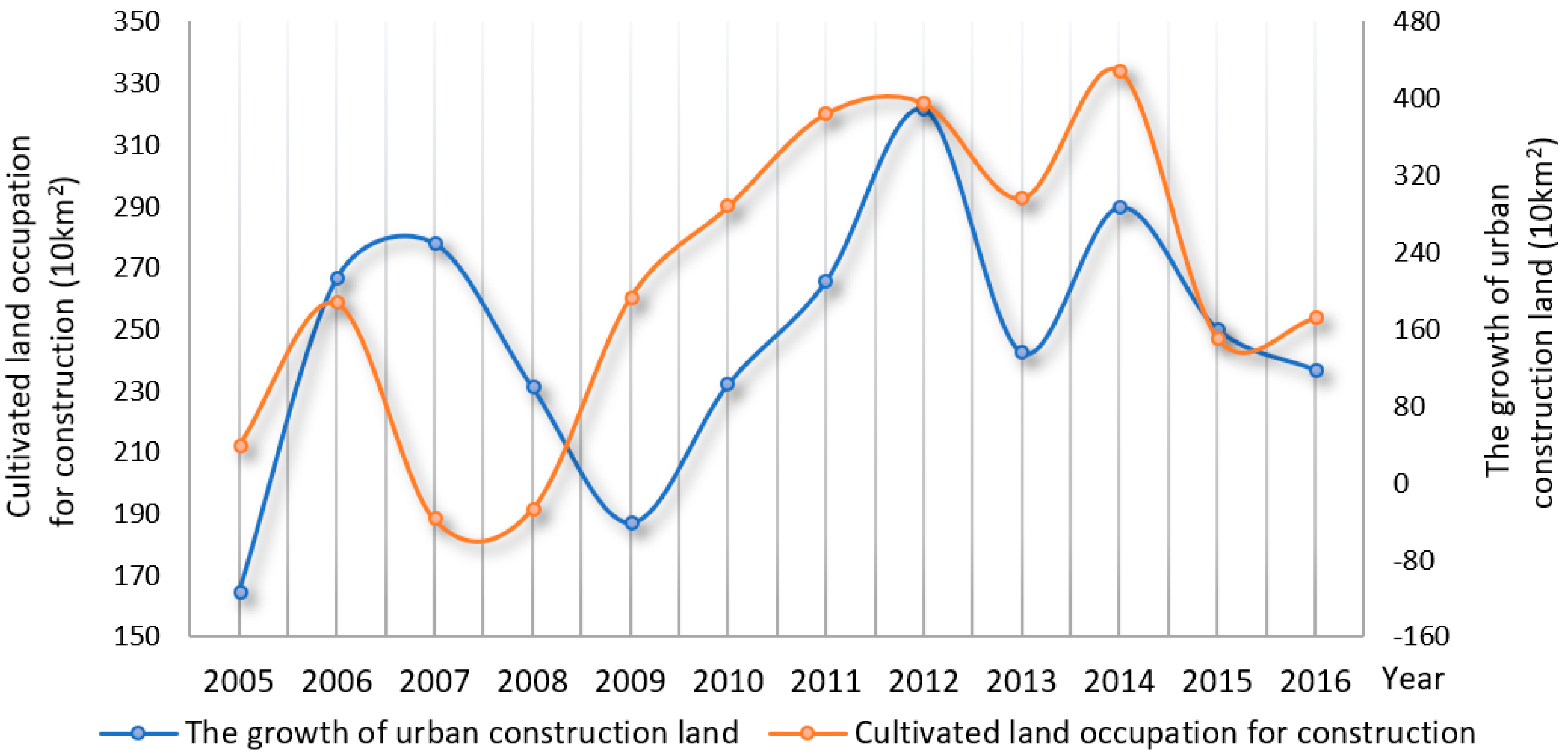
4.1. Characteristics of Time and Space Distribution of CLOC
4.2. The Impact of Population Urbanization and Other Driving Factors
4.3. Policy Recommendations
5. Conclusions
Author Contributions
Funding
Acknowledgments
Conflicts of Interest
References
- Haberl, H. Competition for land: A sociometabolic perspective. Ecol. Econ. 2015, 119, 424–431. [Google Scholar] [CrossRef] [Green Version]
- Li, Y.; Wu, W.; Liu, Y. Land consolidation for rural sustainability in China: Practical reflections and policy implications. Land Use Policy 2018, 74, 137–141. [Google Scholar] [CrossRef]
- Liu, T.; Liu, H.; Qi, Y. Construction land expansion and cultivated land protection in urbanizing China: Insights from national land surveys, 1996–2006. Habitat Int. 2015, 46, 13–22. [Google Scholar] [CrossRef]
- You, H.; Yang, X. Urban expansion in 30 megacities of China: Categorizing the driving force profiles to inform the urbanization policy. Land Use Policy 2017, 68, 531–551. [Google Scholar] [CrossRef]
- Long, H.; Ge, D.; Zhang, Y.; Tu, S.; Qu, Y.; Ma, L. Changing man-land interrelations in China’s farming area under urbanization and its implications for food security. J. Environ. Manag. 2018, 209, 440–451. [Google Scholar] [CrossRef] [PubMed]
- Shao, Z.; Bakker, M.; Spit, T.; Janssen-Jansen, L.; Qun, W. Containing urban expansion in China: The case of Nanjing. J. Environ. Plan. Manag. 2019, 62, 1–21. [Google Scholar] [CrossRef]
- Chen, J.; Gao, J.; Chen, W. Urban land expansion and the transitional mechanisms in Nanjing, China. Habitat Int. 2016, 53, 274–283. [Google Scholar] [CrossRef]
- Song, W.; Deng, X. Effects of urbanization-induced cultivated land loss on ecosystem services in the North China Plain. Energies 2015, 8, 5678–5693. [Google Scholar] [CrossRef]
- Song, W. Decoupling cultivated land loss by construction occupation from economic growth in Beijing. Habitat Int. 2014, 43, 198–205. [Google Scholar] [CrossRef]
- Liu, Y.; Yang, Y.; Li, Y.; Li, J. Conversion from rural settlements and arable land under rapid urbanization in Beijing during 1985–2010. J. Rural Stud. 2017, 51, 141–150. [Google Scholar] [CrossRef]
- Deng, X.; Gibson, J.; Wang, P. Management of trade-offs between cultivated land conversions and land productivity in Shandong Province. J. Clean. Prod. 2017, 142, 767–774. [Google Scholar] [CrossRef]
- Luo, T.; Tan, R.; Kong, X.; Zhou, J. Analysis of the Driving Forces of Urban Expansion Based on a Modified Logistic Regression Model: A Case Study of Wuhan City, Central China. Sustainability 2019, 11, 2207. [Google Scholar] [CrossRef]
- Wang, J.; He, T.; Lin, Y. Changes in ecological, agricultural, and urban land space in 1984–2012 in China: Land policies and regional social-economical drivers. Habitat Int. 2018, 71, 1–13. [Google Scholar] [CrossRef]
- Zhang, W.; Wang, M.Y. Spatial-temporal characteristics and determinants of land urbanization quality in China: Evidence from 285 prefecture-level cities. Sustain. Cities Soc. 2018, 38, 70–79. [Google Scholar] [CrossRef]
- Liu, J.Y.; Zhan, J.Y.; Deng, X.Z. Spatio-temporal patterns and driving forces of urban land expansion in China during the economic reform era. AMBIO 2005, 34, 450–455. [Google Scholar] [CrossRef] [PubMed]
- Liu, Y.; Wang, L.; Long, H. Spatio-temporal analysis of land-use conversion in the eastern coastal China during 1996–2005. J. Geogr. Sci. 2008, 18, 274–282. [Google Scholar] [CrossRef]
- Li, X.; Zhou, W.; Ouyang, Z. Forty years of urban expansion in Beijing: What is the relative importance of physical, socioeconomic, and neighborhood factors? Appl. Geogr. 2013, 38, 1–10. [Google Scholar] [CrossRef]
- Li, G.; Sun, S.; Fang, C. The varying driving forces of urban expansion in China: Insights from a spatial-temporal analysis. Landsc. Urban Plan. 2018, 174, 63–77. [Google Scholar] [CrossRef]
- Zhang, L.; Lu, D.; Li, Q.; Lu, S. Impacts of socioeconomic factors on cropland transition and its adaptation in Beijing, China. Environ. Earth Sci. 2018, 77, 575. [Google Scholar] [CrossRef]
- Lang, W.; Long, Y.; Chen, T. Rediscovering Chinese cities through the lens of land-use patterns. Land Use Policy 2018, 79, 362–374. [Google Scholar] [CrossRef]
- Xia, C.; Zhang, A.; Wang, H.; Zhang, B.; Zhang, Y. Bidirectional urban flows in rapidly urbanizing metropolitan areas and their macro and micro impacts on urban growth: A case study of the Yangtze River middle reaches megalopolis, China. Land Use Policy 2019, 82, 158–168. [Google Scholar] [CrossRef]
- Wang, K.; Qi, W. Space-time relationship between urban municipal district adjustment and built-up area expansion in China. Chin. Geogr. Sci. 2017, 27, 165–175. [Google Scholar] [CrossRef]
- Li, Y.; Chen, C.; Wang, Y.; Liu, Y. Urban-rural transformation and farmland conversion in China: The application of the environmental Kuznets Curve. J. Rural Stud. 2014, 36, 311–317. [Google Scholar] [CrossRef]
- Tan, Y.; Xu, H.; Zhang, X. Sustainable urbanization in China: A comprehensive literature review. Cities 2016, 55, 82–93. [Google Scholar] [CrossRef]
- Yang, K.; Chen, B.; Du, H.; Tang, X. The contribution of cultivated land occupation by construction to China’s economic growth. J. Geogr. Sci. 2011, 21, 897–908. [Google Scholar] [CrossRef]
- Song, W.; Pijanowski, B.C. The effects of China’s cultivated land balance program on potential land productivity at a national scale. Appl. Geogr. 2014, 46, 158–170. [Google Scholar] [CrossRef]
- Niu, W.Y.; Lu, J.J.; Khan, A.A. Spatial Systems Approach to Sustainable Development: A Conceptual Framework. Environ. Manag. 1993, 17, 179–186. [Google Scholar] [CrossRef]
- Niu, W.Y.; Harris, W.M. China: The forecast of its environmental situation in the 21st century. J. Environ. Manag. 1996, 47, 101–114. [Google Scholar] [CrossRef]
- Deng, X.; Huang, J.; Rozelle, S.; Zhang, J.; Li, Z. Impact of urbanization on cultivated land changes in China. Land Use Policy 2015, 45, 1–7. [Google Scholar] [CrossRef]
- Du, X.; Huang, Z. Ecological and environmental effects of land use change in rapid urbanization: The case of hangzhou, China. Ecol. Indic. 2017, 81, 243–251. [Google Scholar] [CrossRef]
- Li, K.; Ma, Z.; Zhang, G. Evaluation of the Supply-Side Efficiency of China’s Real Estate Market: A Data Envelopment Analysis. Sustainability 2019, 11, 288. [Google Scholar] [CrossRef]
- Yoo, S.; Wagner, J.E. A review of the hedonic literatures in environmental amenities from open space: A traditional econometric vs. spatial econometric model. Int. J. Urban Sci. 2016, 20, 141–166. [Google Scholar] [CrossRef]
- Wang, Y. The Challenges and Strategies of Food Security under Rapid Urbanization in China. Sustainability 2019, 11, 542. [Google Scholar] [CrossRef]
- Pandey, B.; Seto, K.C. Urbanization and agricultural land loss in India: Comparing satellite estimates with census data. J. Environ. Manag. 2015, 148, 53–66. [Google Scholar] [CrossRef] [PubMed]
- Liang, Y.; Cai, W.; Ma, M. Carbon dioxide intensity and income level in the Chinese megacities’ residential building sector: Decomposition and decoupling analyses. Sci. Total Environ. 2019, 677, 315–327. [Google Scholar] [CrossRef] [PubMed]
- You, K.; Solomon, O.H. China’s outward foreign direct investment and domestic investment: An industrial level analysis. China Econ. Rev. 2015, 34, 249–260. [Google Scholar] [CrossRef]
- Pearson, L.J.; Pearson, L.; Pearson, C.J. Sustainable urban agriculture: Stocktake and opportunities. Int. J. Agric. Sustain. 2010, 8, 7–19. [Google Scholar] [CrossRef]
- Bengston, D.N.; Fletcher, J.O.; Nelson, K.C. Public policies for managing urban growth and protecting open space: Policy instruments and lessons learned in the United States. Landsc. Urban Plan. 2004, 69, 271–286. [Google Scholar] [CrossRef]
- Newman, L.; Powell, L.J.; Wittman, H. Landscapes of food production in agriburbia: Farmland protection and local food movements in British Columbia. J. Rural Stud. 2015, 39, 99–110. [Google Scholar] [CrossRef]
- Anselin, L.; Sridharan, S.; Gholston, S. Using exploratory spatial data analysis to leverage social indicator databases: The discovery of interesting patterns. Soc. Indic. Res. 2007, 82, 287–309. [Google Scholar] [CrossRef]
- Anselin, L. Local indicators of spatial association—LISA. Geogr. Anal. 1995, 27, 93–115. [Google Scholar] [CrossRef]
- Zhang, C.; Luo, L.; Xu, W.; Ledwith, V. Use of local Moran’s I and GIS to identify pollution hotspots of Pb in urban soils of Galway, Ireland. Sci. Total Environ. 2008, 398, 212–221. [Google Scholar] [CrossRef] [PubMed]
- Leenders, R. Modeling social influence through network autocorrelation: Constructing the weight matrix. Soc. Netw. 2002, 24, 21–47. [Google Scholar] [CrossRef]
- Laguna, F.; Eugenia Grillet, M.; Leon, J.R.; Ludena, C. Modelling malaria incidence by an autoregressive distributed lag model with spatial component. Spat. Spatio Temporal Epidemiol. 2017, 22, 27–37. [Google Scholar] [CrossRef] [PubMed]
- Ma, Y.; Ji, Q.; Fan, Y. Spatial linkage analysis of the impact of regional economic activities on PM2.5 pollution in China. J. Clean. Prod. 2016, 139, 1157–1167. [Google Scholar] [CrossRef]
- Berry, B.J.L.; Marble, D.F. Spatial Analysis: A Reader in Statistical Geography; Prentice-Hall: Upper Saddle River, NJ, USA, 1968. [Google Scholar]
- Dubin, R.; Fotheringham, A.S.; Rogerson, P.A. Spatial weights. Sage Handb. Spat. Anal. 2009, 8, 125–158. [Google Scholar]
- Wang, Y.; Liu, Y.; Li, Y.; Li, T. The spatio-temporal patterns of urban-rural development transformation in China since 1990. Habitat Int. 2016, 53, 178–187. [Google Scholar] [CrossRef]
- Yuan, Y.; Cave, M.; Zhang, C. Using Local Moran’s I to identify contamination hotspots of rare earth elements in urban soils of London. Appl. Geochem. 2018, 88, 167–178. [Google Scholar] [CrossRef]
- Herrera, M.; Mur, J.; Ruiz, M. A Comparison Study on Criteria to Select the Most Adequate Weighting Matrix. Entropy 2019, 21, 160. [Google Scholar] [CrossRef]
- Anselin, L. Modern Spatial Econometrics in Practice: A Guide to GeoDa, GeoDaSpace and PySAL; GeoDa Press: Chicago, IL, USA, 2014. [Google Scholar]
- Agiakloglou, C.; Karkalakos, S. A spatial and economic analysis for telecommunications: Evidence from the european union. J. Appl. Econ. 2009, 12, 11–32. [Google Scholar] [CrossRef]
- Wang, Y.; Zhao, T.; Wang, J.; Guo, F.; Kan, X.; Yuan, R. Spatial analysis on carbon emission abatement capacity at provincial level in China from 1997 to 2014: An empirical study based on SDM model. Atmos. Pollut. Res. 2019, 10, 97–104. [Google Scholar] [CrossRef]
- Manski, C.F. Identification of endogenous social effects: The reflection problem. Rev. Econ. Stud. 1993, 60, 531–542. [Google Scholar] [CrossRef]
- Elhorst, J.P. Applied Spatial Econometrics: Raising the Bar. Spat. Econ. Anal. 2010, 5, 9–28. [Google Scholar] [CrossRef]
- Anselin, L.; Bera, A.K.; Florax, R.; Yoon, M.J. Simple diagnostic tests for spatial dependence. Reg. Sci. Urban Econ. 1996, 26, 77–104. [Google Scholar] [CrossRef]
- Anselin, L. Spatial Econometrics: Methods and Models; Springer Science & Business Media: Berlin, Germany, 1988; Volume 4. [Google Scholar]
- LeSage, J.; Pace, R.K. Introduction to Spatial Econometrics; Chapman and Hall/CRC: London, UK, 2009. [Google Scholar]
- Tan, J.; Lo, K.; Qiu, F.; Liu, W.; Li, J.; Zhang, P. Regional economic resilience: Resistance and recoverability of resource-based cities during economic crises in Northeast China. Sustainability 2017, 9, 2136. [Google Scholar] [CrossRef]
- Jiang, X.; Zhang, L.; Xiong, C.; Wang, R. Transportation and Regional Economic Development: Analysis of Spatial Spillovers in China Provincial Regions. Netw. Spat. Econ. 2016, 16, 769–790. [Google Scholar] [CrossRef]
- Cai, X.; Tsai, C.; Wu, W. Are they neck and neck in the affordable housing policies? A cross case comparison of three metropolitan cities in China. Sustainability 2017, 9, 542. [Google Scholar] [CrossRef]
- Daksueva, O.; Lin, J.J. The Role of Provinces in Decision-Making Processes in China: The Case of Hainan Province. In Enterprises, Localities, People, and Policy in the South China Sea; Springer: New York City, NY, USA, 2018; pp. 77–96. [Google Scholar]
- Li, H.; Mykhnenko, V. Urban shrinkage with Chinese characteristics. Geogr. J. 2018, 184, 398–412. [Google Scholar] [CrossRef]
- Long, Y.; Wu, K. Shrinking cities in a rapidly urbanizing China. Environ. Plan. A 2016, 48, 220–222. [Google Scholar] [CrossRef] [Green Version]
- Chao, Z.; Zhang, P.; Wang, X. Impacts of Urbanization on the Net Primary Productivity and Cultivated Land Change in Shandong Province, China. J. Indian Soc. Remote 2018, 46, 809–819. [Google Scholar] [CrossRef]
- Lin, G.C. Toward a post-socialist city? Economic tertiarization and urban reformation in the Guangzhou metropolis, China. Eurasian Geogr. Econ. 2004, 45, 18–44. [Google Scholar] [CrossRef]
- Xu, D.; Deng, X.; Guo, S.; Liu, S. Labor migration and farmland abandonment in rural China: Empirical results and policy implications. J. Environ. Manag. 2019, 232, 738–750. [Google Scholar] [CrossRef] [PubMed]
- Wu, Y.; Mo, Z.; Peng, Y.; Skitmore, M. Market-driven land nationalization in China: A new system for the capitalization of rural homesteads. Land Use Policy 2018, 70, 559–569. [Google Scholar] [CrossRef]
- Tu, L.; Padovani, E. A research on the debt sustainability of china’s major city governments in post-land finance era. Sustainability 2018, 10, 1606. [Google Scholar] [CrossRef]
- Wang, X.; Hui, E.; Sun, J. Population Aging, Mobility, and Real Estate Price: Evidence from Cities in China. Sustainability 2018, 10, 3140. [Google Scholar] [CrossRef]
- Ma, M.; Ma, X.; Cai, W.G.; Cai, W. Carbon-dioxide mitigation in the residential building sector: A household scale-based assessment. Energy Convers. Manag. 2019, 198, 111915. [Google Scholar] [CrossRef]
- Yuan, F.; Gao, J.; Wang, L.; Cai, Y. Co-location of manufacturing and producer services in Nanjing, China. Cities 2017, 63, 81–91. [Google Scholar] [CrossRef]
- McDonald, J.F. Producer Services and Metropolitan Growth and Development. In Sources of Metropolitan Growth; Routledge: Abingdon, UK, 2017; pp. 125–146. [Google Scholar]


| Category | Variable | Description | Attribute |
|---|---|---|---|
| Urbanization | Population urbanization rate (UR) | The proportion of a region’s urban population in the total population. | Explanatory variable |
| Land revenue | Government revenue from land sales (RS) | The total transaction price obtained by the government through the transfer of state-owned construction land. | Control variable |
| Industry selection | The output value of the tertiary industry (VT) | The total amount of income obtained by the government for the transfer of state-owned construction land through land bid invitations, auction and listing systems, etc. | Control variable |
| Investment | Fixed investment (FI) | Construction and acquisition of fixed assets measured in monetary terms. | Control variable |
| Policy factors | Amount of state-owned construction land supply (LS) | According to the annual land supply plan, the municipal or county government provides the total amount of land used by units or individuals through transfer, allocation, and leasing. | Control variable |
| Year | 2005 | 2006 | 2007 | 2008 | 2009 | 2010 | 2011 | 2012 | 2013 | 2014 | 2015 | 2016 |
|---|---|---|---|---|---|---|---|---|---|---|---|---|
| Min | 0.013 | 0.024 | 0.025 | 0.031 | 0.053 | 0.001 | 0.059 | 0.030 | 0.042 | 0.046 | 0.014 | 0.036 |
| Max | 1.197 | 1.180 | 1.570 | 2.777 | 1.813 | 1.036 | 0.893 | 0.884 | 0.869 | 0.835 | 0.575 | 0.711 |
| Q1 | 0.051 | 0.093 | 0.090 | 0.081 | 0.115 | 0.142 | 0.140 | 0.156 | 0.190 | 0.190 | 0.126 | 0.158 |
| Median | 0.093 | 0.200 | 0.134 | 0.138 | 0.196 | 0.202 | 0.201 | 0.229 | 0.242 | 0.304 | 0.210 | 0.227 |
| Q3 | 0.188 | 0.322 | 0.203 | 0.204 | 0.323 | 0.270 | 0.264 | 0.301 | 0.343 | 0.397 | 0.306 | 0.324 |
| IQR | 0.137 | 0.230 | 0.113 | 0.123 | 0.208 | 0.129 | 0.124 | 0.145 | 0.152 | 0.207 | 0.180 | 0.166 |
| Mean | 0.203 | 0.285 | 0.280 | 0.307 | 0.354 | 0.244 | 0.250 | 0.274 | 0.306 | 0.316 | 0.223 | 0.256 |
| SD | 0.268 | 0.289 | 0.370 | 0.526 | 0.439 | 0.199 | 0.185 | 0.201 | 0.207 | 0.177 | 0.132 | 0.164 |
| Year | Queen Contiguity | Geo-Distance | Eco-Distance | |||
|---|---|---|---|---|---|---|
| 2005 | 0.3928 *** | (4.0909) | 0.2000 *** | (2.9932) | 0.2466 *** | (3.5274) |
| 2006 | 0.5365 *** | (5.1662) | 0.3574 *** | (4.7324) | 0.4071 *** | (5.2468) |
| 2007 | 0.4727 *** | (4.7389) | 0.2650 *** | (3.7324) | 0.3302 *** | (4.4708) |
| 2008 | 0.3208 *** | (4.4665) | 0.1954 *** | (3.8544) | 0.2393 *** | (4.4799) |
| 2009 | 0.3639 *** | (3.7965) | 0.163 *** | (2.5071) | 0.2026 *** | (2.9601) |
| 2010 | 0.3664 *** | (3.9904) | 0.2342 *** | (3.5678) | 0.2700 *** | (3.9717) |
| 2011 | 0.1445 * | (2.1084) | 0.0779 * | (1.9284) | 0.0797 * | (1.8255) |
| 2012 | 0.2162 ** | (2.5831) | 0.0466 * | (1.8769) | 0.0542 * | (1.7518) |
| 2013 | 0.3903 *** | (3.7343) | 0.1895 *** | (2.6246) | 0.2191 *** | (2.9263) |
| 2014 | 0.4994 *** | (4.7190) | 0.3448 *** | (4.4746) | 0.3724 *** | (4.7246) |
| 2015 | 0.6053 *** | (5.5532) | 0.3886 *** | (4.9018) | 0.4118 *** | (5.0896) |
| 2016 | 0.4090 *** | (3.9338) | 0.1881 *** | (2.6311) | 0.1686 *** | (3.1605) |
| Variables | Non-Fixed Effect (NF) | Time-Period Fixed Effect (TPF) | Individual Fixed Effect (IF) | Dual Fixed Effect (DF) |
|---|---|---|---|---|
| Intercept | 9.183 *** | |||
| UR | 1.031 *** | 1.072 *** | 1.984 *** | 2.125 *** |
| FI | −0.060 | 0.085 | 0.808 *** | 0.833 *** |
| VT | −0.276 ** | −0.366 ** | −1.266 *** | −0.353 ** |
| RS | 0.545 *** | 0.562 *** | 0.184 *** | 0.206 *** |
| LS | −0.207 ** | −0.271 *** | 0.014 ** | −0.066 |
| R-squared | 0.413 | 0.446 | 0.765 | 0.797 |
| Adjusted R-squared | 0.403 | 0.420 | 0.735 | 0.764 |
| Log-likelihood | −342.364 | −333.289 | −200.076 | −197.425 |
| LM test no spatial lag | 35.644 *** | 25.612 *** | 14.407 *** | 18.256 *** |
| Robust LM test no spatial lag | 7.28 ** | 6.12 ** | 10.158 *** | 12.46 *** |
| LM test no spatial error | 45.633 *** | 30.368 *** | 13.423 *** | 17.142 *** |
| Robust LM test no spatial error | 9.997 *** | 4.944 ** | 11.094 *** | 13.006 *** |
| Test | Statistic | Prob. |
|---|---|---|
| Wald spatial lag | 62.007 | 0.000 |
| Wald spatial error | 49.372 | 0.000 |
| LR spatial lag | 58.023 | 0.000 |
| LR spatial error | 47.097 | 0.000 |
| Variables | Contiguity | Eco-Distance | Geo-Distance | |||
|---|---|---|---|---|---|---|
| UR | 2.569 *** | (3.501) | 2.489 *** | (3.586) | 2.517 *** | (3.650) |
| FI | 0.655 *** | (3.323) | 0.696 *** | (3.605) | 0.685 *** | (3.579) |
| VT | −0.565 | (−1.500) | −0.432 | (−1.109) | −0.368 ** | (−0.955) |
| RS | 0.165 ** | (0.023) | 0.168 ** | (2.358) | 0.168 ** | (2.368) |
| LS | −0.079 | (−1.031) | −0.072 | (−0.953) | −0.074 | (−0.986) |
| ρ | 0.191 ** | (2.527) | 0.276 *** | (3.284) | 0.272 *** | (3.168) |
| W*UR | −1.251 ** | (−2.257) | −1.243 ** | (–2.540) | −1.336 *** | (−2.829) |
| W*FI | 0.519 | (1.432) | 0.788 ** | (1.698) | 0.846 ** | (1.894) |
| W*VT | −0.626 | (−1.219) | −0.902 | (−1.666) | −0.934 * | (−1.711) |
| W*RS | −0.236 ** | (−2.065) | −0.290 * | (−2.351) | −0.411 *** | (−3.098) |
| W*LS | 0.093 *** | (2.660) | 0.076 *** | (2.783) | 0.082 *** | (3.310) |
| R-squared | 0.785 | 0.789 | 0.793 | |||
| Sample | 310 | 310 | 310 | |||
| Log-likelihood | −188.403 | −186.603 | −183.536 | |||
| Variables | Effect | Contiguity | Eco-Distance | Geo-Distance |
|---|---|---|---|---|
| Urbanization rate (UR) | Direct effect | 2.445 *** | 2.253 *** | 2.654 *** |
| Indirect effect | −1.131 ** | −1.018 ** | −1.256 ** | |
| Total | 1.314 ** | 1.235 *** | 1.398 *** | |
| Fixed investment (FI) | Direct effect | 0.678 *** | 0.728 *** | 0.733 *** |
| Indirect effect | 0.143 * | 0.327 ** | 0.395 ** | |
| Total | 0.821 ** | 1.055 *** | 1.128 *** | |
| Output value of tertiary industry (VT) | Direct effect | 0.498 ** | −0.688 *** | −0.802 *** |
| Indirect effect | −0.229 | −0.263 * | −0.481 ** | |
| Total | −0.747 * | −0.951 ** | −1.283 ** | |
| Government revenue from land sales (RS) | Direct effect | 0.243 ** | 0.321 ** | 0.492 ** |
| Indirect effect | −0.146 | −0.139 | −0.152 | |
| Total | 0.097 ** | 0.192 ** | 0.340 ** | |
| Amount of state-owned construction land supply (LS) | Direct effect | −0.128 * | −0.118 * | −0.116 * |
| Indirect effect | 0.378 *** | 0.346 *** | 0.362 *** | |
| Total | 0.250 ** | 0.228 ** | 0.246 ** |
| Effect | Variables | Period 1 | Period 2 | Variation | ||
|---|---|---|---|---|---|---|
| Direct effect | UR | 0.719 ** | (2.034) | 2.800 *** | (2.158) | + + + |
| FI | 0.952 *** | (2.574) | 0.545 ** | (1.712) | − | |
| VT | 0.572 | (0.720) | −2.094 *** | (−2.813) | + + + | |
| RS | 0.151 ** | (1.825) | 0.109 ** | (1.993) | − | |
| LS | −0.052 * | (0.025) | −0.087 * | (0.685) | + | |
| Indirect effect | UR | −0.374 *** | (−2.108) | −1.285 *** | (−2.343) | + + |
| FI | 1.188 *** | (2.242) | 0.036 | (0.029) | − − | |
| VT | −0.994 * | (−0.645) | −1.030 ** | (1.734) | + | |
| RS | −0.246 ** | (−1.479) | −0.582 ** | (−1.387) | + | |
| LS | 0.391 | (0.342) | 0.962 *** | (2.825) | + + | |
© 2019 by the authors. Licensee MDPI, Basel, Switzerland. This article is an open access article distributed under the terms and conditions of the Creative Commons Attribution (CC BY) license (http://creativecommons.org/licenses/by/4.0/).
Share and Cite
Li, K.; Ma, Z.; Liu, J. A New Trend in the Space–Time Distribution of Cultivated Land Occupation for Construction in China and the Impact of Population Urbanization. Sustainability 2019, 11, 5089. https://doi.org/10.3390/su11185089
Li K, Ma Z, Liu J. A New Trend in the Space–Time Distribution of Cultivated Land Occupation for Construction in China and the Impact of Population Urbanization. Sustainability. 2019; 11(18):5089. https://doi.org/10.3390/su11185089
Chicago/Turabian StyleLi, Kai, Zhili Ma, and Jinjin Liu. 2019. "A New Trend in the Space–Time Distribution of Cultivated Land Occupation for Construction in China and the Impact of Population Urbanization" Sustainability 11, no. 18: 5089. https://doi.org/10.3390/su11185089