A MODA and MODE Comparison for Optimal Allocation of Distributed Generations with Different Load Levels

Abstract

In this paper, the performance of different optimization techniques namely, multi-objective dragonfly algorithm (MODA) and multi-objective differential evolution (MODE) are presented and compared. The uncertainty effect of a wind turbine (WT) on the performance of the distribution system is taken into account. The point estimate method (PEM) is used to model the uncertainty in wind power. Optimization methods are applied to determine the multi-objective optimal allocation of distributed generation (DG) in radial distribution systems at a different load level (light, normal, heavy load level). The multi-objective function is expressed to minimize the total power loss, total operating cost, and improve the voltage stability index of the radial distribution system (RDS). Multi-objective proposed algorithms are used to generate the Pareto optimal solutions; and a fuzzy decision-making function is used to produce a hybrid function for obtaining the best compromise solution. The proposed algorithms are carried out on 33-bus and IEEE-69-bus power systems. The simulation results show the effectiveness of installing the proper size of DG at the suitable location based on different techniques.

1. Introduction

The utilization of renewable power sources of late is expanding because of the decrease of contamination and inconsistent accessibility. Various forms of renewable energy sources (RESs) such as wind, solar, geothermal, and biomass are recognized as important sources of energy for distributed networks. The integration of RESs in the distribution system affects operating conditions and the characteristics of the distributed generation. One of the most common problems that must be dealt with when using renewable energy is the uncertainty effect, because the power produced from RESs depends on weather conditions [1,2]. RES is a type of distributed generation (DG).

Distributed generation (DG) is a small energy source directly connected to the load part of electric networks. Integrating DG into the network with optimal allocation has an impact on the network performance such as, minimizing the total active losses, improving the overall system performance, and aiding to reduce the gas emission of the network and cost.

Optimum location, parameters, size, and number of required DG for optimum power network performance is an urgent need for operating engineers. The selection process for the DG source is very important to avoid increasing losses and or losing system stability. The correct selection of the DG sources provides better network performance, improving the voltage profile, decreasing the network real losses, and decreasing the cost. The different optimization techniques are implemented to find the optimal allocation of the DGs. On the other hand, renewable energy sources are related to changes in the weather condition.

The main contributions of the paper can be summarized in the following:

• Presenting and comparing the performance of different optimization algorithms;
• Implementing proposed algorithms to find optimal allocation of DGs;
• Integrating different types of electric resources with suitable size and placement taking into account the uncertainty effect resulting from renewable energy resources; and
• Testing two study systems under different load levels (light, normal, and heavy).

Table 1. Review of approaches implemented for the optimal allocation of distributed generation (DG) in power distribution systems.

Reference	Optimization Algorithms	IEEE-Bus System	A Number of Objective Function	Load Level	Renewable DG	Non-Renewable DG	Uncertainty Effect
[1]	Cuckoo search algorithm (CSA) and Flower pollination algorithm (FPA)	57	Multi		✓		✓
[3]	Stud krill herd algorithm (SKHA)	33, 69, 94	Single	✓
[4]	Circuit-based branch-oriented approach	33	SO	✓
[5]	Pareto and fuzzy logic	13	MO	✓
[6]	Whale optimization algorithm (WOA)	15, 33, 69, 85, 118	SO		✓
[7,8]	Ant lion optimization algorithm (ALOA)	69	MO		✓
[9]	Monte Carlo simulation (MCS) algorithm	33	MO		✓
[10]	Non-dominated sorting genetic algorithm II (NSGA-II)	33	MO		✓		✓
[11]	Multi-objective particle swarm optimization	33	MO		✓		✓
[12]	Non-dominated sorting genetic algorithm (NSGA)	37	MO		✓		✓
[13]	Affine arithmetic-based non-dominated sorting genetic algorithm II (AA-NSGAII)	33	MO		✓		✓
*	Proposed algorithms	33,69	MO	✓	✓	✓	✓

* The proposed algorithms used for developing the study goal.

presents a review of approaches implemented for the optimal allocation of DG in power distribution systems.

The load variations were not taken into account in most of the studies. In practice, system loading varies according to the actual consumption. A fixed location and size of DG are not usually capable of developing optimal objective in the network. Therefore, assuming different load levels leads to a change in the optimum sizes and locations of DGs in the grid [13,14].

Optimization techniques are used to solve the network problem as a single- or multi-objective problem. DG placement is implemented as single-objective optimization through various optimization techniques to minimize either loss and cost or improve the voltage profile. DG placement is implemented as multi-objective optimization by two different methods of weighting sum techniques or by handling multiple objectives simultaneously to give a group of optimum results rather than a single optimum result [15].

This paper presents and compares two optimization techniques, namely, multi-objective dragonfly algorithm (MODA) and multi-objective differential evolution (MODE). These techniques have been utilized for determining the optimum allocation and parameters of the DG in the electric grid, taking into account decreasing the network real losses, total operating cost, and improving the voltage stability index. This work covers the uncertainties effect produced from a renewable energy resource. The point estimate method (PEM) is used for representing the model of the wind power uncertainty.

The rest of the article is organized as follows: Section 2, the problem is described in detail. Section 3 presents the mathematical model of the distributed generation and the modeling of the point estimate method (PEM). Section 4 presents the mathematical model of the proposed methods. The simulation results for the proposed method are displayed in Section 5. The last paragraph contains the paper’s conclusion.

2. Problem Formulation

Optimum location and capacity of renewable energy sources can be obtained using different optimization techniques to improve the network performance.

This section contains two parts: The various objective functions are explained in the first part; the constraints are presented in the second part.

2.1. Objective Function

2.1.1. Active Power Losses Minimization (${\mathrm{P}}_{\mathrm{loss}})$

Installation of DGs has great effect on minimizing the real power losses of the electric grid, as follows:

$${\mathrm{f}}_1=\min ({\mathrm{P}}_{\mathrm{loss}})={{\displaystyle \sum }}_{\mathrm{j}=1}^{\mathrm{nbr}}\left({\mathrm{P}}_{\mathrm{gnj}}-{\mathrm{P}}_{\mathrm{dnj}}-{\mathrm{V}}_{\mathrm{mj}}{\mathrm{V}}_{\mathrm{nj}}{\mathrm{Y}}_{\mathrm{nj}}\cos ({\mathsf{\delta }}_{\mathrm{mj}}-{\mathsf{\delta }}_{\mathrm{nj}}+{\mathsf{\theta }}_{\mathrm{nj}}\right)).$$

(1)

2.1.2. Improving Voltage Stability Index (VSI):

The VSI of the distributed network will be increased after allocating DGs at best site and size, which can be calculated using the following equation [16]:

$$\mathrm{VSI}\left({\mathrm{n}}_{\mathrm{i}}\right)={\left|{\mathrm{V}}_{\mathrm{mj}}\right|}^4-4\left[{\mathrm{P}}_{\mathrm{dnj}}{\mathrm{R}}_{\mathrm{nj}}+{\mathrm{Q}}_{\mathrm{dnj}}{\mathrm{X}}_{\mathrm{nj}}\right]{\left|{\mathrm{V}}_{\mathrm{mj}}\right|}^2-4{\left[{\mathrm{P}}_{\mathrm{dnj}}{\mathrm{R}}_{\mathrm{nj}}+{\mathrm{Q}}_{\mathrm{dnj}}{\mathrm{X}}_{\mathrm{nj}}\right]}^2.$$

(2)

The objective function to improve voltage stability index is expressed as follows:

$${\mathrm{f}}_2=\min \left(\frac{1}{\left(\mathrm{VSI}\left({\mathrm{n}}_{\mathrm{i}}\right)\right)}\right){\mathrm{n}}_{\mathrm{i}}=2,3,\dots ..,{\mathrm{n}}_{\mathrm{b}}.$$

(3)

2.1.3. Minimizing the Operating Cost

The total operational cost of DG consists of two elements, total real losses cost and total size of DG unit’s costs, this cost will be reduced after using DGs at optimal allocation. As shown in the following [16]:

$$f_3=TOC=\left(c_{l1}\ast P_{ loss}\right)+(c_{g2}\times {{\displaystyle \sum }}_{\mathrm{nj}=1}^{{\mathrm{n}}_{\mathrm{DG}}}{\mathrm{P}}_{\mathrm{gnj}}).$$

(4)

2.2. Constraints

Determining the optimum parameters and allocation of DGs in electric grid is an urgent need to satisfy the operational constraints, which are limiting the real and complex generated power, and bus voltages. These constraints are discussed, in detail, in the following sections.

2.2.1. Equality Constraints

This means that the incoming and outgoing flow of power is equal through the algebraic sum equations as follows:

$${{\displaystyle \sum }}_{nj=1}^{nb}{p}_{gnj}={{\displaystyle \sum }}_{nj=1}^{nb}{p}_{dnj}+{\mathrm{p}}_{\mathrm{loss}},$$

(5)

$${{\displaystyle \sum }}_{\mathrm{nj}=1}^{\mathrm{nb}}{\mathrm{Q}}_{\mathrm{gnj}}={{\displaystyle \sum }}_{\mathrm{nj}=1}^{\mathrm{nb}}{\mathrm{Q}}_{\mathrm{dnj}}+{\mathrm{Q}}_{\mathrm{loss}}.$$

(6)

2.2.2. Inequality Constraints

These constraints consider the borders imposed on the electric grid operation and can be explained as the following:

• Generation limits: The limits of active and complex power delivered by DG are also limited by the following equations:

  $$P_{gnj}^{min}\le P_{gnj}\le P_{gnj}^{max},$$

  (7)

  $$Q_{gnj}^{min}\le Q_{gnj}\le Q_{gnj}^{max}.$$

  (8)
• Voltage limit: The constraints of the voltage absolute value of the load buses are exposed to the minimum and maximum values according to the following equation:

  $$V_i^{min}\le V_i\le V_i^{max}.$$

  (9)
• Line thermal limits: The reactive power flow in lines should be lower than the rated value indicated as follows:

  $$S_{ij}\le S_{ij}^{Max}.$$

  (10)

3. DG Modeling

In this paper, the DG units are represented to operate at unity power factor, delivering active power only to the electric grid. The controlling process of wind turbine (WT) in this article is exposed to operate at unity power factor, which means that the WT generates real power only.

3.1. Suggested Model for Wind Energy System (WES)

WTs have been used to convert wind energy into electrical energy. The availability and speed of wind, the power curve of wind turbines, and size and shape of the turbine are some parameters that have an effect on energy produced from WT. The Rayleigh distribution is the wind model used in this search, which is a particular form of Weibull distribution in which the shape index is equal to 2. The probability density function (PDF) and the cumulative distribution function (CDF) for the wind speed is expressed as follows [17]:

$$f_v\left(V_{wind}\right)=\frac{\pi }{2}\frac{V_{wind}}{V_m{}^2}exp\left(-\left(\frac{\pi }{4}\right){\left(\frac{V_{wind}}{{\alpha }_w}\right)}^2\right),$$

(11)

$$F_v\left(V_{wind}\right)=1-exp\left(-\left(\frac{\pi }{4}\right){\left(\frac{V_{wind}}{{\alpha }_w}\right)}^2\right).$$

(12)

The output power of WES is represented using the following equation:

$$P_w\left(V_{wind}\right)=\{\begin{array}{c}0 v_{wind}<v_{ci}\hspace{1em}or v_{co}\le v_{wind}\\ p_R.\frac{\left(v_{wind}-v_{ci}\right)}{\left(v_r-v_{ci}\right)} v_{ci}\le v_{wind}<v_r\\ p_R v_r\le v_{wind}<v_{co}\end{array}.$$

(13)

The probability density function, $f_{pw}\left(P_w\right),$ for the output power of WES is expressed as follows:

$$f_{pw}\left(P_w\right)\{\begin{array}{cc}\hfill 1-\left[F_v\left(v_{co}\right)-F_v\left(v_{ci}\right)\right]& p_w=0\hfill \\ \hfill \left(\frac{\left(v_r-v_{ci}\right)}{p_R}\right)\left(\frac{\pi }{2V_m^2}\right)\times \left(v_{ci}+\left(v_r-v_{ci}\right).\frac{p_w}{p_R}\right)\times exp\left[-{\left(\frac{v_{ci}+\left(v_r-v_{ci}\right).\frac{p_w}{p_R}}{\frac{2}{\sqrt{\pi }}{V}_m}\right)}^2\right]& 0<p_w<p_R\hfill \\ \hfill F_v\left(v_{co}\right)-F_v\left(v_r\right)& p_w=p_R\hfill \end{array}.$$

(14)

3.2. Proposed Model for Fuel Cell (FC) Unit

The model of FC unit is expressed by the following equation [18]:

$$C_{FC}=C_{gasFC}\times \frac{P_{FC}}{{\eta }_{FC}}.$$

(15)

3.3. Proposed Model for Micro-Turbine (MT) Unit

The model for MT unit is expressed as the following equation [18]:

$$C_{MT}=C_{gasMT}\times \frac{P_{MT}}{{\eta }_{MT}}.$$

(16)

3.4. Model of Uncertainties Based on PEM Method

The approximate method that deals with uncertainties is the PEM method, which has high accuracy in computing and does not require information about the random variable PDF. The main idea of PEM is to know the statistical information about a random variable ($p_l$) at K points, there are input and output variables, the relationship between these variables is represented by a function $\left(F\right)$, which depends on all input variables $\left(m\right),F \left(Z=F\left(p_1; p_2;\dots ;p_l;\dots ; p_m; c\right)\right)$. In Hong’s PEM, for each random variable ($p_l$), function F must be calculated $K\ast m+1$ times where $K$ is the number of points and $l=1, 2, 3,\dots , m$. Statistical information and the PDF of the random variables $\left(p_{lk},w_{lk}\right)$ are used to calculate the $K$ points related to those variables. The location $p_{lk}$ is presented as follows [19]:

$$p_{lk}={\mu }_{pl}+{\epsilon }_{lk}{\sigma }_{pl}.$$

(17)

The standard location $, {\epsilon }_{lk},$ and weighting factors $, w_{lk},$ are calculated using the following equations:

$${\displaystyle \sum }_{k=1}^K{w}_{lk}=\frac{1}{m},$$

(18)

$${\displaystyle \sum }_{k=1}^K{w}_{lk}{\left({\epsilon }_{lk}\right)}^j={\lambda }_{ij} j=1, 2, \dots .., 2k-1.$$

(19)

where ${\mathsf{\lambda }}_{\mathrm{ij}}$ will be calculated using the following equation:

$${\lambda }_{ij}=\frac{M_j\left(pl\right)}{{\left({\sigma }_{pl}\right)}^j},$$

(20)

where ${\mathrm{M}}_{\mathrm{j}}\left(\mathrm{pl}\right)$ is calculated using the following equation:

$$M_j\left(p_l\right)={{\displaystyle \int }}_{-\infty }^{\infty }{\left(p_l-M_{pl}\right)}^j{f}_{pl}dpl.$$

(21)

The output of $Z$ is calculated for each element and for each concentrated point, $Z\left(lk\right),$ based on $F(M_{p1}, M_{p2},\dots , p_{lk},\dots ,M_{pm)}$ after calculating all pairs ($p_{lk}, w_{lk})$, this function can be determined by the following equation:

$$E\left(Z^J\right)\cong {\displaystyle \sum }_{l=1}^m{\displaystyle \sum }_{k=1}^K{w}_{lk}\ast {\left[F\left(M_{p1},\hspace{1em}{M}_{p2},\dots , p_{lk},\dots , M_{pm}\right)\right]}^j.$$

(22)

In this presentation, (2m + 1) Hong’s PEM scheme $\left(K=3,{\epsilon }_{lk}=0\right)$ is used for modeling WT power uncertainties. $K=3$ is selected for each input random element, and the third point is located in the average value of the element ($M_{p1}$, $M_{p2}$, …, $M_{pl}$, …, $M_{pm}$). ${\epsilon }_{lk}$ and $w_{lk}$ can be calculated by the following equations:

$${\epsilon }_{lk}=\frac{{\lambda }_{13}}{2}+{\left(-1\right)}^{3-k}\sqrt{{\lambda }_{13}-\frac{3{\lambda }_{14}^2}{4}}\hspace{1em}k=1, 2 {\epsilon }_{l3}=0,$$

(23)

$$w_{lk}=\frac{{\left(-1\right)}^{3-k}}{{\epsilon }_{lk}\left({\epsilon }_{l1}-{\epsilon }_{l2}\right)},$$

(24)

$$w_{l3}=\frac{1}{m}-\frac{1}{{\lambda }_{14}-{\lambda }_{13}^2}.$$

(25)

From the last equation, it is concluded that the computation process for function F should stop, and the updated weighting factor is calculated $\left(w_0\right)$

$$w_0={\displaystyle \sum }_{l=1}^m{w}_{13}=1-{\displaystyle \sum }_{l=1}^m\frac{1}{{\lambda }_{14}-{\lambda }_{13}^2}.$$

(26)

4. Proposed Algorithms

The mathematical model of the proposed optimization algorithms will be explained in this section.

4.1. Dragonfly Algorithm (DA)

DA is a meta-heuristic algorithm that has been presented by Mirjalili in 2016 [20] to simulate the flying movement of a dragonfly swarm during the hunting and migration mode.

The behavior of swarms follows three primitive principles that will be presented in this subsection:

• Separation

This indicates avoiding static collisions among individuals in the neighborhood, which is calculated as follows;

$$S_{i=}{\displaystyle \sum }_{j=1}^{N}X-X_j.$$

(27)

• Alignment

This refers to indicating the velocity matching of individuals to that of other individuals in the neighborhood, which is obtained from the following;

$$A_i=\frac{{{\displaystyle \sum }}_{j=1}^N{V}_j}{N}.$$

(28)

• Cohesion

This indicates the tendency of individuals toward the center of the mass of the neighborhood, which is calculated as follows;

$$C_i=\frac{{{\displaystyle \sum }}_{j=1}^N{X}_j}{N}-X.$$

(29)

Attraction toward a food source is expressed as follows:

$$F_i=\left(X^{+}-X\right)$$

(30)

Distraction outward an enemy is calculated as follows:

$$E_i=X^{-}+X.$$

(31)

The step vector shows the direction of the movement of the dragonflies, which is calculated as follows;

$$\mathsf{\Delta }{X}_{t+1}=\left(s{S}_i+a{A}_i+c{C}_i+f{F}_i+e{E}_i\right)+w\mathsf{\Delta }{x}_t.$$

(32)

After the step vector is calculated, the position vectors are calculated as follows:

$$X_{t+1}=X_t+\mathsf{\Delta }{X}_{t+1}.$$

(33)

To enhance the randomness, stochastic behavior, and exploration of the artificial dragonflies, the artificial dragonflies are requested to fly around the search space using a random walk (Levy flight). The location of dragonflies is modified according to the following equation:

$$X_{t+1}=X_t+L{e}^{\prime }vy\left(d\right)\times X_t.$$

(34)

The pseudo-codes of the DA algorithm are provided in

Table 2. Pseudo-codes of the Dragonfly algorithm (DA).

[20] (https://arxiv.org/pdf/1905.06734).

4.2. Differential Evolution (DE)

DE is a simple algorithm suggested by Price and Stone for optimizing approaches over a continuous domain, which generates new candidate solutions by merging the parent individual and various other individuals of the same population (mutation operation). The parameters of mutated vectors and the predetermined vector (target vector) are mixed together to yield the trial vector. Parameter mixing is often referred to as “crossover” in the evolution strategies. If the trial vector yields (candidate) a lower cost function value than the target vector (parent), the trial vector replaces the target vector in the following generation. This last operation is called selection [21,22].

The strategy of DE can be described as follows:

• Mutation

For each target vector $x_{i,G},i=1, 2, \dots \dots ., NP$, a mutant vector is generated according to:

$$u_{i,G}+1=x_{r1,G}+F·\left(x_{r2,G}-x_{r3,G}\right).$$

(35)

• Crossover

The crossover is presented to raise the diversity of the perturbed variable factors. At the end, the trial vector is expressed according to:

$$u_{i,G}+1=u_{1i,G}+1,u_{2i,G}+1,\dots \dots ..,u_{Di,G}+1.$$

(36)

• Selection

The trial vector is parallel to the target vector. If the trial vector yields a lower cost function value than target vector, then the trial vector replaces the target vector.

The pseudo-codes of the DE algorithm are provided in

Table 3. Pseudo-codes of the differential evolution (DE) algorithm.

Evaluate the initial population P of random individuals. 1. While stopping criterion not met, do:  2.1. For each individual Pi (i = 1, ..., pop Size) from P repeat:   (a) Create candidate C from parent Pi.   (b) Evaluate the candidate.   (c) If the candidate is better than the parent, the candidate replaces the parent. Otherwise, the candidate is discarded.  2.2. Randomly enumerate the individuals in P.

[22].

• Multi-objective solution strategy

The Pareto optimization method is used for solving the multi-objective problem. Further explanations related to this method are presented in [20].

There are four definitions of the Pareto solution as shown below:

Definition 1.

Pareto dominance:

Suppose that there are two vectors such as: $\overrightarrow{x}=\left(x_1,x_2,\dots .,x_k\right)$ and $\overrightarrow{y}=\left(y_1,y_2,\dots .,y_k\right)$.

Vector $x$ dominates vector $y$ (denote as $>y$) if:

$$\forall i\in \{1,2,\dots ..,k\},\left[f\left(x_i\right)>f\left(y_i\right)\right]\wedge \left[\exists i\in 1,2,\dots .k:f\left(x_i\right)\right].$$

(37)

That is, a solution dominates the other if it shows better or equal values on all objectives (dimensions) and has a better value in at least one of the objectives. The strong (weak) Pareto dominance relation can be easily defined. A vector x = (x₁, x₂, x_k) is said to strongly dominate $\overrightarrow{y}=\left(y_1,y_2,\dots .,y_k\right)$, denoted by $f\left(x_i\right)>f\left(y_i\right)$ if $\forall i\in \{1,2,\dots ..,k\}$. The vector $\overrightarrow{x}=\left(x_1,x_2,\dots .,x_k\right)$ is said to weakly dominate $\overrightarrow{y}=\left(y_1,y_2,\dots .,y_k\right)$, denoted by $f\left(x_i\right)\ge f\left(y_i\right)$ if $\forall i\in \{1,2,\dots ..,k\}$.

Definition 2.

Pareto optimality:

A solution$\overrightarrow{x}\in X$ is called Pareto optimal if:

$$\nexists \overrightarrow{y}\in X|F\left(\overrightarrow{y}\right)>F\left(\overrightarrow{x}\right).$$

(38)

Couples of solutions are non-dominated related to each other if neither of them dominates the other.

Definition 3.

Pareto optimal set:

A set including all the non-dominated solutions of a problem is called Pareto optimal set and is defined as follows:

$$p_s=\left\{x,y\in X|\exists F\left(Y\right)\succ F\left(X\right)\right\}.$$

(39)

Definition 4.

Pareto optimal front:

A group including the related objective parameters of Pareto optimum goal in a Pareto optimal set is called a Pareto optimal front.

$$p_f=\left\{F\left(x\right)|x\in p_s\right\}.$$

(40)

Fuzzy Approach

The goal following the Pareto optimum goal obtained is to select the optimum compromise solution between the earned multi-objective solution sets. A fuzzy set theory, modeling the targets of the objective function, is used to calculate the accurate compromise solution related to gradual evaluation of the membership of solutions in a set. For each solution in the Pareto optimal solution m, a simple membership function is suggested for each of the objective functions. The membership function is defined as follows [23,24,25]:

$$u_i^m=\{\begin{array}{cc}\hfill 1& f_i^m\le f_i^{min}\hfill \\ \hfill \frac{f_i^{max}-f_i^m}{f_i^{max}-f_i^{min}}& f_i^{min}<f_i^m<f_i^{max}.\hfill \\ \hfill 0& f_i^m\ge f_i^{max}\hfill \end{array}$$

(41)

The accurate compromised solution is chosen related to the following formula:

$$u^m=\frac{{{\displaystyle \sum }}_{i=1}^{nf}{u}_i^m}{{{\displaystyle \sum }}_{m=1}^{nk}{{\displaystyle \sum }}_{i=1}^{nf}{u}_i^m}.$$

(42)

The normalized membership value, $u^m,$ is determined for all non-dominated solutions and then sorted according to their values.

5. Results and Discussion

This section demonstrates the effectiveness of different optimization techniques on the power flow of the electric grid. The suggested optimization techniques apply to the IEEE-33 bus, and IEEE 69-bus electric network. The different scenarios are tabulated in

Table 4. Different scenario studies investigated in this paper.

Scenario #	Load Level	System
scenario 1	Light load level	IEEE 33-bus system
scenario 2	Normal load level
scenario 3	Heavy load level
scenario 4	Light load level	IEEE 69-bus system
scenario 5	Normal load level
scenario 6	Heavy load level

. These scenarios discuss a different load level in the network.

5.1. IEEE 33-Bus Electric Network

The IEEE 33-bus radial electric network includes 33 buses and 32 branches with a load of 3.7 MW and 2.3 MVAR, The MVA and kV base of the test system are 100 MVA and 12.66 kV. The total real and reactive power losses of this system are 210.9761 kW and 143.0171 KVAR, respectively. The test system is a hypothetical 12.66 kV system with a two feeder substation, and five looping branches (tie lines), the system data such as (active and reactive load at each node, impedances of each branch, and voltage at each bus) are taken from [26]. The optimal sizes and location of DGs obtained by the two optimization algorithms are tabulated in

Table 5. Optimization results for IEEE 33-bus system.

Scenario #	Methods	MT Size (Location)	FC Size (Location)	WT Location	${\mathbf{f}}_1\left(\mathbf{KW}\right)$	${\mathbf{f}}_2\left(\mathbf{PU}\right)$	${\mathbf{f}}_3(\$)$
scenario 1	Without DG	-	-	-	47.1	1.0058	-
	MODA	0.011164 (29) 0.087272 (23)	0.15443 (12) 0.03353 (18)	15, 12	35.12740	1.00502	1748.7266
	MODE	0.046198 (15) 0.069113 (26)	0.13958 (5) 0.032127 (4)	7, 12	36.48212	1.00496	1895.7781
scenario 2	Without DG	-	-	-	202.7	1.012	-
	MODA	0.053203 (14) 0.079809 (11)	0.12303 (31) 0 (14)	23, 24	170.6015	1.01113	2288.8445
	MODE	0 (6) 0.035357 (18)	0.11683 (14) 0 (17)	16, 24	177.8521	1.01140	1803.4501
scenario 3	Without DG	-	-	-	575.4	1.0201	-
	MODA	0.011366 (24) 0.0027689 (9)	0.07604 (10) 0.17097 (14)	27, 7	504.5726	1.01905	3704.5618
	MODE	0.047768 (16) 0.031382 (32)	0.13568 (13) 0.045143 (5)	14, 14	509.6302	1.01916	3519.1559

MODA—multi-objective dragonfly algorithm; MODE—multi-objective differential evolution; MT—micro-turbine; FC—fuel cell; WT—wind turbine.

. The optimal allocation of the DGs is based on developing the study objectives which are improving the voltage stability index, minimizing the power losses, and reducing the operating costs.

5.1.1. Scenario 1: Light Loading

In this scenario, the system operates at a low load level (${\mathrm{p}}_{\mathrm{load}}=0.5{\mathrm{p}}_{\mathrm{load}}^{\mathrm{sys}}$). From the results, it is clear that the behavior of MODA is accurate in comparison with the MODE technique for minimizing power losses and total operating cost, the better locations to place the DG of the MT type are buses 29 and 23, FC units are best placed at buses 12 and 18, and buses 12 and are the best location for WT. From the results it is clear that the location of WT obtained by MODA is better than the position obtained by MODE for reducing power loss and the cost so that it is near the critical bus (bus # 18). Figure 1 shows three objective functions together in three dimensional diagrams at light loading condition.

5.1.2. Scenario 2: Normal Loading

In this scenario, the system operates at normal load (${\mathrm{p}}_{\mathrm{load}}={\mathrm{p}}_{\mathrm{load}}^{\mathrm{sys}}$). From the algorithm results, it can be noted that the minimum power loss and voltage stability index enhancement was obtained by MODA method, the total power injected by MT and FC to the network is 0.133012 and 0.12303 KW, respectively. The location of the different DG type used is changed from those shown in previous case to compensate the change in the loading. The best estimation results for proposed methods are shown in Figure 2.

5.1.3. Scenario 3: Heavy Loading

In this scenario, the system operates at heavy load (${\mathrm{p}}_{\mathrm{load}}=1.6{\mathrm{p}}_{\mathrm{load}}^{\mathrm{sys}}$) due to increasing the system loading in this scenario, the power injected by DG based on different optimization methods must be increased to improve the system performance. From the results, it is regarded that the behavior of MODA is accurate in comparison with the MODE technique for minimizing the total power losses and improving the voltage stability index, power loss reduced by 12.3%. 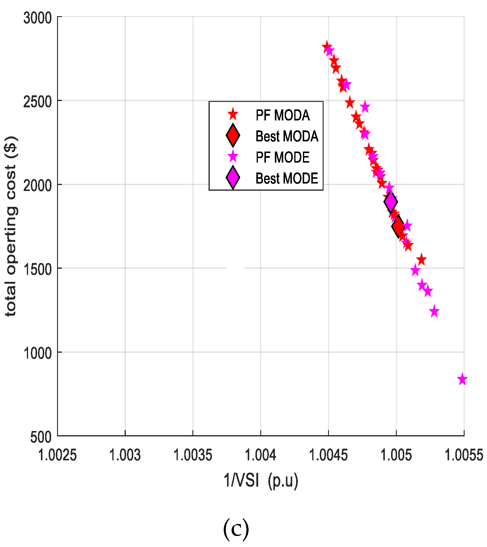The Pareto solutions for proposed algorithms at 160% loading condition are shown in Figure 3, the Pareto fronts, (PF)obtained by MODA is better than that of MODE as it produces wider Pareto fronts.

5.2. IEEE 69-Bus Power System

The IEEE 69-bus power system includes 69 buses and 68 branches. The MVA and kV base of the test system are 100 MVA and 12.66 kV, respectively. The power loss of this case is 225 kW and 102.2 kVA respectively. The data of the system are drawn from [27,28]. The optimal allocation of DGs obtained by different optimization algorithms is shown in

Table 6. Optimization results for IEEE 69-bus system.

Scenario #	Methods	MT Size (Location)	FC Size (Location)	WT Location	${\mathbf{f}}_1\left(\mathbf{KW}\right)$	${\mathbf{f}}_2\left(\mathbf{PU}\right)$	${\mathbf{f}}_3(\$)$
scenario 4	Without DG	-	-	-	51.6	1.0001	-
	MODA	0.011262 (19) 0.027492 (56)	0.08873 (61) 0.04967 (35)	35, 61	44.97998	0.99603	1065.665
	MODE	0.073422 (28) 0.019328 (23)	0.14406 (62) 0.02635 (16)	4, 68	40.67952	1.00006	1751.8986
scenario 5	Without DG	-	-	-	225	1.0001	-
	MODA	0.040926 (20) 0.020754 (58)	0.043665 (3) 0.11717 (62)	57, 3	198.4956	1.00013	2078.6976
	MODE	0.063591 (18) 0.064197 (44)	0.13501 (35) 0.10894 (63)	53, 30	202.5653	0.98754	2978.7364
scenario 6	Without DG	-	-	-	652.5	1.0002	-
	MODA	0.025213 (21) 0.017038 (27)	0 (21) 0.16383 (57)	52, 52	614.2795	1.00022	3655.0761
	MODE	0.070847 (65) 0.025387 (63)	0.11506 (35) 0 (63)	17, 29	616.5539	0.99265	3852.5329

. The optimal allocation of the DGs is based on developing the study objectives; which are improving the voltage stability index, minimizing the transmission power losses, and reducing the operating costs.

5.2.1. Scenario 4: Light Loading

The behavior of MODA is better than the behavior of MODE technique for minimizing the total operating cost and improving voltage stability index, the second objective in this scenario is reduced from 1.0001 PU obtained from an initial condition (without using DG) to 0.99603 PU. The Pareto fronts of combination of multi-objectives obtained by different optimization algorithms with light loading are shown in Figure 4. The Pareto fronts obtained by MODA are better than those by MODE as it produces wider Pareto fronts near the central point.

5.2.2. Scenario 5: Normal Loading

The minimum power loss and the total operating cost are obtained by MODA, the best locations to place the DG are buses 20, 58, 3, 62, and 57 to reduce power loss by 11.78%. Figure 5 shows three objective functions together in three dimensional diagrams.

5.2.3. Scenario 6: Heavy Loading

The performance of MODA is the best to minimize the power losses and the total operating cost, the power loss reduced by 5.86%, and the saving in the cost objective obtained from MODA method and MODE method is $197.4568. The Pareto solutions for proposed algorithms with 160% of base loading condition are shown in Figure 6.

6. Conclusions

This article presents a comparative study of two optimization techniques that have been suggested to determine the optimum location for distributed generation (DG) in electric grid systems including the minimum of a multi-objective function considering the total power loss, total operating cost, and improving voltage stability index. The suggested techniques are examined on IEEE 33-bus, and 69-bus radial distribution system. This algorithm is applied to various scenarios, including load levels (light, normal, and heavy load) and uncertainty caused by the wind energy source. The PEM is implemented for representing the wind power uncertainties. It is observed from the obtained results that the performance of MODA is better than the performance of MODE for minimizing power loss and voltage stability index in IEEE 33-bus. In 69-bus, the minimum power loss and total operating cost are obtained by MODA algorithm.

References

- Sarda, J.; Pandya, K. Optimal Active–Reactive Power Dispatch Considering Stochastic Behavior of Wind, Solar and Small-Hydro Generation. In Applications of Artificial Intelligence Techniques in Engineering; Springer: Singapore, 2019; pp. 255–263. [Google Scholar] [CrossRef]
- Bizon, N.; Lopez-Guede, J.M.; Kurt, E.; Thounthong, P.; Mazare, A.G.; Ionescu, L.M.; Iana, G. Hydrogen Economy of the Fuel Cell Hybrid Power System optimized by air flow control to mitigate the effect of the uncertainty about available renewable power and load dynamics. Energy Convers. Manag. 2019, 179, 152–165. [Google Scholar] [CrossRef]
- ChithraDevi, S.A.; Lakshminarasimman, L.; Balamurugan, R. Stud Krill herd Algorithm for multiple DG placement and sizing in a radial distribution system. Eng. Sci. Technol. Int. J. 2017, 20, 748–759. [Google Scholar] [CrossRef] [Green Version]
- Jagtap, K.M.; Khatod, D.K. Novel approach for loss allocation of distribution networks with DGs. Electr. Power Syst. Res. 2017, 143, 303–311. [Google Scholar] [CrossRef]
- Castro, J.R.; Saad, M.; Lefebvre, S.; Asber, D.; Lenoir, L. Coordinated voltage control in distribution network with the presence of DGs and variable loads using pareto and fuzzy logic. Energies 2016, 9, 107. [Google Scholar] [CrossRef]
- Dinakara Prasad Reddy, P.; Veera Reddy, V.C.; Gowri Manohar, T. Optimal renewable resources placement in distribution networks by combined power loss index and whale optimization algorithms. J. Electr. Syst. Inf. Technol. 2018, 5, 175–191. [Google Scholar] [CrossRef]
- Ali, E.S.; Elazim, S.A.; Abdelaziz, A.Y. Optimal allocation and sizing of renewable distributed generation using ant lion optimization algorithm. Electr. Eng. 2018, 100, 99–109. [Google Scholar] [CrossRef]
- Taher, S.A.; Karimi, M.H. Optimal reconfiguration and DG allocation in balanced and unbalanced distribution systems. Ain Shams Eng. J. 2014, 5, 735–749. [Google Scholar] [CrossRef] [Green Version]
- Haddadian, H.; Noroozian, R. Multi-microgrids approach for design and operation of future distribution networks based on novel technical indices. Appl. Energy 2017, 185, 650–663. [Google Scholar] [CrossRef]
- Ravadanegh, S.N.; Oskuee, M.R.J.; Karimi, M. Multi-objective planning model for simultaneous reconfiguration of power distribution network and allocation of renewable energy resources and capacitors with considering uncertainties. J. Cent. South Univ. 2017, 24, 1837–1849. [Google Scholar] [CrossRef]
- Abdolahi, A.; Salehi, J.; Samadi, G.F.; Safari, A. Probabilistic multi-objective arbitrage of dispersed energy storage systems for optimal congestion management of active distribution networks including solar/wind/CHP hybrid energy system. J. Renew. Sustain. Energy 2018, 10, 045502. [Google Scholar] [CrossRef]
- Zhang, L.; Yang, H.; Lv, J.; Liu, Y.; Tang, W. Multiobjective Optimization Approach for Coordinating Different DG from Distribution Network Operator. J. Electr. Comput. Eng. 2018, 2018, 4790942. [Google Scholar] [CrossRef]
- Wang, S.; Wang, K.; Teng, F.; Strbac, G.; Wu, L. An affine arithmetic-based multi-objective optimization method for energy storage systems operating in active distribution networks with uncertainties. Appl. Energy 2018, 223, 215–228. [Google Scholar] [CrossRef]
- Karimyan, P.; Gharehpetian, G.B.; Abedi, M.; Gavili, A. Long term scheduling for optimal allocation and sizing of DG unit considering load variations and DG type. Int. J. Electr. Power Energy Syst. 2014, 54, 277–287. [Google Scholar] [CrossRef]
- Saksornchai, T.; Eua-arporn, B. Load variation impact on allowable output power of distributed generator with loss consideration. IEEJ Trans. Electr. Electron. Eng. 2012, 7, 46–52. [Google Scholar] [CrossRef]
- Kaur, N.; Jain, S. Multi-objective optimization approach for placement of multiple dgs for voltage sensitive loads. Energies 2017, 10, 1733. [Google Scholar] [CrossRef]
- Tolba, M.; Rezk, H.; Tulsky, V.; Diab, A.; Abdelaziz, A.; Vanin, A. Impact of Optimum Allocation of Renewable Distributed Generations on Distribution Networks Based on Different Optimization Algorithms. Energies 2018, 11, 245. [Google Scholar] [CrossRef]
- Aghajani, G.R.; Shayanfar, H.A.; Shayeghi, H. Demand side management in a smart micro-grid in the presence of renewable generation and demand response. Energy 2017, 126, 622–637. [Google Scholar] [CrossRef]
- Moradi, M.H.; Mohsen, E.; Mahdi, H.S. Operational strategy optimization in an optimal sized smart microgrid. IEEE Trans. Smart Grid 2015, 6, 1087–1095. [Google Scholar] [CrossRef]
- Alavi, S.A.; Ahmadian, A.; Aliakbar-Golkar, M. Optimal probabilistic energy management in a typical micro-grid based-on robust optimization and point estimate method. Energy Convers. Manag. 2015, 95, 314–325. [Google Scholar] [CrossRef]
- Mirjalili, S. Dragonfly algorithm: A new meta-heuristic optimization technique for solving single-objective, discrete, and multi-objective problems. Neural Comput. Appl. 2016, 27, 1053–1073. [Google Scholar] [CrossRef]
- Storn, R.; Price, K. Differential evolution—A simple and efficient heuristic for global optimization over continuous spaces. J. Glob. Optim. 1997, 11, 341–359. [Google Scholar] [CrossRef]
- Robič, T.; Filipič, B. Differential evolution for multiobjective optimization. In International Conference on Evolutionary Multi-Criterion Optimization; Springer: Berlin/Heidelberg, Germany, 2005; pp. 520–533. [Google Scholar] [CrossRef]
- Hadidian-Moghaddam, M.J.; Arabi-Nowdeh, S.; Bigdeli, M.; Azizian, D. A multi-objective optimal sizing and siting of distributed generation using ant lion optimization technique. Ain Shams Eng. J. 2018, 9, 2101–2109. [Google Scholar] [CrossRef]
- Mustaffa, S.S.; Musirin, I.; Zamani, M.M.; Othman, M.M. Pareto optimal approach in Multi-Objective Chaotic Mutation Immune Evolutionary Programming (MOCMIEP) for optimal Distributed Generation Photovoltaic (DGPV) integration in power system. Ain Shams Eng. J. 2019. [Google Scholar] [CrossRef]
- Hassan, A.A.; Fahmy, F.H.; Nafeh, A.E.S.A.; Abu-elmagd, M.A. Hybrid genetic multi objective/fuzzy algorithm for optimal sizing and allocation of renewable DG systems. Int. Trans. Electr. Energy Syst. 2016, 26, 2588–2617. [Google Scholar] [CrossRef]
- Baran, M.E.; Wu, F.F. Network reconfiguration in distribution systems for loss reduction and load balancing. IEEE Trans. Power Deliv. 1989, 4, 1401–1407. [Google Scholar] [CrossRef]
- Mekhanet, M.; Mokrani, L.; Lahdeb, M. Comparison between three metaheuristics applied to robust power system stabilizer design. POWER 2012, 9, 10. [Google Scholar]
Figure 1.
Pareto solutions at light loading. (a) Pareto solutions in three dimensions (. (b) Pareto solutions in two dimensions (. (c) Pareto solutions in two dimensions (.
Figure 2.
Pareto solutions at normal loading. (a) Pareto solutions in three dimensions (. (b) Pareto solutions in two dimensions ( (c) Pareto solutions in two dimensions (.
Figure 3.
Pareto solutions at heavy loading. (a) Pareto solutions in three dimensions (f1, f2, f3). (b) Pareto solutions in two dimensions ( (c) Pareto solutions in two dimensions (.
Figure 4.
Pareto solutions at light loading. (a) Pareto solutions in three dimensions ( (b) Pareto solutions in two dimensions ( (c) Pareto solutions in two dimensions (.
Figure 5.
Figure 6.
Pareto solutions at light loading. (a) Pareto solutions in three dimensions (. (b) Pareto solutions in two dimensions (.