4.2.1. Basic Network Properties
Before we could identify the features of a network, it was essential to determine fundamental properties relating to its size. In this study, information about the size of all the networks is described in terms of the number of stations and links in them. As shown in
Table 2, the integrated network is significantly the largest among the three networks as it has the highest number of stations and links. The bus network follows in the second place, and then the subway network. The observation suggests that the integrated network provides higher accessibility to destinations, owing to the high number of routes and connections created as a result of combining both bus and subway networks.
We compared the network diameter (
) of the three networks. Network diameter is a measure of the longest graph distance that exists between any two nodes in a network. It is obtained by finding the maximum distance of the shortest paths between the stations in the network. This is expressed mathematically as
where
is the number of links in the shortest path from station
to station
We noticed that the subway network’s diameter was the lowest. The observation is understandable as the size of the subway network is the smallest among the three networks, considering that it has the lowest number of stations (). A more striking point to note is that, even though the integrated network is larger than the bus network, its diameter is significantly smaller than that of the bus network’s diameter. It indicates that integrating the subway and bus network significantly reduces the travel distance within the network, even though it is much more extensive.
Another vital network property that is based on the relationship between the elements of a network (stations and links) is the degree of connectivity (
). The connectivity indicator is very useful to transport planners and practitioners as it estimates how easy it is to travel from one station to another in a network based on the level of connectivity. We measured the degree of connectivity using the gamma index calculated as the ratio of the actual number of links over the maximum number of links in the network [
31]:
where
is the number of links and
is the number of stations in the transportation network.
We observed that the degree of connectedness was highest in the subway network (
). On the other hand, the integrated network, which was larger than the bus network, had the second-highest degree of connectedness (
). Based on the results of the underlying basic network properties displayed in
Table 2, we infer that it is more beneficial to travel using the integrated public transportation network as it services a larger coverage area and provides more effortless movement between stations compared to the bus network.
4.2.2. Average Path Length and Clustering Coefficient
The average path length (
) for all the networks analyzed in this study was calculated to determine the average number of links traversed along the shortest paths of all possible pairs of stations within the network. This relationship is formally stated as
where
is the average path length,
is the number of nodes in the network, and
is the length of the shortest path between stations
and
.
We identified that the average path length of the subway network was the lowest due to its small size. The integrated network, which is somewhat broader among the three, had the second lowest average path length. An important point to note is that, even though the integrated network is larger than the bus network, the integrated network showed a significantly smaller diameter and average path length. The average path distance in the bus network is 1.5 times longer than that of the integrated network. It signifies that using the integrated network is much advantageous as the travel distance between the farthest stations is lesser even though its network is much larger.
The measure of cohesiveness or intraconnectivity among neighbors of a node
(nodes connected by a single link), described as its clustering coefficient, was also determined [
61]. If a node
has
neighbors, then its clustering coefficient,
, is expressed as
where
is the number of links between node
i’s neighbors and the normalization factor
is the maximum number of links that could exist among its neighbors. For network comparisons, the overall level of clustering within the network was further determined by averaging
over all the nodes in the network,
.
The range of clustering coefficients for individual stations in both subway and integrated networks were within the interval , whereas that of the bus network was because of the normalization factor in the formula. Overall, it is essential to note that the average clustering coefficient of the integrated network was higher compared to the other networks, indicating the presence of a higher number of tightly knitted groups within the integrated network.
Both the average path length (
) and average clustering coefficient
) of a network play critical roles in identifying “small-worldness” properties of a network. Researchers in the transportation field have noted small-world networks as those that show high connectivity and high capability of linking communities more efficiently (short characteristic path length), while being less redundant. In terms of infrastructural resilience, one significant advantage of investigating this property is to analyze how fault-tolerant and structurally robust a transport network can be in times of disruptions [
7]. To check the presence of the small-world phenomenon in our networks, we compared their average clustering coefficient and average path length to similar Erdos–Renyi (E–R) random networks constructed using the same number of stations in each target network, as proposed in the literature [
7,
32,
56,
62].
As described in
Table 3 below, we found that, apart from the average clustering coefficient of the integrated network, those of the subway and bus networks were lesser than their corresponding values from their equivalent E–R random networks. However, the average path lengths of all the E–R random networks were orders of magnitudes lower than in their corresponding real networks. From the comparisons, we conclude that none of the three networks show characteristics of small-world networks. The results show that the networks are not fault-tolerant in terms of connectivity and cannot maintain connectivity between stations in case of disruptions. Chopra et al. [
7] reached similar conclusions as they discovered that the London metro network was not a real-world network.
Furthermore, we analyzed the node degree distributions of the individual networks to identify whether or not they are scale-free. Node degree distributions help in understanding the structure of complex networks. In scale-free networks, the degree distributions (the probability that a station has
degrees) follow a power law,
which suggests that stations with a higher number of connections have a strong influence on their networks’ structure and dynamics. Such distributions are characterized by a more gradual fall, which is different compared to the exponential distribution. The scale parameter
shows how the tail of the distribution of
falls. It mostly lies within the range
(scale-free regime); however, it could be
[
7]. Networks with these properties are free of any characteristic scale, implying that they maintain the same underlying structure, even as the network grows [
63].
The study of scale-free networks can help us determine how resilient or robust a network is, and to identify and control important hubs [
33]. We analyzed the probability distribution of station degrees by plotting them on a double logarithmic scale. We employed maximum likelihood estimation and goodness of fit tests (Kolmogorov–Smirnoff tests) to determine the parameter
and to test how well the data fit the power law distribution, respectively. The hypothesis that data follow the power law distribution is plausible if
p-value
.
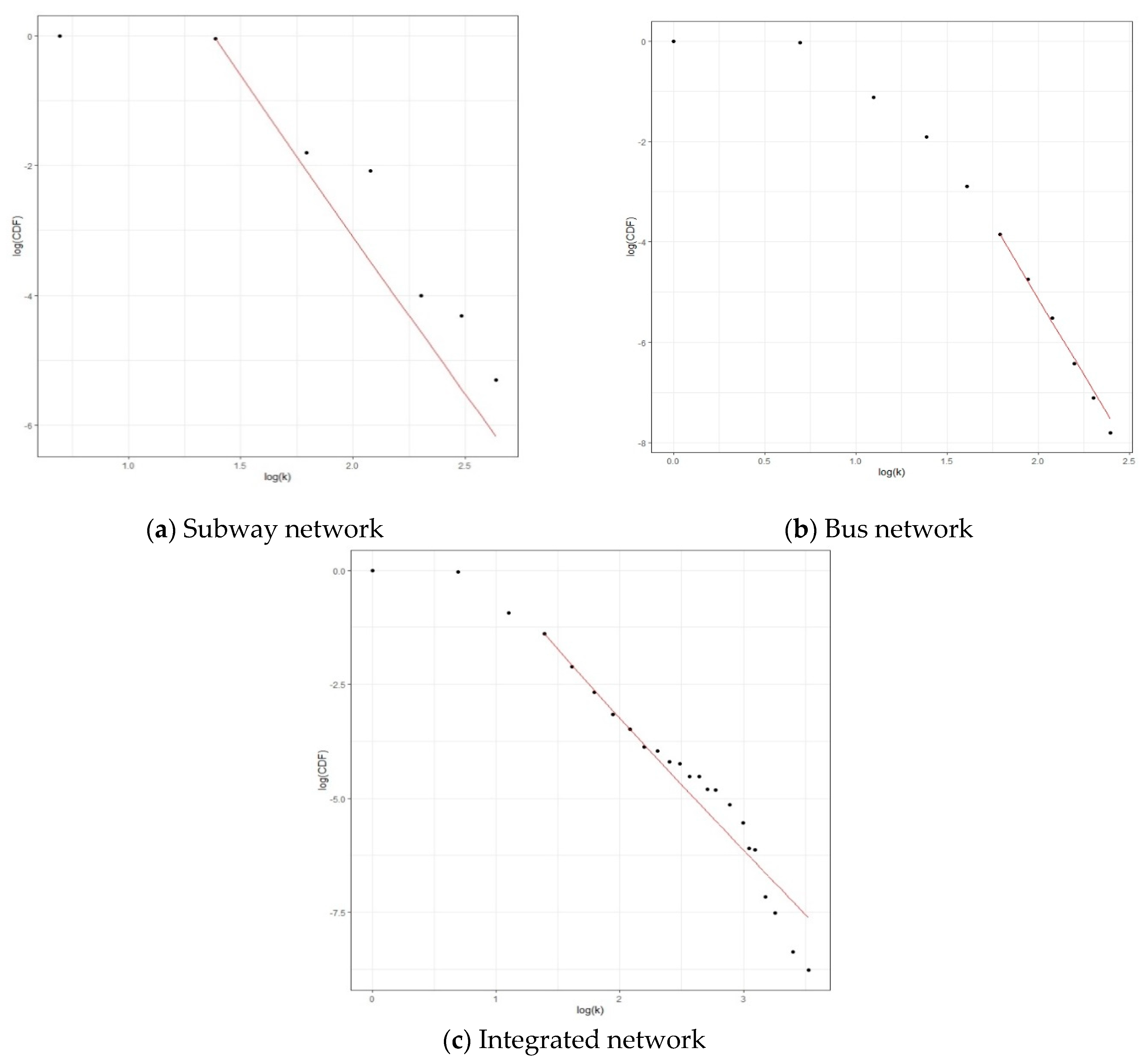
By fitting our data to the power law distribution shown in
Figure 3, we determined that only the bus networks’ dataset followed the power law distribution since its
p-value was 0.1298 (
p-value
). Hence, the probability of finding a station with
connections is proportional to
, illustrating that the bus network has excessively high-degree stations (hubs). The observation suggests that it is more robust to network breakdowns; however, a significant drawback is that it is more vulnerable to attacks compared to the subway and integrated networks. The results for the scale-free detection and the graphs for the power law distribution of the subway, bus, and integrated networks are shown in
Table 4 and
Figure 3 below.
4.2.3. Community Detection within the Networks in the SMA
In order to analyze the community structure of the networks and identify cascading impacts resulting from disruptions, we analyzed the various communities that exist within each network using the idea of modularity in graph theory. Modularity is used to determine the strength of the segregation of a network into communities [
64]. It could be explained as the proportion of links that fall within the given community minus the expected proportion if links were randomly spread. The equation for modularity,
is given as;
where
is the proportion of ends of links that are attached to the stations in a community
,
is the proportion of ends of links that are attached to stations in community
, and
. High modularity reflects that there are more links in the community than was expected by chance.
(positive) if the number of links within the community exceeds the expected number of edges of that community.
In transport networks, the communities identified show the different transit operation zones [
5]. A transport network with high modularity is preferred as its communities have dense connections between stations within the same community, but have sparse connections between stations in different communities. This results in more efficient passenger flow within each community with high modularity compared to passenger flows between communities. As such, transport planners use this information to identify patterns of vulnerability and to improve the resilience of networks.
We employed a community detection algorithm known as the Louvain algorithm, first published by Blondel et al. [
65], due to its ease of implementation. The algorithm is a greedy optimization technique that consists of two phases. The first phase involves searching and grouping of nodes based on the gains of modularity that result when a node
is moved from one community and placed in another community. The first phase stops when no node can be moved to any other community to improve the modularity. The gain in modularity is achieved by relocating a node
into a new community
and it is computed by the formula below:
where
represents the total sum of link weights in the network,
is the sum of weights of links incident to node
,
represents the sum of weights belonging to links connecting node
and other nodes in the new community
,
denotes the sum of weights belonging to links that are incident to nodes in the new community
, and
is the sum of weights of links in the new community
. The second phase involves the building of a new network such that the nodes are the communities. The steps described above are iterated until a maximum modularity for each community is achieved such that no further improvement can be obtained.
The community detection results displayed in
Table 2 show the presence of communities spread across the various networks. As many as 63 communities were identified in the bus network, whereas 59 and 23 communities were detected in the integrated and subway networks, respectively. In general, the modularities for communities across all networks examined in this study are highly dense as their modularity values are almost 1 (
. The communities in the bus and integrated networks were identified to be almost equal and highly dense compared to the subway network.
From the results, we observe that the communities in the bus and integrated networks are closely connected, suggesting a faster rate of movement and increased accessibility, which is preferred in transport networks. In terms of the impacts of disruptions, they are robust against breakdowns due to the high connectivity. As such, if a link is disrupted, passengers could be rerouted through adjacent links in the community to their final destinations. In that way, traffic flows within communities would not be significantly affected.
4.2.5. Centrality and Connectivity in the Public Transportation Networks in the SMA
Many researchers have studied the centrality of stations in transport networks as it shows the value of stations in networks. Some studies have described node centrality as either “important” or “influential” nodes in a network [
2,
27,
31]. In this study, we identified central stations in all of the three networks based on commonly used centrality measures such as degree centrality, betweenness centrality, closeness centrality, eigenvector centrality, and eccentricity centrality.
The degree of a node is the most basic and straightforward centrality measure. It reflects the number of links that are directly connected to a station
in the network [
31]. Hence, the higher the degree of a station, the higher its connectivity and the more accessible it is. This translates into the stations capacity to increase the chance of receiving many passenger flows. Also, the average degree of a network shows, on average, how connected each node in the network is. Transport authorities are interested in this metric as it shows how accessible the nodes in a transport network are. For a given station
, with
as its indicator variable in the
adjacency matrix (which shows
if a connection exists between nodes
and
, the station degree
and its network-wide average degree
are given as
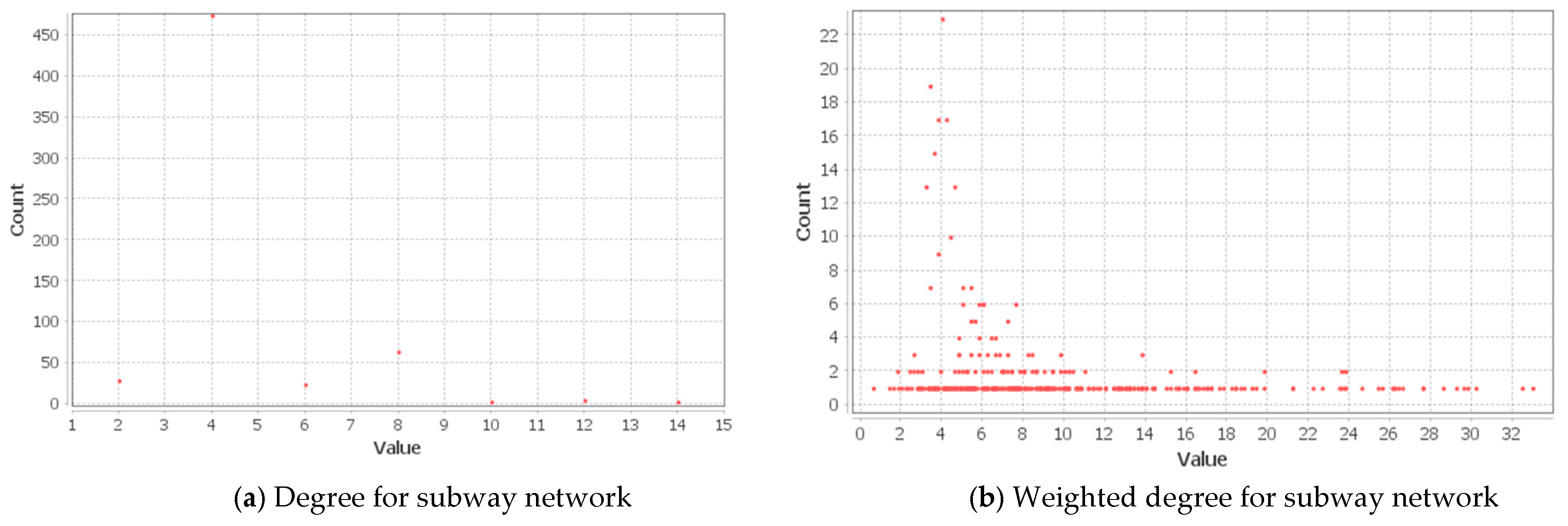
The nodes in the subway network had a minimum degree of 2 and a maximum degree of 14. Both the bus and integrated networks had a minimum degree of 1 each, and maximum degrees of 11 and 34, respectively. On comparing the three networks, the integrated network had the highest maximum degree of 34, which is a result of the integration of both bus and subway networks. Overall, the subway network had the highest average degree of 4.6. Both the bus and integrated networks also had high average degrees of 2.5 and 3.0, respectively. Since the stations in the integrated network show high degrees, we can infer that it is more connected and has higher access to various destinations in the network.
In this paper, we used a weighted network, where each link has a weight expressed in terms of the inversed distance between two stations connected by a common link. Hence, in order to identify the effect of distances and connections on station importance (in terms of degree), the weighted degree or station strength was analyzed by summing the weights of the links incident to the station in question [
27,
30,
68,
69,
70,
71]. For station
, its weighted degree
is a measure of how strong and directly connected it is in a network. The networks’ average weighted degree was also determined for comparison of the three networks using the formula;
A station with a higher weighted degree denotes one with high proximity. Due to its importance, it is expected to have high passenger flow volume. We observed a positive relationship between the average weighted degree measure and network size. We identified that the average weighted degree value of the integrated network was the highest and the subway network had the lowest. Hence, on average, the links in the integrated network are much shorter compared to those in the bus network. This observation shows that stations in the integrated network can offer the easy movement of people in terms of accessibility since they are more connected and closer to each other [
27].
We further analyzed the degree measure by plotting and comparing the graphs of the frequency of all stations’ degrees in the three networks. The plots in
Figure 4 show that both bus and integrated networks’ graphs are right skewed with modes of three. The subway network’s degree distribution, on the other hand, shows a mode of four, with few stations having high degrees due to its small size. It also shows that most of the subway stations have low degree values. The highest occurring degree value in both networks is two. However, due to the large network size, the degree distribution of the integrated network had the most extended tail, signifying a high chance of finding hubs (excessively high-degree stations) within the network. The graphs of the frequency of stations’ weighted degrees in all three networks are right-skewed, with most stations appearing to have weighted degree values from 0 to 20. The highest occurring weighted degree in the subway network is 3.8, and both bus and integrated networks have a weighted degree mode of 7.48. Similar trends were observed in the graphs for the degree values. Fewer stations having higher weighted degrees in integrated networks show that few stations have very high proximity. This observation affirms that integrating the networks will improve accessibility. The degree and weighted degree distributions of the subway, bus, and integrated networks are visualized in
Figure 4.
The betweenness centrality measure shows how many times a station comes in between the shortest paths of stations within a network. Betweenness centrality
for a station
on shortest paths connecting nodes
and
is defined as follows;
where
is the total number of shortest paths connecting nodes
and
and
is the number of these paths that go through station
. The numerator should be as high as possible to achieve a high betweenness centrality.
A public transportation facility with the highest centrality is an active player that serves as an important transfer point or connector to many regions within the transport network. Many flows will have to go through this station in order to reach other locations in the network. To make comparisons between networks with different sizes, we used the normalized form of the betweenness centrality [
40]. From
Table 5 below, the network with the lowest average betweenness centrality is the integrated network
and the system with the highest average betweenness centrality is the subway network
. The bus network comes in between with an average betweenness of 0.003. The results show that the average betweenness centrality of stations in the SMA’s public transportation network decreases with increasing network size.
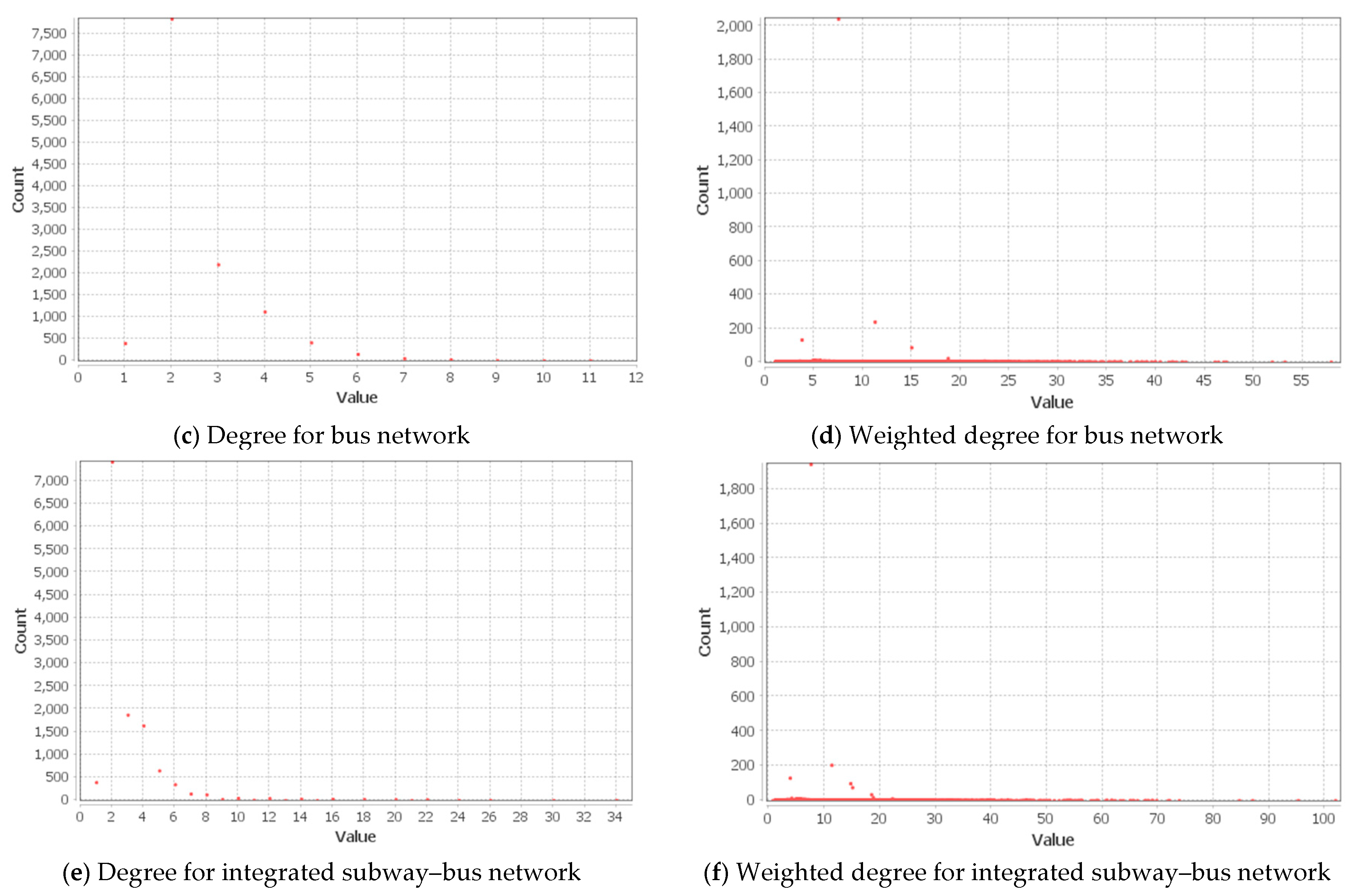
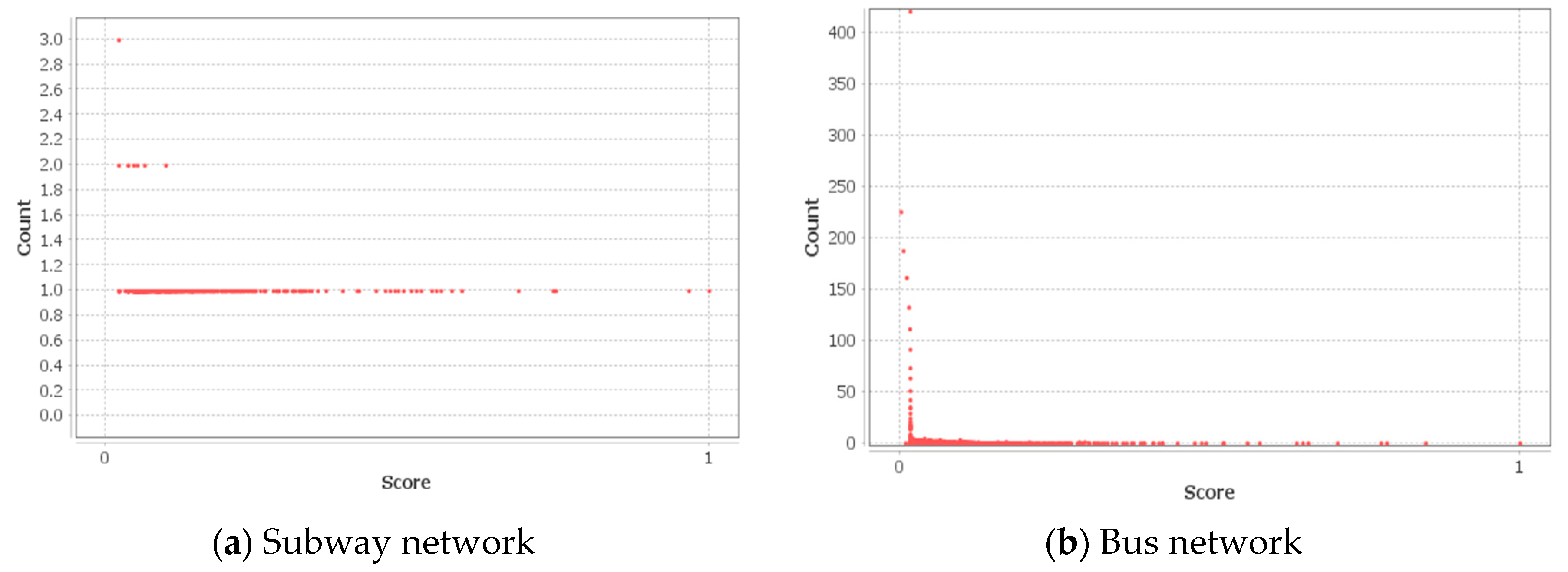
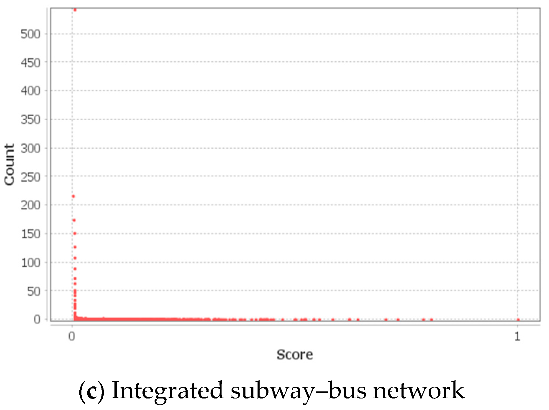
The distribution of the station betweenness centralities in the subway network, as seen in
Figure 5, shows that many stations in the subway network have betweenness centrality of zero and there is a steep drop towards the right (right-skewed). In the bus and integrated networks, the points are clustered in the vicinity of the origin. Also, the subway network has 34% of its stations having a betweenness greater than the total average betweenness centrality, 23% of stations in the bus network had betweenness centralities higher than the average, and 17% of the stations in the integrated network have betweenness higher than the average. Since, on average, the betweenness centrality of the subway is higher than both bus and integrated networks, we can conclude that its stations are strategically placed and connect several regions in the network more effectively.
Figure 5 below shows the betweenness centrality distributions for the subway, bus, and integrated networks.
The average distance from a given starting node
to all other nodes, known as closeness centrality
is defined by the equation:
where
is the shortest distance between nodes
and
, and
is the number of stations in the network. Closeness centrality describes how easy and fast a station can be reached in terms of speed and frequency compared to other stations in a transport network. The idea is that the higher the closeness centrality of a station, the closer it is to other nodes and it takes the least number of steps to reach them.
Normalized closeness centrality values in
Table 5 above show that the integrated network has the highest average closeness centrality
followed by the bus network
in the second place, and finally the subway network
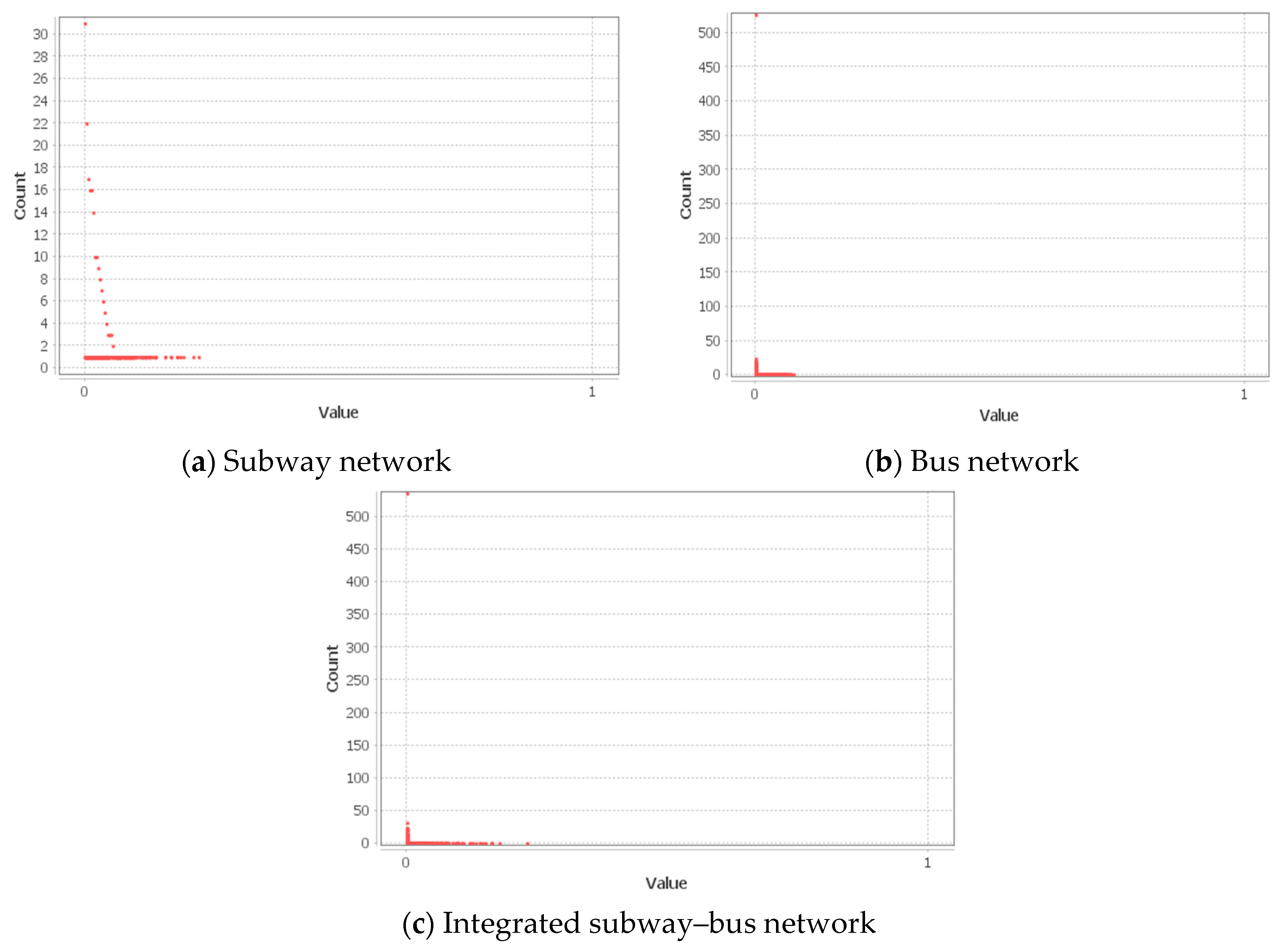
. A glance at the distribution of closeness centrality of stations visualized in
Figure 6 also presents interesting observations.
The points in the subway networks distribution are dispersed away from the origin with a mode of 0.048, and many stations have very low closeness centralities. The most common closeness centrality value in both the bus and integrated networks is zero (0), showing a right-skewed distribution with their centrality values tapering slowly downwards, depicting that many stations have higher closeness centralities. The proportion of stations in the subway network with a closeness centrality score higher than the average is 49%. That of the bus and integrated networks are 12% and 10%, respectively.
Overall, the average closeness centrality metric trends of the three networks clearly illustrate that the average closeness centrality of stations in the SMA increases with network size. The observations show that movement from one station to another is easier and faster in the bus and integrated networks. Again, this shows that the structure of the subway network is improved to offer faster movements when it is combined with the bus network. Hence, employing integrated networks is imperative for making public transportation usage more time saving, efficient, and accessible. Graphs for closeness centrality distributions for the three networks are shown in
Figure 6.
The eccentricity of a station
captures the maximum distance between it and the farthest station from it, and the inverse of the eccentricity of a station is its eccentricity centrality metric [
44]. Formally, if
is a station in a connected network
, and
is the shortest path between stations
and
, then the eccentricity of station
,
is given as
The reciprocal of eccentricity
of station
is its eccentricity centrality
:
As closeness centrality indicates how close a station is to all other stations in the transport network, eccentricity centrality shows how close the farthest station is away from a given station in a network. Thus, a station with a high eccentricity measure is a long way away from the farthest station from it, and a station with a high eccentricity centrality assumes high station proximity (very accessible). The eccentricity centrality values in
Table 5 show that, on average, the maximum distances between the subway stations are short, making them very reachable. The integrated network follows in the second place, showing that integrating both bus and subway networks improves the accessibility of stations in the subway network.
We observed that there are several centrality measures that show the importance of stations by either the quantity of links incident on it (degree centrality), the sum of weights of the links incident on it (weighted degree or strength centrality), or based on the paths in the network (betweenness, closeness, and eccentricity centralities). Besides these measures, we consider the eigenvector centrality, whose underlying principle is based on the “quality” of its connections and not only the number of its adjacent stations [
27,
72]. As such, a station that is connected to a highly central station is more important than another station that is connected to a less important station.
For a graph
with
and adjacency matrix
the relative centrality score of station
can be formally expressed as the positive multiple of the sum of adjacent centralities:
where
is the constant. By using matrix algebra, the above equation satisfies the eigenvector equation
.
is an eigenvector of
if
is a scalar multiple of
As there are multiple eigenvectors, the value of
that corresponds to the largest value of
is the eigenvector centrality measure.
Again, as we want to compare centralities across different networks, we normalized the eigenvalue centrality values. From
Table 5 above, a trend similar to that of the average betweenness centrality is observed in the case of the average eigenvector centrality. The average eigenvector centrality gradually decreased with the size of the network. Considering the subway network, which has 602 stations, the average eigenvector centrality measure was 0.11, followed by the bus network
which had an average eigenvector centrality measure of 0.03. The integrated network, with the largest number of stations
had the lowest eigenvalue centrality value of 0.02.
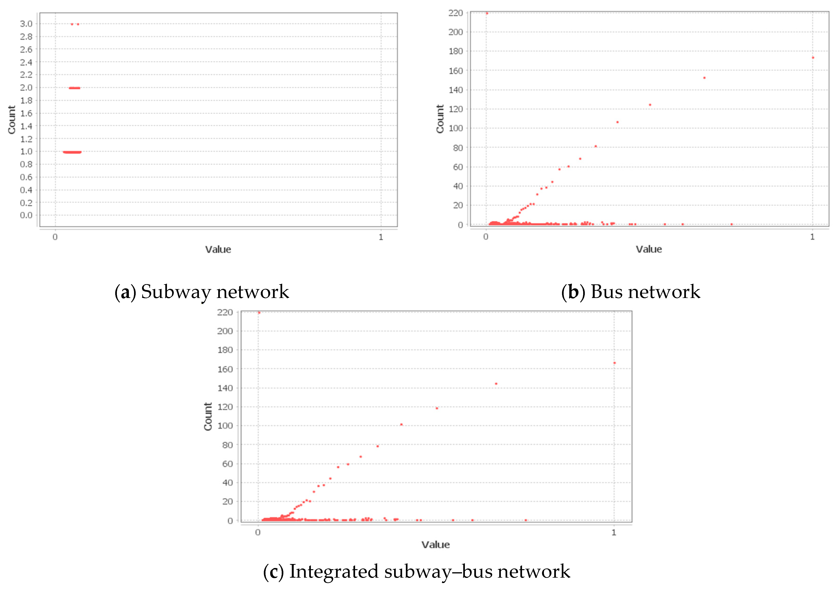
We proceeded with further analysis and noted that more than 70% of the stations in all the networks had eigenvector centralities less than their average values (
). That means less than 30% of stations in the networks were connected to highly central nodes. The eigenvector centrality distributions in the integrated network show that many stations clustered around the origin (mode = 0.003), meaning there are many stations connected with less important stations. A similar trend is observed in the bus network; however, the points seem a little bit more dispersed away from the origin (mode = 0.014). The eigenvector centrality distribution in the subway network shows that a high proportion of the stations in the subway network had higher centrality values (mode = 0.019).
Figure 7 shows graphs of eigenvector centrality distributions of the subway, bus, and integrated networks.
From
Table 6, we observed that on average, even though the bus network is bigger compared the subway network, the degree, weighted degree, and eigenvector centrality values for nodes that provide intermodal connections (bus to subway or subway to bus integrated networks) were higher compared to nodes with only bus to bus connections. Unlike the bus network, the much smaller subway network consists of many transfer stations, such that commuters can use other subway lines to reach their destination. The other metrics (closeness centrality and betweenness centrality were comparable. Hence, we can infer that the bus station importance (based on degree, weighted degree, and eigenvector centrality) increases to a larger extent when it is integrated with the subway network, since it benefits from the subway network’s abundant transfer opportunities. This result shows that connecting bus stops with subway stations further increases accessibility.
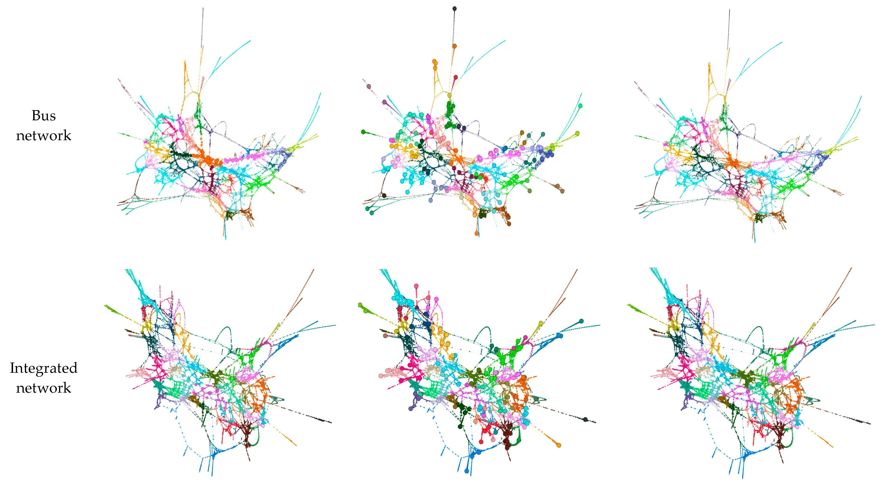
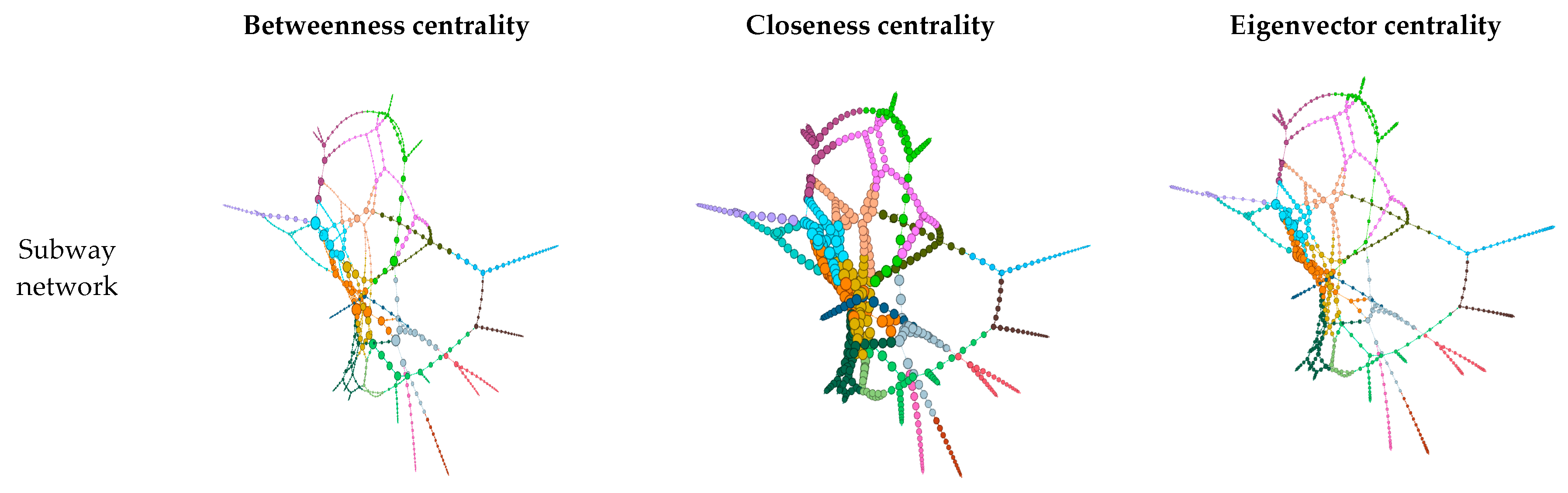
To show the spatial distribution of stations, the station centrality measures for the three network types studied in this research are plotted together with the community detection results in
Figure 8. The colors represent the various communities in the network where the service providers mostly operate and the magnitude of the centrality measure can be seen in terms of the size of the stations. The larger the size of the station, the higher its centrality.


