The Derivation of Cooling Set-Point Temperature in an HVAC System, Considering Mean Radiant Temperature

Abstract

Heating, ventilation, and air-conditioning (HVAC) systems usually have a set-point temperature control feature that uses the indoor dry-bulb temperature to control the indoor environment. However, an incorrect set-point temperature can reduce thermal comfort and result in unnecessary energy consumption. This study focuses on a derivation method for the optimal cooling set-point temperature of an HVAC system used in office buildings, considering the thermal characteristics and daily changes in the weather conditions, to establish a comfortable indoor environment and minimize unnecessary energy consumption. The operative temperature is used in the HVAC system control, and the mean radiant temperature is predicted with 94% accuracy through a multiple regression analysis by applying the indoor thermal environment data and weather information. The regression equation was utilized to create an additional equation to calculate the optimal set-point temperature. The simulation results indicate that the HVAC system control with the new set-point temperatures calculated from the derived equation improves thermal comfort by 38.5% (26%p). This study confirmed that a cooling set-point temperature that considers both the thermal characteristics of a building and weather conditions is effective in enhancing the indoor thermal comfort during summer.

1. Introduction

People currently spend 87% of their time indoors [1]. As indoor activities are conducted more frequently, occupants are attempting to create indoor thermal environments that allow them to feel comfortable [2]. Fanger defined thermal comfort as “the condition of mind that expresses satisfaction with the thermal environment” [3]. Thus, the extent to which the thermal comfort of building occupants is maintained has become an important part of a building performance evaluation [4]. In addition, it is crucial to consider not only the thermal comfort of the occupants but also a management plan to satisfy the comfort level of an indoor environment during the design and operation of a building [5].

To create a comfortable indoor environment, most buildings use a set-point temperature control in the heating, ventilation, and air-conditioning (HVAC) systems, which measures the indoor temperature of a specific space and controls it through a comparison with the set-point temperature [6]. This control usually considers the indoor dry-bulb temperature for convenience, which is the set-point temperature set by the occupant or manager [7]. However, it is insufficient to consider the thermal equilibrium or radiant heat transfer of the human body inside a building [8]. To achieve thermal comfort of the occupants, it is important to consider not only the indoor dry-bulb temperature but also different variables, such as the thermal environment’s factors, building usage, occupant characteristics, and weather conditions; however, it is not easy to satisfy every occupant in a space and control the indoor conditions simultaneously [9,10]. In addition, occupants apply trial and error to set the indoor temperature to a comfortable level, thus causing occupant discomfort and leading to unnecessary energy consumption [11,12].

More notably, because different buildings have different shapes, types of insulation, fenestrations, and window-to-wall ratios, their thermal characteristics manifest in different ways. Because the thermal characteristics of a building are a primary element, along with weather conditions, in establishing an indoor environment [5], both should be applied as key values in HVAC system controls. However, in the Republic of Korea, buildings are controlled using a one-size-fits-all model, pursuant to the laws and administrative regulations (26 °C for cooling; 20 °C for heating) to prevent excessive building energy consumption regardless of the thermal comfort of the occupants [13]. The different thermal characteristics of a building and daily changes in the weather conditions are not considered, and can potentially increase occupant discomfort and deteriorate the work productivity [6].

To overcome the limitations of conventional control, comfort controls have been studied by considering the indoor temperature and various factors of the thermal environment. A previous study defined comfort control as “maintaining a constant level of comfort throughout the entire period” [14], and many studies have applied using various thermal environment indices, including the comfort zone developed by the American Society of Heating, Refrigerating, and Air-Conditioning Engineers (ASHRAE) [8,15]; adaptive thermal comfort [16,17]; and Fanger’s predicted mean vote (PMV) model [11,12,18,19,20,21,22,23] as control criteria. The results indicate that applying comfort control is advantageous to increasing indoor comfort and reducing energy consumption, and a new direction for the progress of HVAC systems control was suggested. However, a variety of problems have emerged in terms of comfort control; e.g., measurement sensors under difficult-to-measure variables, including the air velocity, mean radiant temperature (MRT), and clothing insulation; increased maintenance costs; and a delayed processing time owing to complex computations [24,25]. For these reasons, limitations in applying comfort control to actual buildings have been shown.

Despite diverse methods being used to control HVAC systems for indoor environments, an incorrect set-point temperature may reduce the thermal comfort of the occupants and cause unnecessary energy consumption. In addition, because the thermal characteristics of a building are diverse and dealing with outdoor environments is a daily challenge, a fixed and uniform set-point temperature is not always suitable for thermal comfort, and it is not easy for the occupants or manager to determine an optimal set-point temperature for a certain building.

This study was motivated by the idea that an HVAC system should be controlled by considering the thermal characteristics of a building and the weather conditions. Therefore, this study mainly focused on a derivation method of the optimal set-point temperature when considering daily changes in the weather conditions and the thermal characteristics of an office building using an HVAC system. To achieve an advanced thermal comfort in a controlled space, this study applied the operative temperature to the set-point temperature control instead of the dry-bulb temperature. The operative temperature was defined as a uniform temperature of a radiantly black enclosure in which an occupant would exchange the same amount of heat by radiant and convection as in the actual non-uniform environment [26]. Additionally, it was dealt with as a thermal environment index that considers both the indoor temperature and the MRT, which have a significant effect on the PMV [27], among other major variables for a thermal environment. Despite agreement among the current thermal comfort standards or thermal comfort models that the MRT must be considered in an HVAC system control, it has often been a practice to avoid measuring the MRT and instead assume that it is equal to the dry-bulb temperature [28,29], due to several reasons, such as complicated MRT measurement methods [30,31,32] and a hypothesis that surrounding indoor surfaces have a uniform temperature and radiation flux [33]. However, that can lead to the incorrect determination of PMV and comfort level [28]. Although recently, various attempts have emerged to predict variables such as metabolic rate and clothing insulation, which are difficult to measure and are used as an assumed value [34,35,36,37], they are still limited when finding a way of predicting the MRT in high accuracy. Therefore, instead of directly measuring the MRT with sensors and assuming that the MRT and dry-bulb temperature are equal, this study also proposes a prediction method for the MRT; namely, an MRT regression model that applies simple datasets, including the indoor thermal environment data of the subject building and the weather information at 3-h intervals provided from the Korea Meteorological Administration (KMA) [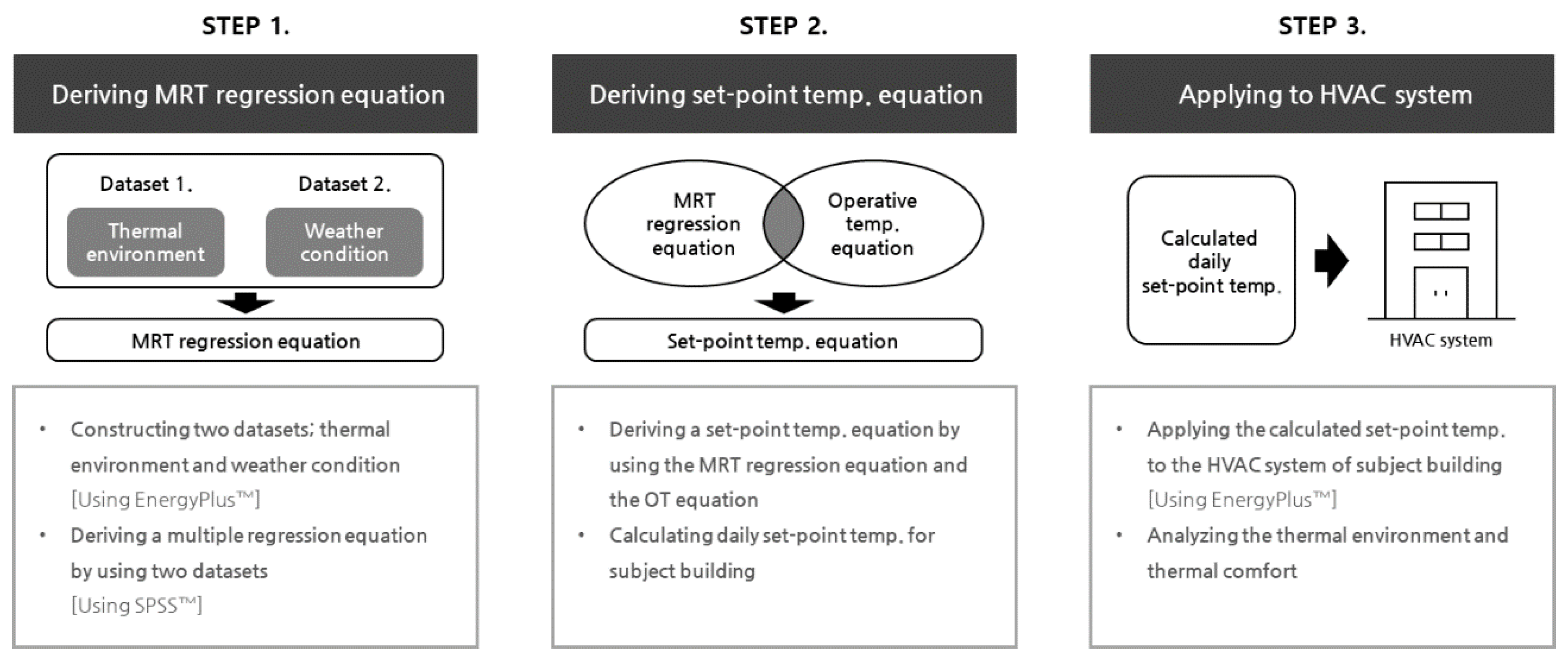38]. From combining both an MRT regression equation and the operative temperature equation, the set-point temperature equation that can maintain an operative temperature suitable for the subject building was established and applied, such that, when the weather data are input, the set-point temperature suitable for the day is able to be changed for the HVAC system. Despite the existence of other prediction methods (e.g., machine learning and artificial neural networks (ANNs)), the reason for using a regression analysis for MRT prediction is to create a set-point temperature equation that anyone can easily access while also using the operative temperature equation.

To achieve the above study objectives, this study concentrated on cooling control during summer (August) with high solar radiation. The equation used for accurately deriving the cooling set-point temperature was then developed by (i) establishing two types of datasets; namely, thermal environment and weather conditions (e.g., the indoor temperature, outdoor temperature, and sky cover) datasets; (ii) deriving significant variables for predicting the MRT; (iii) constructing an MRT regression model using the selected input variables; and (iv) deriving the set-point equation by combining the MRT regression equation and the operative temperature equation. This study aims to overcome the control limitations of a conventional HVAC system by maintaining indoor comfort and enabling energy-efficient control in buildings. The results of this study will contribute to maintaining comfortable indoor environments during the summer months.

2. Methodology

2.1. Study Process

To derive the equation of the cooling set-point temperature for the subject building, three main steps were followed, as shown in Figure 1.

In Step 1, for the subject building used in the present study, simulation modeling was implemented using a building energy dynamic analysis program, EnergyPlus version 8.6 (US Department of Energy, Washington, DC, USA, 2016). An overview and modeling of the subject building are described in Section 2.2. Subsequently, both the indoor thermal environment of the subject building and the weather data were established in each dataset. Here, the dataset indicates data on a group of several variables regarding the indoor thermal environment or the weather data, which can achieve a high accuracy when predicting the MRT; accordingly, it is important to find the appropriate variables in this study. The established dataset was implemented in the MRT regression model through the statistical program SPSS version 25.0 (SPSS Inc., Chicago, IL, USA, 2018).

In Step 2, the MRT regression equation was used to calculate the optimal set-point temperature to maintain a suitable operative temperature of the subject building. This study combined the MRT regression equation with the operative temperature equation and derived a set-point temperature equation for the subject building. Considering that the weather conditions and MRT change hourly, the suitable temperatures for each hour of the day were calculated, and the median of the calculated temperatures was used to select the set-point temperature of the day.

Finally, in Step 3, the daily set-point temperatures calculated from the above were applied to the HVAC system of the subject building through EnergyPlus. This study analyzed the characteristic changes in the indoor thermal environment and the thermal comfort after applying HVAC system control.

2.2. Subject Building

The subject of this study is an office building located in Gangnam-gu, Seoul. To achieve the purpose of this study, which considers the MRT, the subject building was deemed suitable as a location where the influence of the external environment, especially solar radiation, was applicable. This is because reflected solar radiation in HVAC indoors can significantly alter occupants’ thermal comfort and MRT gives information about the extent of this influence [29]. Thus, within the perimeter zone (which is a space to twice ceiling height from the outer wall and referred to a passive zone), the subject building can be easily affected by outdoor air and solar radiation while ensuring direct daylight and natural ventilation [39]. Hence, an office building with a higher proportion of the perimeter zone was selected as the study subject, as shown in Figure 2. In addition, Figure 3 shows the front view and simulation modeling of the subject building. The 10th floor of the building was selected as the subject floor, the indoor thermal environment and electrical energy consumption of which were analyzed in this study.

It is first necessary to set the operative temperature range suitable for the subject building. The Chartered Institution of Building Services Engineers (CIBSE) recommends maintaining an operative temperature range of 22–24 °C (PMV = ±0.25) to create a suitable thermal comfort zone for office buildings during the summer, as shown in

Table 1. Recommended design requirements for an office (Chartered Institution of Building Services Engineers, CIBSE).

Building/Room Type	Winter			Summer
	Operative Temp. [°C]	Metabolic Rate [met]	Clothing Insulation [clo]	Operative Temp. [°C]	Metabolic Rate [met]	Clothing Insulation [clo]
Office:
executive	21–23	1.2	0.85	22–24	1.2	0.7
general	21–23	1.2	0.85	22–24	1.2	0.7
open-plan	21–23	1.2	0.85	22–24	1.2	0.7

Notes: Temperature ranges based on stated values of met and clo and predicted mean vote (PMV) of ±0.25. Calculation assumes relative humidity = 50% and air velocity = 0.15 m/s.

[40]. Using this range, the target operative temperature of the subject building was set at 23 °C; i.e., the average comfort range. In addition, the air velocity was set at 0.15 m/s based on the CIBSE recommendation.

Table 2. Overview of subject building and EnergyPlus input data.

Overview of Subject Building
Location		Gangnam-gu, Seoul
Usage		Office
Light		9201 m2
Structure		Steel framed reinforced concrete
Scale		B7/14F
Simulation Conditions
Operation time		Weekday: 08:00–21:00/Weekend: off
Metabolic rate		70 W/m2
Lighting		12 W/m2
Equipment		11.8 W/m2
Occupant density		0.2 person/m2
Min. outdoor air rate		0.1 ACH
Cooling set-point temperature		26°C
Weather data		Seoul, Republic of Korea (.epw)
Building Envelope and HVAC
Wall		0.147 W/m2K
Window		1.21 W/m2K (SHGC: 0.507)
Roof		0.136 W/m2K
Floor		0.146 W/m2K
HVAC	System air conditioner	EHP indoor unit (floor)	Cooling: 60 kW
			Heating: 68 kW
		EHP outdoor unit (floor)	Cooling: 63.8 kW
			Heating: 69.3 kW
Ventilation	ERV system (floor)		2000 CMH
Input parameters of PMV
Air velocity [40]		0.15 m/s
Clothing insulation (office) [40,41]		0.7 clo (summer)
Metabolic rate (office) [40,41]		1.2 met (summer)

provides an overview of the subject building and the input data of the simulation.

The mean bias error (MBE) and coefficient of variation of the root mean squared error (CVRMSE) were used as evaluation indices to verify the accuracy of the simulation modeling. Figure 4 shows a graph comparing the actual electrical energy consumption of subject floor and the predicted electrical energy consumption of the subject building from a simulation for the month of August, whereas

Table 3. Reliability test results of simulation modeling.

Data	CVRMSE	MBE
Prediction evaluation standard (hourly)	30%	±10%
Simulation modeling	25.29%	3.88%

lists the test results indicating the simulation accuracy. The test results reveal that the predicted consumption of the subject building from the simulation satisfy the requirements in ASHRAE Guideline 14 [42], demonstrating that it can be used to model the subject building.

2.3. Datasets

2.3.1. Thermal Environment Dataset for Subject Building

(1) Setting the Range of Temperature Changes

Before establishing the thermal environment dataset, it was necessary to consider the significant range of indoor set-point temperatures, because this study used simulation modeling, instead of the measured data, to build a dataset. In other words, this study aimed to create a thermal environment dataset in a virtual space rather than in a real space. Previous studies have confirmed how the indoor temperature range was determined based on an assumption of HVAC operation during summer and occupants inhabiting the building. Considering previous studies and standards [11,13,24,41], the temperature range was set to 20–28 °C in this study; this is a wide range considering the occupant presence during summer HVAC use, allowing changes in the thermal environment to be analyzed in accordance with those of the set-point temperatures.

Table 4. Range of temperature change in the thermal environment dataset of the subject building.

Classification	Regulatory Range for Using PMV in ISO 7730:2005 [43]	Range of Previous Study (Occupant Presence During Summer HVAC Use)	Energy Regulatory Standards in the Republic of Korea [13]	Range of Temperature Changes Applied in This Study
Temperature [°C]	10–30	22–26 [11]	Cooling: 26	20–28
		23–29 [24]

summarizes the above.

(2). Establishment of the Thermal Environment Dataset

To select certain factors to improve the accuracy of the MRT prediction, this study arranged factors affecting the MRT. Equation (1) is the MRT equation [42], and thermal environment variables that can be input, except for the constant and fixed values, are the globe temperature and air velocity. Here, the globe temperature is a quantity which is measured directly by a globe thermometer [26].

$$MRT=\sqrt[4]{{\left(T_g+273.15\right)}^4+\frac{1.06\times {10}^8\times V_a^{0.58}}{ϵ\times D^{0.42}}\times (T_g-T_a)}-273.15$$

(1)

where $MRT$ = mean radiant temperature, °C; $T_g$ = globe temperature, °C; $T_a$ = air temperature, °C; $ϵ$ = globe emissivity, 0.95; $V_a$ = air velocity, m/s; and $D$ = globe diameter, m.

Considering a previous study [26], the globe temperature can be found as a function of air velocity, MRT, and air temperature as follows:

$$T_g=f\left(V_a,MRT,T_a\right)$$

(2)

Summarizing both equations, MRT can be inferred from two variables, including air temperature and air velocity. Because the air velocity was input into EnergyPlus at a CIBSE fixed value of 0.15 m/s, as described in Section 2.2, the air velocity, which is fixed, was excluded as a factor of consideration in this study. Consequently, in this study, the indoor temperature and MRT were selected as the thermal environment data, and the thermal environment dataset of the subject building was established accordingly, from the simulation. Using 24 h of operation in August as the default, the indoor set-point temperature was changed from 20 °C to 28 °C, and the thermal environment data for each temperature from the simulation result were arranged hourly.

2.3.2. Weather Information Dataset

Currently, KMA forecasts weather information from the next day to the proceeding day at 3-h intervals [38], including the outdoor temperature, humidity, wind direction, wind speed, and sky type. Here, sky type is a classification based on the amount of cloud cover determined in four stages (clear, partly clear, cloudy, and overcast). MRT indicates different values depending on the outdoor temperature facing the walls and the solar radiation. The solar radiation values change depending on the sky type; typically, a small amount of cloud cover leads to more solar radiation and a longer duration of sunshine [44]. Hence, in this study, it was determined that the outdoor temperature and sky type are factors significantly affecting the MRT, and they were thus selected as variables for use in the MRT regression model. Nonetheless, instead of using data from KMA, standard weather data in Seoul were used to implement the simulation. The weather data were organized in 3-h intervals (00:00-23:59, for a total of eight intervals), similar to those provided by KMA. Because the sky type is a type of ordinal data, it can be classified into consecutive phases. As shown in

Table 5. Classification of sky type in the weather dataset.

Category	Clear	Partly Cloudy	Cloudy	Overcast
Sky type (into dataset)	1	2	3	4
Sky clearness [$X$] (from weather data)	$6\le \mathrm{X}$	$3\le \mathrm{X}<6$	$1.2\le \mathrm{X}<3$	$\mathrm{X}<1.2$

, the sky type found in the weather data was classified into four phases in the manner provided by KMA [45]. Here, sky clearness in the weather data is one of the factors used to determine sky type and luminous efficacy of solar radiation [46], which represents the amount of cloud cover in this study.

2.4. Multiple Regression Analysis

In this study, a statistic analysis was used to predict the MRT in the subject building. To predict the MRT, numerous variables concerning the thermal environment influencing the MRT should be considered and their relationships should be understood. A regression analysis is a related technique used to assess the relationship between the outcome variable and one or more risk factors or confounding variables. The outcome variable is also called the response or dependent variable, and the risk factors and confounders are called the predictors, or explanatory or independent variables [47]. A multiple linear regression analysis is an extension of a simple linear regression analysis and is used to assess the association between two or more independent variables and a single continuous dependent variable [48]. In addition, its purpose, conditional on a statistically significant overall prediction, is to draw conclusions regarding individual predictor variables [49]. The multiple regression analysis used in this study is comprised of analyses that adopt 95% accuracy as the statistically significant threshold.

2.5. Derivation of Set-Point Temperature

The set-point temperature in the HVAC system control used in this study applies the operative temperature considering both the indoor temperature and MRT; further, the target operative temperature of the subject building was set at 23 °C; i.e., the average of the comfort range (recommended operative temperature in an office of 22–24 °C; source: CIBSE).

Equation (3) can be used as a simplified equation to calculate the operative temperature when the indoor air velocity is 0.2 m/s or less [41]. Because the indoor air velocity was set at 0.15 m/s, the simplified equation was used.

$$OT=\frac{1}{2}\left(MRT+T_a\right)$$

(3)

where $OT$ = operative temperature, °C.

When the $OT$ is set at 23 °C and is organized for $T_a$ through Equation (3), Equation (4) is obtained as follows:

$$T_a=2\times 23\left(°\mathrm{C}\right)-MRT$$

(4)

When the MRT regression equation is derived, this equation is then replaced with the $MRT$ of Equation (4) to derive the set-point temperature equation.

3. Results and Discussion

This study is based on two types of data: the simulation data derived from the simulation program EnergyPlus to create the thermal environment of the subject building (e.g., the indoor temperature, operative temperature, and MRT), and KMA data, which provide weather information (e.g., the outdoor temperature and cloud cover). These data were used to derive the MRT regression equation, which was suitable for the subject building.

3.1. Equation of MRT Regression Model

3.1.1. Dataset Establishment

Because the data above for the indoor temperature, MRT, outdoor temperature, and sky type do not include time information about when the data were measured, it is difficult to identify the relations among the data for a particular time. If the time data are included in the variable of the regression model, it can help increase the accuracy [50]. Because the MRT at a specific time differs depending on its relationship with the indoor temperature, outdoor temperature, and sky type, it is necessary to consider the time variable. As a result, a dataset with the following variables was established: (ⅰ) indoor temperature, (ⅱ) outdoor temperature, (ⅲ) sky type, and (ⅳ) time. Because the time data are characterized as cyclic data and exhibit regular cycles, the data were converted using trigonometric functions (sin θ and cos θ), as shown in

Table 6. Time data conversion into trigonometric functions.

Variable	Data
Hour	$sin\left(\mathsf{\pi }\left(\frac{\left(d^{d-n}\cdots d^d\right)}{3.5}\right)\right);\cos \left(\mathsf{\pi }\left(\frac{\left(d^{d-n}\cdots d^d\right)}{3.5}\right)\right)$
$\mathit{d}$: day

[51].

3.1.2. Derivation of the MRT Regression Equation

Based on the organized datasets above, the MRT was set as the dependent variable, whereas the indoor temperature, outdoor temperature, sky type, and time data were input as the independent variables to conduct a stepwise multiple regression analysis. The stepwise multiple regression analysis inputs independent variables in order of the contribution level and reviews and removes the variables in each step.

Table 7. Prediction accuracy of mean radiant temperature (MRT) regression model.

Classification	Independent Variable (Correlation Coefficient)	adj. R²
①	Indoor temperature (0.897)	0.805
②	① + Outdoor temperature (0.274)	0.880
③	② + Sky type (−0.269)	0.916
④	③ + Time (sinθ: −0.264, cosθ: −0.161)	0.936

compares the coefficient of determination (adjusted R²), determining the accuracy of the regression model, depending on the combination.

According to the analysis of the multiple regression model for the MRT, the regression model using indoor temperature, outdoor temperature, sky type, and time data indicate a coefficient of determination (adjusted R²) of 0.936 and exhibit the highest accuracy rate, at a probability of 94% for the dependent variable, among the other combinations of independent variables. In this regard, it was found that these four variables can predict the MRT; therefore, they were selected as variables for the MRT regression model: (ⅰ) indoor temperature, (ⅱ) outdoor temperature, (ⅲ) sky type, and (ⅳ) time. The MRT regression model finally implemented in this study is expressed as in Equation (5).

$$\begin{gathered} MRT=6.382+0.914\times T_i+0.086\times T_o-1.060\times ST-0.712\times Tim{e}_{sin} \\ -0.459\times Tim{e}_{cos} \end{gathered}$$

(5)

where $MRT$ = mean radiant temperature, °C; $T_i$ = indoor temperature, °C; $T_o$ = outdoor temperature, °C; $ST$ = sky type; $Tim{e}_{sin}$ = $\sin \mathsf{\theta }$ of time; and $Tim{e}_{cos}$ = $\cos \mathsf{\theta }$ of time.

To validate the MRT prediction accuracy of the multiple regression model, the predicted data from the regression model and data from simulation modeling were compared, and the accuracy was evaluated using CVRMSE and MBE. Figure 5 shows a graph comparing the MRT data between prediction and simulation for August when the subject building was controlled at an indoor temperature of 23 °C, whereas

Table 8. Reliability test results of MRT regression model.

Data	CVRMSE	MBE
Prediction evaluation standard (hourly)	30%	± 10%
MRT regression model	2.57%	−0.03%

shows the reliability of the test results. The test results indicate that the model satisfies the requirements in ASHRAE Guideline 14 and can be used as an MRT regression model.

3.2. Calculation of Set-Point Temperature

3.2.1. Equation of the Set-Point Temperature of the Subject Building

When the $MRT$ in Equation (4) is replaced with the MRT regression Equation (5) and is reorganized into an equation for $T_i$, Equation (6) is derived.

$$T_i=20.699-0.045\times T_o+0.544\times ST+0.332\times Tim{e}_{sin}-0.040\times Tim{e}_{cos}$$

(6)

Here, $T_i$ represents the optimal indoor temperature satisfying the thermal comfort of the occupants when considering both the thermal characteristics and hourly changes in the weather conditions of the building. Hence, the HVAC systems should set $T_i$ as the indoor set-point temperature.

3.2.2. Calculation of the Set-Point Temperature of the Subject Building

The outdoor temperature, sky type, and time data at 3-h intervals for August were collected from the weather data and input into the set-point temperature equation; subsequently, the hourly set-point temperatures were calculated.

Table 9. Daily set-point temperature calculations for August.

	8/1			8/2				8/31
Time	Outdoor Temp.	Calculated Temp.	Set-Point Temp.	Outdoor Temp.	Calculated Temp.	Set-Point Temp.		Outdoor Temp.	Calculated Temp.	Set-Point Temp.
[hour]	[°C]							[°C]
01:00					21.9		…		21.7
02:00
03:00	21.8	22.1		21.3	22.2			24.1	22.0
04:00
05:00
06:00	20.8	22.3		21.1	22.3			23.1	22.2
07:00
08:00			21.2			21.4				21.0
09:00	24.6	21.0		22.8	21.6			26.3	21.4
10:00
11:00
12:00	27.8	21.2		24.8	21.3			30.2	21.0
13:00
14:00
15:00	28.13	20.9		26.2	21.0			32.7	20.7
16:00
17:00
18:00	26.1	21.4		26.0	21.4			32.6	20.6
19:00
20:00
21:00	23.7	21.6		24.3	21.6			29.4	21.3
22:00
23:00
24:00	21.9	21.9		21.8	22.0			26.4	21.7

lists how the set-point temperature is calculated daily. The outdoor temperature from KMA is indicated at 3-h intervals, and the calculated temperature refers to the set-point temperature calculated from Equation (6). The median of the calculated temperatures during the operation hours of the building is calculated as the set-point temperature of that day.

Figure 6 shows the time series plot of the set-point temperatures for August. Here, the daily set-point temperature is a comfortable indoor temperature when considering the thermal characteristics of the subject building. The different set-point temperatures each day imply that the indoor temperature should be set differently to reflect the daily changes in the weather conditions. Therefore, to maintain indoor comfort, it is important to change the set-point temperature depending on the weather conditions, instead of using a fixed temperature.

3.3. Application of the Calculated Set-Point Temperature for an HVAC System

3.3.1. Influence of Thermal Environment

The set-point temperature calculated was input as a set-point temperature for the HVAC system of the subject building for one day, and the resulting value was examined using EnergyPlus. Here, when the HVAC system was controlled at the calculated set-point temperature, it was referred to as a new set-point temperature control. To analyze the resulting outcomes more precisely, the August weather information was identified from the weather data for Seoul, and the day indicating the average outdoor temperature was selected (August 24).

Figure 7 shows a graph indicating the indoor temperature, MRT, operative temperature, and set-point temperature when the calculated daily set-point temperature is applied to the HVAC system control on August 24. The set-point temperature of that day was 21.2 °C, and it was found that the HVAC use started at 08:00, and the indoor temperature was set to the set-point temperature at 09:00. Because the MRT increased or decreased with the fluctuation in the outdoor temperature, the MRT and the outdoor temperature showed a high correlation. The time series plot of operative temperatures revealed an increase or decrease in the afternoon, owing to the effect of the outdoor air and solar radiation; however, the temperature was still controlled at close to the initially set operative temperature of 23 °C. It was determined that the set-point temperature calculated by predicting the hourly change in the MRT was computed appropriately for the target operative temperature of 23 °C.

Figure 8 shows the time series plot of indoor temperatures, MRTs, and the operative temperatures when the daily set-point temperature calculated was applied to the HVAC system control for August. It was found that the indoor temperatures were maintained at the calculated set-point temperatures, and the operative temperatures can be seen reaching the target operative temperature (23°C). In particular, Monday morning shows a relatively higher MRT and operative temperature; it is conjectured that owing to an increased cooling load owing to a lack of HVAC operation over the weekend, some time was required to reach the target operative temperature. On the days of operation other than Monday or certain high MRT days, it can find in Figure 8 that the operative temperature ranged from 23 to 25 °C and approached 23 °C over time.

Figure 9 shows the distribution of the operative temperature for August using a box plot. The operative temperature of the subject building for August ranged from 22.9 to 25.7 °C, indicating a change of 3 °C. The median temperature was 23.7 °C, and most of the operative temperatures were between 23.5 and 24.4 °C, thereby demonstrating that, although a slight gap was found from the initially set operative temperature of 23 °C, the temperature was controlled relatively closer to the target temperature.

3.3.2. The Influence of Thermal Comfort

Two additional controls were selected in this study: one with the set-point temperature controlled at a dry-bulb temperature of 23 °C, which was the same as the target operative temperature, indicating that the MRT was not taken into account, and the other with the conventional set-point temperature in the Republic of Korea controlled at a dry-bulb temperature of 26 °C. The new set-point temperature control and the two additional controls were compared based on their indoor thermal environment and thermal comfort. The analyzed data were examined starting from 1 h after HVAC system control had begun (09:00).

Figure 10, Figure 11 and Figure 12 show graphs and box plots representing the new set-point temperature control and the two additional controls (23 °C and 26 °C set-point temperature controls) for the PMV distribution in August. For the new set-point temperature control, the temperature was primarily included within the comfort range (−0.5 < PMV < 0.5), and the occupants were satisfied with the indoor comfort during HVAC system control. However, for the 23 °C set-point temperature control, the PMV values were distributed widely in the comfort and discomfort zones. In particular, it was found that the 26 °C set-point temperature control exhibited no hours of comfort during August. These results identified a problem; that is, controlling the temperature at the conventional set-point temperature of 26 °C would lower the indoor comfort level.

According to the results obtained during the analysis period (

Table 10. PMV distribution hours and ratios by control for August.

Range of PMV [X]		New Set-Point Temp.		23 °C Set-Point Temp.		26 °C Set-Point Temp.
		Hour	Ratio [%]	Hour	Ratio [%]	Hour	Ratio [%]
Hot	2 < X	1	0.3	3	1.0	12	4.0
Warm	1 < X ≤2	4	1.3	14	4.7	239	79.9
Slightly warm	0.5 < X ≤ 1	14	4.7	80	26.8	48	16.1
Comfort	−0.5 ≤ X ≤ 0.5	280	93.6	202	67.6	0	0.0
Slightly cool	−1 ≤ X < −0.5	0	0.0	0	0.0	0	0.0
Cool	−2 ≤ X < −1	0	0.0	0	0.0	0	0.0
Cold	X < −2	0	0.0	0	0.0	0	0.0
Total		299	100	299	100	299	100

), the discomfort hour ratio for the new set-point temperature control was 6.3%, that for the 23 °C set-point temperature control was 32.4%, and that for the 26 °C set-point temperature control was 100%, which suggests that the new set-point temperature control was more effective in creating a comfortable indoor environment. More importantly, the comfort hour ratio of the new set-point temperature control was 93.6%; i.e., an improvement in the indoor comfort of 38.5% (26%p) from 67.6% in the control group that did not consider the MRT (23 °C set-point temperature control). Given these findings, the new set-point temperature control that considers the MRT is regarded to be more effective in improving the indoor comfort than the conventional control method.

On the other hand, the cooling energy consumption of the new set-point temperature control was shown to be about 19% higher than that of the 26 °C set-point temperature control, and about 6% higher than that of the 23 °C set-point temperature control. This is supported by the fact that cooling energy consumption is dependent on the set-point temperature, and the new set-point temperature control set generally lower set-point temperatures than other controls. However, the goal of this study was the suggestion of daily optimal set-point temperature for reducing the inconvenient process and occupant discomfort; accordingly, the new set-point temperature control would be able to minimize the unnecessary energy consumption from trial and error to set the indoor temperature to a comfortable level.

4. Conclusions

In this study, a method was suggested for deriving a cooling set-point temperature when considering the thermal characteristics of the subject building and the weather conditions, and its effect on improving the level of indoor comfort was tested. During this process, two main points should be considered: the MRT regression model was constructed and the daily optimal set-point temperatures were calculated using the predicted MRTs. The conclusions from this study are as follows:

• To construct the MRT regression model, the following variables were used: (ⅰ) indoor temperature, (ⅱ) outdoor temperature, (ⅲ) sky type (cloud cover), and (ⅳ) time; further, a multiple regression analysis on the MRT was conducted. The results indicated an adjusted R² of 0.936, a CVRMSE of 2.57%, and an MBE of –0.03%, which satisfy the requirements in ASHRAE Guideline 14. As the results indicate, it was found in this study that the prediction of the MRT can be implemented using the above four variables.
• The daily optimal set-point temperatures of the subject building calculated for the month of August ranged from 20.8 to 21.7 °C. This demonstrates that the set-point temperature used to maintain the indoor comfort level should vary in accordance with the changes in the daily weather conditions.
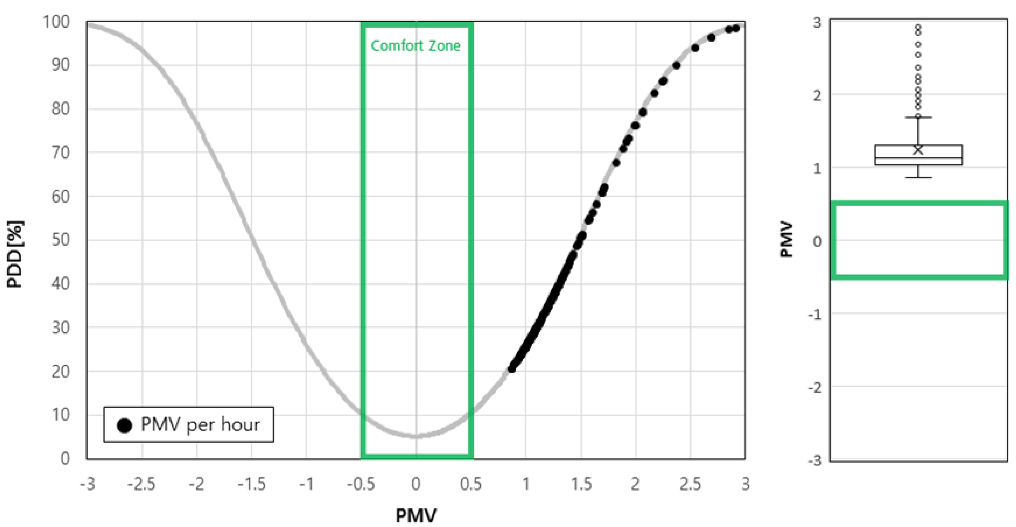
• The comfort hour ratio of the new set-point temperature control was 93.6%, which improved the indoor comfort by 38.5% (26%p) from 67.6% when the MRT was not considered (23 °C set-point temperature control). Consequently, the new set-point temperature considering the thermal characteristics of the building and the weather conditions are regarded to be more effective at improving the indoor comfort than the existing set-point temperature.

The key point of the findings was that the set-point temperature should be modified by each building and the weather conditions, which was verified. In addition to such findings, there are still certain limitations, and future improvements are, therefore, required. Before implementing the method suggested in the present study, an indoor thermal environment dataset of the subject building should be established in advance through simulation modeling. In addition, the derived MRT regression model is limited to a certain building. Thus, the set-point temperature equation derived in this study shows a limitation in terms of the general applicability. In addition, because the thermal comfort is based on multiple thermal components, including the humidity, human activity, and clothing insulation, additional variables should be supported to accurately predict the MRT and should be considered to support the present research findings. Although this study applied the daily set-point temperatures in consideration of the equipment load, hourly intervals’, or other intervals’ set-point temperatures instead of daily set-point temperatures may be more efficient to create a comfortable indoor environment. Future studies will be conducted to derive a set-point temperature equation that can include various thermal-environment factors and the thermal characteristics of buildings based on more diverse data, and calculate hourly set-point temperatures, for which the present study can be applied as basic research. Furthermore, instead of the statistical regression analysis, future studies can consider the state-of-the-art technologies for prediction methods, such as machine learning, artificial intelligence, and ANN, which are widely used throughout the industry, especially by various building researchers [34,36,50,51,52,53]. Considering the trade-off between maintaining indoor comfort and reducing energy consumption, it might be difficult to view the control strategy suggested in this study as a fundamental solution to reduce the energy consumption. Therefore, an HVAC system control that can maintain a high level of indoor comfort and reduce energy consumption in a balanced manner should be developed in future studies.

References

1. Klepeis, N.E.; Nelson, W.C.; Ott, W.R.; Robinson, J.P.; Tsang, A.M.; Switzer, P.; Vbehar, J.; Hern, S.C.; Engelmann, W.H. The National Human Activity Pattern Survey (NHAPS): A resource for assessing exposure to environmental pollutants. J. Expo. Sci. Environ. Epidemiol. 2001, 11, 231–252. [Google Scholar] [CrossRef] [PubMed]
2. Arif, M.; Katafygiotou, M.; Mazroei, A.; Kaushik, A.; Elsarrag, E. Impact of indoor environmental quality on occupant well-being and comfort: A review of the literature. Int. J. Sustain. Built Environ. 2016, 5, 1–11. [Google Scholar]
3. Fanger, P.O. Thermal Comfort. Analysis and Applications in Environmental Engineering; McGrew-Hill: New York, NY, USA, 1972. [Google Scholar]
4. Zhao, R.; Sun, S.; Ding, R. Conditioning strategies of indoor thermal environment in warm climates. Energy Build. 2004, 36, 1281–1286. [Google Scholar] [CrossRef]
5. Barthelmes, V.M.; Becchio, C.; Corgnati, S.P. Occupant behavior lifestyles in a residential nearly zero energy building: Effect on energy use and thermal comfort. Sci. Technol. Built Environ. 2016, 22, 960–975. [Google Scholar] [CrossRef]
6. Jung, J.H. A Proposal of HVAC Control Algorithm Composed of VRF System for Energy Saving and Thermal Comfort in Small-to-Medium Office. Master’s Thesis, Sungkyunkwan University, Suwon, Korea, 2010. [Google Scholar]
7. Montgomery, R.; McDowall, R. Fundamentals of HVAC Control Systems; Elsevier: Burlington, VT, USA, 2008. [Google Scholar]
8. Kim, S.Y. A Proposal of Control Logic for Multi Split Air-conditioner considering Thermal Comfort and Energy Efficiency. Master’s Thesis, Sungkyunkwan University, Suwon, Korea, 2018. [Google Scholar]
9. Freire, R.Z.; Oliveira, G.H.; Mendes, N. Predictive controllers for thermal comfort optimization and energy savings. Energy Build. 2008, 40, 1353–1365. [Google Scholar] [CrossRef]
10. ASHRAE. Standard 55: Thermal Environmental Conditions for Human Occupancy; American Society of Heating Refrigerating and Air-Conditioning Engineers, ASHRAE: Atlanta, GA, USA, 2010. [Google Scholar]
11. Kim, H.G. A study on the Impact of PMV(Predicted Mean Vote) Control on an Office Building Energy Use. Master’s Thesis, Seoul National University, Seoul, Korea, 2009. [Google Scholar]
12. Yun, S.J. A Study on Development of a Simplified PMV Regression Model in an Office Building. Master’s Thesis, University of Seoul, Seoul, Korea, 2013. [Google Scholar]
13. National Law Information Center. Law and Administration Regulations for Guidelines and Suggestions on Air Conditioning and Heating Temperatures for Buildings in Korea. Available online: http://www.law.go.kr (accessed on 21 April 2019).
14. MacArthur, W. Humidity and predicted-mean-vote based(PMV-based) comfort control. ASHRAE Trans. 1986, 92, 5–17. [Google Scholar]
15. Won, J.K. A Study on the Application of Comfort Domain Control in Individual Cooling System for Energy Saving. Master’s Thesis, Sungkyunkwan University, Suwon, Republic of Korea, 2017. [Google Scholar]
16. Castaño-Rosa, R.; Rodríguez-Jiménez, C.; Rubio-Bellido, C. Adaptive thermal comfort potential in mediterranean office buildings: A case study of Torre Sevilla. Sustainability 2018, 10, 3091. [Google Scholar] [CrossRef]
17. ter Mors, S.; Hensen, J.L.; Loomans, M.G.; Boerstra, A.C. Adaptive thermal comfort in primary school classrooms: Creating and validating PMV-based comfort charts. Build. Environ. 2011, 46, 2454–2461. [Google Scholar] [CrossRef] [Green Version]
18. Li, H.; Zhang, Q. Reducing Air-Conditioning System Energy Using a PMV Index. In Proceedings of the Sixth International Conference for Enhanced Building Operations (ICEBO 2006), Shenzhen, China, 6–9 November 2006. [Google Scholar]
19. Jang, H.I.; Suh, S.J. Analysis of indoor thermal environment and energy consumption in office building controlled by PMV. J. Korean Sol. Energy Soc. 2013, 33, 15–22. [Google Scholar] [CrossRef]
20. Liang, J.; Du, R. Thermal comfort control based on neural network for HVAC application. In Proceedings of the IEEE Conference on Control Applications, Toronto, ON, Canada, 28–31 August 2005; pp. 819–824. [Google Scholar]
21. Hamdi, M.; Lachiver, G. A fuzzy control system based on the human sensation of thermal comfort. In Proceedings of the IEEE International Conference on Fuzzy Systems, IEEE World Congress on Computational Intelligence (Cat. No. 98CH36228), Anchorage, AK, USA, 4–9 May 1998; pp. 487–492. [Google Scholar]
22. Yonezawa, K. Comfort air-conditioning control for building energy-saving. In Proceedings of the 26th Annual Conference of the IEEE Industrial Electronics Society (IECON 2000), IEEE International Conference on Industrial Electronics, Control and Instrumentation, 21st Century Technologies, Nagoya, Japan, 22–28 October 2000; pp. 1737–1742. [Google Scholar]
23. Yamada, F.; Yonezawa, K.; Sugawara, S.; Nishimura, N. Development of air-conditioning control algorithm for building energy saving. In Proceedings of the 1999 IEEE International Conference on Control Applications (Cat. No. 99CH36328), Kohala Coast, HI, USA, 22–27 August 1999; pp. 1579–1584. [Google Scholar]
24. Kim, S.H. Development of the PMV Simplification Control Framework for Indoor Thermal Comfort. Ph.D. Thesis, Seoul National University of Science and Technology, Seoul, Korea, 2015. [Google Scholar]
25. Moon, Y.J.; Noh, K.C.; Oh, M.D. Simplification of PMV through multiple regression analysis. Korean J. Air-Cond. Refrig. Eng. 2007, 19, 761–769. [Google Scholar]
26. Kazkaz, M.; Pavelek, M. Operative temperature and globe temperature. Eng. Mech. 2013, 20, 319–325. [Google Scholar]
27. Godbole, S. Investigating the Relationship Between Mean Radiant Temperature (MRT) and Predicted Mean Vote (PMV): A Case Study in a University building. Master’s Thesis, KTH Royal Institute of Technology, Stockholm, Sweden, 2018. [Google Scholar]
28. Chaudhuri, T.; Soh, Y.C.; Bose, S.; Xie, L.; Li, H. On assuming Mean Radiant Temperature equal to air temperature during PMV-based thermal comfort study in air-conditioned buildings. In Proceedings of the IECON 42nd Annual Conference of the IEEE Industrial Electronics Society, Florence, Italy, 23–26 October 2016; pp. 7065–7070. [Google Scholar]
29. Langner, M.; Scherber, K.; Endlicher, W.R. Indoor heat stress: An assessment of human bioclimate using the UTCI in different buildings in Berlin. DIE ERDE J. Geog. Soc. Berl. 2013, 144, 260–273. [Google Scholar]
30. Alfano, F.R.D.A.; Dell’Isola, M.; Palella, B.I.; Riccio, G.; Russi, A. On the measurement of the mean radiant temperature and its influence on the indoor thermal environment assessment. Build. Environ. 2013, 63, 79–88. [Google Scholar] [CrossRef]
31. Kántor, N.; Unger, J. The most problematic variable in the course of human-biometeorological comfort assessment—The mean radiant temperature. Open Geosci. 2011, 3, 90–100. [Google Scholar] [CrossRef]
32. Walikewitz, N.; Jänicke, B.; Langner, M.; Meier, F.; Endlicher, W. The difference between the mean radiant temperature and the air temperature within indoor environments: A case study during summer conditions. Build. Environ. 2015, 84, 151–161. [Google Scholar] [CrossRef]
33. VDI. VDI 3787, Environmental Meteorology. Methods for the Human Biometeorological Evaluation of Climate and Air Quality for Urban and Regional Planning at Regional Level Part 1: Climate; VDI: Düsseldorf, Germany, 2008. [Google Scholar]
34. Na, H.; Choi, J.H.; Kim, H.; Kim, T. Development of a human metabolic rate prediction model based on the use of Kinect-camera generated visual data-driven approaches. Build. Environ. 2019, 160, 106216. [Google Scholar] [CrossRef]
35. Ruiz, I.; Sprowls, M.; Deng, Y.; Kulick, D.; Destaillats, H.; Forzani, E.S. Assessing metabolic rate and indoor air quality with passive environmental sensors. J. Breath Res. 2018, 12, 036012. [Google Scholar] [CrossRef] [PubMed]
36. Ngarambe, J.; Yun, G.Y.; Kim, G. Prediction of indoor clothing insulation levels: A deep learning approach. Energy Build. 2019, 202, 109402. [Google Scholar] [CrossRef]
37. Liu, W.; Yang, D.; Shen, X.; Yang, P. Indoor clothing insulation and thermal history: A clothing model based on logistic function and running mean outdoor temperature. Build. Environ. 2018, 135, 142–152. [Google Scholar] [CrossRef]
38. Korea Meteorological Administration. Weather Information in Republic of Korea. Available online: http://www.weather.go.kr/weather/forecast/timeseries.jsp (accessed on 21 April 2019).
39. Baker, N.; Steemers, K. Energy and Environment in Architecture: A Technical Design Guide; Taylor & Francis: London, UK, 2003. [Google Scholar]
40. Chartered Institute of Building Services Engineers (CIBSE). CIBSE Guide A, Environmental Design; CIBSE: London, UK, 2006. [Google Scholar]
41. ISO. ISO Standard 7730: 2005. Ergonomics of the Thermal Environment-Analytical Determination and Interpretation of Thermal Comfort Using Calculation of the PMV and PPD Indices and Local Thermal Comfort Criteria; ISO: Geneva, Switzerland, 2005. [Google Scholar]
42. ASHRAE. ASHRAE’s Guideline 14-2002 for Measurement of Energy and Demand Savings: How to Determine What was Really Saved by the Retrofit; ASHRAE: Atlanta, GA, USA, 2005. [Google Scholar]
43. ISO. ISO Standard 7726: 1998. Ergonomics of the Thermal Environment-Instruments for Measuring Physical Quantities; ISO: Geneva, Switzerland, 1998. [Google Scholar]
44. Lam, J.C.; Li, D.H.W. Correlation analysis of solar radiation and cloud cover. Int. J. Ambient Energy 1998, 19, 187–198. [Google Scholar] [CrossRef]
45. US Department of Energy. EnergyPlus™ Version 8.6, Documentation Engineering Reference; US Department of Energy: Washington, DC, USA, 2016.
46. US Department of Energy. EnergyPlus™ Version 8.6, Input Output Reference; US Department of Energy: Washington, DC, USA, 2016.
47. Introduction to Correlation and Regression Analysis. Available online: http://sphweb.bumc.bu.edu/otlt/MPH-Modules/BS/BS704_Multivariable/BS704_Multivariable5.html (accessed on 31 July 2019).
48. Multiple Linear Regression Analysis. Available online: http://sphweb.bumc.bu.edu/otlt/MPH-Modules/BS/BS704_Multivariable/BS704_Multivariable7.html (accessed on 31 July 2019).
49. Mason, C.H.; Perreault, W.D., Jr. Collinearity, power, and interpretation of multiple regression analysis. J. Mark. Res. 1991, 28, 268–280. [Google Scholar] [CrossRef]
50. Jang, J.; Baek, J.; Leigh, S.B. Prediction of optimum heating timing based on artificial neural network by utilizing BEMS data. J. Build. Eng. 2019, 22, 66–74. [Google Scholar] [CrossRef]
51. Gonzalez, P.A.; Zamarreno, J.M. Prediction of hourly energy consumption in buildings based on a feedback artificial neural network. Energy Build. 2005, 37, 595–601. [Google Scholar] [CrossRef]
52. Ahmad, M.W.; Mourshed, M.; Rezgui, Y. Trees vs Neurons: Comparison between random forest and ANN for high-resolution prediction of building energy consumption. Energy Build. 2017, 147, 77–89. [Google Scholar] [CrossRef]
53. Valladares, W.; Galindo, M.; Gutierrez, J.; Wu, W.C.; Liao, K.K.; Liao, J.C.; Lu, K.C.; Wang, C.C. Energy optimization associated with thermal comfort and indoor air control via a deep reinforcement learning algorithm. Build. Environ. 2019, 155, 105–117. [Google Scholar] [CrossRef]
Figure 1. Study process.
Sustainability 11 05417 g001
Figure 2. Classification of the subject building floor plan into perimeter and interior zones.
Sustainability 11 05417 g002
Figure 3. (a) Front view of subject building; (b) simulation modeling of subject building.
Sustainability 11 05417 g003
Figure 4. Comparison of electrical energy consumption between actual and simulation modeling of subject floor in August for prediction accuracy.
Sustainability 11 05417 g004
Figure 5. Comparison of MRT regression model for accuracy (controlled at an indoor temperature of 23 °C).
Sustainability 11 05417 g005
Figure 6. Time series plot of calculated set-point temperatures for August.
Sustainability 11 05417 g006
Figure 7. Time series plot of indoor thermal environment data during new set-point temperature control (August 24).
Sustainability 11 05417 g007
Figure 8. Time series plot of indoor temperatures, MRTs, and operative temperatures for August during new set-point temperature control.
Sustainability 11 05417 g008
Figure 9. Distribution of operative temperatures for August during new set-point temperature control.
Sustainability 11 05417 g009
Figure 10. PMV distribution of new set-point temperature control.
Sustainability 11 05417 g010
Figure 11. PMV distribution of 23 ℃ set-point temperature control.
Sustainability 11 05417 g011
Figure 12. PMV distribution of 26 ℃ set-point temperature control.
Sustainability 11 05417 g012