1. Introduction
As the transport system moves toward sustainability, improving the efficiency of the transport system and strengthening the connection of low-carbon modes of transport are becoming important topics. China has underlined a series of key tasks for building national strength in transportation in 2019 [
1]. Conversion from highway to railway and creating a green and efficient modern logistics system are key aspects of sustainable development and low-carbon transport. In this situation, land bridge transportation has gradually reflected its unique advantages regarding sustainability, cost-effectiveness, and reliability in the international supply chain compared with other modes of transport. The Euro–China Expressway, which contributes to the technology, clothing, and food industries, among others, is one typical case of land bridge transport. In its early years, the Euro–China Expressway ran directly from point to point to get a foothold on the transport market share, which has a low actual load rate. From then, it mainly assembled through multimodal hubs to improve efficiency and reduce carbon emissions. The multimodal hubs are international railway stations which undertake the function of road and rail conversion, freight consolidation, and delivery, such as Chongqing in China and Duisburg in Europe. As the recent study shows, transportation is one of the main attributes contributing to the growth of carbon emissions [
2]. Furthermore, road freight transport contributes a large amount of carbon emissions to the total amount of freight-related emissions [
3]. An intermodal road–rail operation would reduce emissions by up to 77.4%, be up to 43.48% more fuel-efficient, and be up to 80% cheaper than operating solely with road transport [
4]. Intermodal routing is eco-friendlier than road-only routing for more than 90% of the simulated shipments in Heinold [
5]. To make progress towards environmental objectives, especially CO
2 emissions, becomes one of the future challenges for transport in Europe [
6]. Therefore, optimizing the consolidation is a key procedure to reduce carbon emissions of the sustainable multimodal transport system.
To achieve sustainable transport, we may decompose the problem into three parts. The first part is to use low carbon transport mode. Rail and maritime play an important role in sustainable transportation. Meanwhile, combined transport provides substantial energy gains and lower CO2 emissions. The second part is to combine location problem with routing problem. It provides a comprehensive transport system solution, which connects to logistics and supply chain. This reflects the optimization of industrial chain resources and aims at economic sustainability. The last part is to reduce carbon emissions as an objective function. This reflects the sustainability of transportation products.
The consolidation of the Euro–China Expressway is a comprehensive transport system that targets the smallest carbon emissions to increase sustainability, which is achieved by utilizing highway and railway modes. This multimodal transport system suffers from multiple problems, including facility locations, international train routes, and vehicle routes. We propose a new problem regarding this transport system, which includes location selection for multimodal stations, international trains schemes, railway routing, and tractor routing. Firstly, the multimodal transport includes highway, domestic railway and international railway systems. These transport systems form a two-echelon network. Secondly, the purpose of the problem is to optimize routing and location, which is a derivative of the location routing problem (LRP). At last, we focus on the consolidation part of the multimodal transport system in the problem. Therefore, in comparison to existing studies, we define this problem as a multimodal transport two-echelon location-routing problem with consolidation (MT-2E-LRP-C).
2. Literature Review
As far as we know, the MT-2E-LRP-C has never been addressed in the literature. However, a series of related problems were studied, including the two-echelon location-routing problem (2E-LRP), the two-echelon vehicle-routing problem (2E-VRP), the tractor and semi-trailer routing problem (TSRP), and the VRP with cross-docking (VRPCD). The abbreviations and full names of related problem in this study are shown in
Table 1.
The location routing problem (LRP) integrates the facility location problem and the path selection of vehicles in the logistics distribution systems. LRP can solve comprehensive problems at the strategic decisions level or at the tactical or operational level (Prodhon [
7]). Earlier studies on LRP by Jacobsen [
8] and Madsen [
9] focused on the distribution of newspapers. Nguyen [
10] first proposed 2E-VRP. Many authors studied 2E-LRP in different variations. Contardo [
11] proposed a two-echelon capacitated location-routing problem (2E-CLRP) with stable capacity of platforms and satellites. Dalfard [
12] considered constraints of vehicle capacity and driving distance based on the model of Contardo. Nguyen [
13] set a 2E-LRP model with a group of vehicles in the central station of the first echelon and a group of sharing vehicles of the second echelon. In particular, the number of vehicles was the decision variable in the model. Different from the above documents, Boccia [
14] focused on the problem with more than one central station of the first echelon, which were called platforms. Fazayeli [
15] aimed to combine the multimodal location-routing problems and time window constraints to maximize customer satisfaction. In 2E-LRP, the potential depot and the route in the first and second echelons should be determined. In our problem, the multimodal stations that serve international train departures, highway routes, and railways will be optimized.
In some logistics problems, particularly at the operational level, the locations of facilities such as stations and satellite sites are determined. Therefore, the location of the 2E-LRP is completed and the 2E-LRP is converted to 2E-VRP. Soysal [
16] focused on a time-dependent 2E-VRP with environmental considerations. Grangier [
17] proposed a two-echelon multiple-trip vehicle-routing problem with satellite synchronization (2E-MTVRP-SS). Li [
18] proposed a two-echelon distribution system considering real-time trans-shipment capacity, varying with trans-shipment and consolidation operations. Kancharla [
19] presented a 2E-VRP model with a different number of vehicles of each vehicle type at each satellite and multi-depot.
The tractor and semi-trailer-routing problem (TSRP), a containerized transportation method for trunk highways (Li [
20]), is a branch research problem that emerged after the truck and trailer routing problem (TTRP). TSRP is the link between road transport and rail container transport. Li [
21] proposed a mixed-integer linear problem (MILP) model and demonstrated that TSRP effectively reduces carbon emissions compared with truck transport. Li [
22] proposed TSRP with many-to-many demand (TSRP-MMD) in an intercity line-haul network setting. In our problem, each highway distribution and multimodal station is visited by several tractors with semi-trailer. The consolidation of the multimodal transport system is completed by tractors with semi-trailers and trains.
The vehicle routing problem with cross-docking was first introduced by Lee [
23]. In VRPCD, freight demand is satisfied by trucks from suppliers’ cross-docking for consolidation prior to customer’s delivery, therefore time-dependent decisions are considered. The sequence of all of the inbound and outbound trucks in the queue influences the efficiency of the cross-docking (Kuo [
24]). Ross [
25], Mousavi [
26], and Seyedhoseini [
27] proposed cross-dock networks where the cross-dock location varied in response to decisions. Ali [
28] proposed the MILP model presented for this problem to increase customer satisfaction by minimizing transportation costs and early/tardy deliveries by scheduling inbound and outbound vehicles. Dondo [
29] studied an N-echelon vehicle-routing problem with cross-docking in supply chain management and dealt with the operational management of hybrid multi-echelon distribution networks. In our problem, there are several similarities with VRPCD, especially the separation of the consolidation and transmission of international trains. The multimodal stations are regarded as cross-docking centers, the multimodal routing is consolidated as pickup routing, and international train routing is considered delivery in VRPCD.
One of the extensions of VRP is VRP with hard time window (VRPHTW). In such models, vehicles visit customers in a limited period of time and early or tardy visits are not permitted (Errico [
30] and Miranda [
31]). Some studies used fuzzy time programming and considered customer satisfaction (Sun [
32]). In our problem, hard time windows are presented in multimodal transport stations.
According to the existing study, we find that these academic issues are getting closer to transport reality. By using the combination of the basic problems of LRP, VRP, TTRP, and TSRP, a two or more echelon network problem will be used. Derived problems, based on different objective functions, various practical scenarios, and a scope of application in different countries and regions, are becoming one of the research hotspots.
Therefore, we propose a MILP model focusing on MT-2E-LRP-C. The objective function is carbon emission of the multimodal transport system. Moreover, a hybrid heuristic algorithm is presented.
3. Problem Description and Formulation
In this section, we propose a multimodal transport two-echelon location-routing problem with consolidation (MT-2E-LRP-C), which aims to minimize the system’s carbon emissions, and give a two-echelon MILP mathematical formulation.
3.1. Problem Description
Our problem focuses on multimodal transport routing and location optimization by using containers. The transport system is composed of several nodes and arcs. A set of nodes V includes domestic multimodal stations , domestic distributions , domestic railway stations , and foreign multimodal stations . Arcs contain a railway route and a highway route. Railway and highway constitute two echelons, which are linked by domestic multimodal stations.
In this network, three sets of demands should be satisfied. The main focus is the consolidation demand, which includes demand between domestic distributions and foreign multimodal stations, and demand between domestic railway stations and foreign multimodal stations. Domestic multimodal stations marshal containers to international railways and dispatch to destinations. Meanwhile, demands between domestic distributions are also considered to promote tractor efficiency and reduce carbon emissions. Therefore, a highway route serves demand between domestic distributions and foreign multimodal stations, and demand between domestic distributions. Supposing that the consolidation is the domestic transport, international transport begins when the trains leave the domestic multimodal stations.
Figure 1 shows an example of this network.
In this multimodal transport network, containers from domestic railway stations are sent to appropriate domestic multimodal stations, such as to , to , and to . Tractors carry the containers from domestic highway distribution centers to other distribution centers and domestic multimodal stations, and finally return to the starting node. Domestic multimodal stations consolidate containers from domestic railway stations and domestic highway distribution centers to international container trains and select appropriate times to send them to foreign multimodal stations.
This problem has the following assumptions:
The containers cannot be separated. The containers are all 40-foot containers.
Tractors’ departure and arrival stations are chosen from one of the multimodal stations.
Demand of highway and multimodal transportation is completely satisfied.
One tractor is served by two drivers to achieve more working hours.
Multimodal stations have no original container demand from other stations. If the demand is needed, we can use a virtual point with demand to solve it.
CO
2 emissions from node transfer operations are negligible, and the emissions produced from routes are considered in several literatures [
33,
34].
The time consumption to attach/detach a container to a tractor in distribution, which is generally considerably short, is not specially considered in the variants of VRP [
35]. Therefore, driver’s working time is equivalent to driving time.
3.2. Notation
(1) Sets
| V | set of nodes, |
| set of domestic multimodal stations |
| set of domestic distributions |
| set of domestic railway stations |
| set of foreign multimodal stations |
| Q | set of tractors, |
| N | set of international trains, |
| set of domestic highway distances between nodes, , |
| set of domestic railway distances between nodes, , |
| set of international railway distance between nodes, , |
| set of demands between domestic distributions, , |
| set of demands between domestic distributions and foreign multimodal stations, , |
| set of demands between domestic railway stations and foreign multimodal stations, , |
| nth () train’s departure time of node to |
(2) Parameters
| velocity of tractor driving alone |
| velocity of tractor driving with semi-trailer |
| velocity of domestic railway |
| velocity of international railway |
| maximum time for a tractor’s route |
| operation time of train in station |
| maximum number of containers for each international train |
| M | arbitrarily large constant |
| carbon emissions of tractor driving 100 kilometers with semi-trailer (kg/100 km) |
| carbon emissions of tractor driving 100 kilometers alone (kg/100 km) |
| carbon emissions of train driving 100 kilometers per container (kg/100 km·container) |
(3) Decision Variables
| If the qth tractor driving alone covers arc , then is 1; otherwise, it is 0. . |
| If the qth tractor driving with a loaded container covers arc , then is 1; otherwise, it is 0. . |
| If the qth tractor departs from , then is 1; otherwise, it is 0. |
| If domestic multimodal station serves demand by the nth train, is 1; otherwise, it is 0. . |
| If domestic multimodal station serves demand by the nth train, is 1; otherwise, it is 0. . |
| . | the nth train which serves is used, is 1; otherwise, it is 0. . |
| Departure time of the qth tractor |
| Arrival time in of the qth tractor |
3.3. Model Formulation
To achieve multimodal transport sustainability, we propose total carbon emissions as the objective function. This is divided into three parts. The first part is the carbon emissions from a highway route by tractors with semi-trailers and tractors driving alone. The second and third parts concern carbon emissions from railway routes by domestic trains and international trains.
Constraints (2)–(11) describe the highway echelon and (12)–(17) describe the railway echelon. Constraint (2) guarantees that tractors keep only one transport condition, which includes driving with a container and driving alone in one arc. Constraint (3) guarantees that tractors leave the origin node without a container. Constraint (4) guarantees that tractors go back to their origin nodes to make a circulation path. Constraint (5) guarantees that each route scheme has only one origin node. Constraint (6) guarantees that routes are continuous. Constraint (7) guarantees that the drivers’ daily maximum working times are satisfied. Constraint (8) guarantees that the demands of the domestic highway stations are satisfied. Constraints (9)–(11) guarantee that the tractors’ departure and arrival times are satisfied. Constraint (12) guarantees that the demands of domestic highway stations to foreign multimodal stations are satisfied. Constraint (13) guarantees that one tractor’s arrival time in a domestic multimodal station is earlier than international railway’s departure time. Constraints (14) and (15) guarantee that the international container flows from highway and railway stations are inseparable. Constraint (16) ensures the maximum number of containers in one international train is satisfied. Constraint (17) defines the variable .
The diesel consumption rates of the most widely used type of container tractor in China are 0.18 L/km and 0.32 L/km for tractors driving alone and tractors driving with semi-trailers. The density of diesel is 0.86 kg/L and the carbon dioxide emission rate of diesel is 3.17 kg/kg of diesel. The carbon dioxide emission of diesel is converted to 2730 g/L. Therefore, we calculate that the values of parameters
and
are 87 kg/100 km and 49 kg/100 km, respectively. Based on calculation method in Sun [
36], we use the up-to-date data from the suitable area in Euro–China Expressway for this model. We can obtain the value of parameter
, which is 12 kg/100 km·container.
4. Solution Method Based on Differential Evolution
In recent studies, differential evolution algorithms efficiently addressed VRP and generated high-quality solutions with strong robustness (Pu [
37] and Küçükoğlu [
38]). Erbao [
39], Cao [
40], and Mingyong [
41] proposed improved differential evolution algorithms and showed that they were effective in solving the open-vehicle-routing problem (OVRP), the vehicle routing problem with fuzzy demands (VRPFD), and the vehicle routing problem with simultaneous pickups and deliveries and time windows (VRP-SPDTW).
The Clarke–Wright savings algorithm (CW algorithm) is easy to implement and has good flexibility and expandability. In addition, the CW algorithm is considered greedy and easily deviates from the optimal solution (Laporte [
42]). Therefore, in many studies, the CW algorithm is used as a construction algorithm for the initial solution (Yanik [
43] and Grasas [
44]).
To solve the comprehensive problems 2E-LRP and 2E-VRP, studies divided them into two sub-problems using a reasonable algorithm (Boccia [
14] and Perboli [
45]). A local search algorithm, which explores different regions of search space to find a local optimum, proved to be a good heuristic algorithm to solve 2E-LRP and 2E-VRP (Hemmelmayr [
46] and Govindan [
47]).
We decompose the problem into two echelons, which include the railway transport echelon and the highway transport echelon as shown in
Table 2. We use a differential evolution algorithm to solve the problem of the railway transport echelon as the main program and we use the CW algorithm and a local search algorithm to solve the problem of the highway echelon.
4.1. Heuristic of Railway Echelon Based on a Differential Evolution Algorithm
We introduce several notations as follows to describe the differential evolution algorithm.
Notation 1. Let K be the number of individuals.
Notation 2. Let G be the number of iterations.
Notation 3. Let denote the set of domestic stations, where the first index specifies the domestic distribution station and the last index specifies the domestic railway station.
Notation 4. Solution representation.
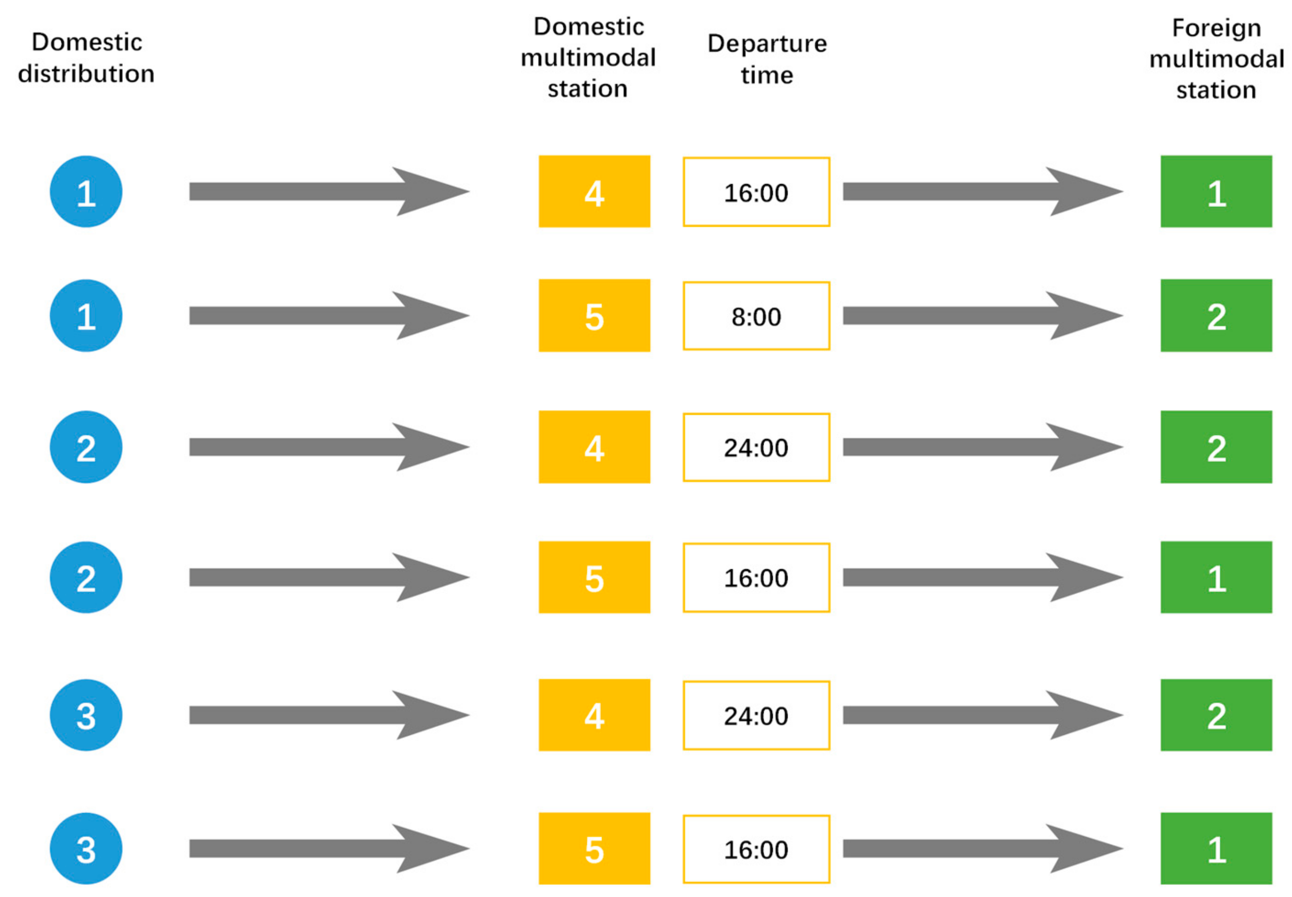
We encode the kth, 1 ≤ k ≤ K, individual in the tth, 1 ≤ t ≤ G, iteration by a -dimension vector . Specifically, represents that the goods required by a foreign multimodal station from a domestic station are transported by the th shift at the domestic multimodal station , in which mod means modular arithmetic in this procedure.
This example represents a 12[(4 + 2)
2]-dimension individual, which includes four domestic distributions, two domestic railway stations, and two foreign multimodal stations.
Figure 2 shows an example of solution representation. There are two domestic multimodal stations with three departure times each. Therefore, the number 4 in the fifth dimension represents that the demands of the first domestic railway station are satisfied by the second domestic multimodal station’s first departure time.
Step 1: Mutation
In the tth generation, each individual , called a target vector, needs to be mutated first. For each , a corresponding mutant vector is generated via the equation , where a, b, c{1,…,K} and a, b, c, k are mutually different. Note that F is a constant, which controls the amplification of the differential variation , and usually takes the value of [0, 2].
Step 2: Rounding
The mutant vector
obtained via the above equation is a real vector. To tackle this situation, a rounding operator is proposed as follows:
This rounding operator always returns the integer within that is closest to .
Step 3: Crossover
Following the mutation and rounding operators, the crossover operation is further applied, in which a trial vector
corresponding to
is generated. The element
is determined by the following equation [
48]:
where
CR [0, 1] is a crossover constant, which needs to be predetermined,
randb(
i) is the
ith evaluation number randomly taken from the uniform distribution [0, 1], and
rnbr(
k) is an integer randomly chosen from the interval
. The condition
i =
rnbr(
k) guarantees that at least one component of the mutant vector is passed to the corresponding trial vector.
4.2. Heuristic of Highway Echelon Based on CW Saving and a Local Search Algorithm
4.2.1. CW Algorithm
The CW saving algorithm combined with the local search algorithm was widely adopted to solve various types of routing problems in the literature (Lai [
49], Zhang [
50], and Li [
51]).
We introduce several notations as follows to describe the CW algorithm.
Notation 1. The matrixes R and are used to denote the set of trips with demands and the set of demands. Let and be the origin and destination of basic trip , where . Let be the demand, where .
Notation 2. Let F be the set of feasible solutions, where .
Notation 3. Let be the update time for the optimal solution and let be the iteration update time.
Our variant of the CW algorithm is implemented as follows:
Step 1: Initialize and transfer matrix to R.
Step 2: Calculate the iteration time. If , go to Step 3. Otherwise, stop and output the solution.
Step 3: Pick a trip randomly and combine other trips in set with an optimal combining selection, which satisfies Constraint (4) and Constraint (9). Choose the trip which has the maximum savings and combine with until new trips can no longer be combined. When there is one combining operation, decreases by 1. Output the route into set F.
Repeat these procedures until . Output the feasible solution F.
Step 4: Calculate the set F. If the objective function is renewed, update the current optimal solution and go to Step 5. Otherwise, go to Step 3.
Step 5: increases by 1. Go to Step 2.
4.2.2. Local Search Algorithm
To improve the objective function generated by the CW algorithm, we use a local search algorithm. According to this MT-2E-LRP-C, four local search operators are used as follows. Each operator has a probability of being selected of 0.25.
(1) Relocate: The operator “relocate” means that two random arcs with loaded containers from one random route can be relocated. After the operation, the quantity of arcs with loaded containers in the route does not change.
(2) Insertion: The operator “insertion” means that one random arc with loaded containers from one random route can be inserted into another random route. After the operation, the first route may be deleted if there is no arc with a loaded container. Therefore, this operation reduces the quantity of tractors from the routing system.
(3) Single swap: The operator “single swap” means that one random arc with loaded containers from one random route can be swapped with one arc from another route. After the operation, the quantity of arcs with loaded containers in the two routes does not change.
(4) Double swap: The operator “double swap” means that two random sequential arcs with loaded containers from one random route can be swapped with two sequential arcs from another route. After the operation, the quantity of arcs with loaded containers in the two routes does not change.
We introduce a notation as follows to describe the local search algorithm.
Notation. Let be the update time for the optimal solution and let be the iteration time.
Step 1: Initialize and let the solution of the CW saving procedure be the initial solution.
Step 2: Calculate the iteration time. If , go to Step 3. Otherwise, stop and output the solution.
Step 3: Select a local search operator and one or two operable routes randomly, execute the operation, and output the feasible solution F.
Step 4: Calculate the set F. If the objective function is renewed, update the current optimal solution and go to Step 5. Otherwise, go to Step 3.
Step 5: increases by 1. Go to Step 2.
5. Computational Experiments
In this section, we generate a series of instances for this problem. The MILP is tested by CPLEX 12.8. The heuristic algorithm is coded in C++ and run on a computer with an Intel(R) Core(TM) i5-6200U 2.3 GHz processor and 8 GB of memory using Windows 10 operating system.
As previous cases of MT-2E-LRP-C utilization have, to our knowledge, not been studied, the model and algorithm are tested on a series of randomly generated instances.
According to realistic multimodal practice, the values of parameters in the model are shown as
Table 3.
5.1. Generation of Instances
(1) Generation of network
We generate three sets of transport distances for the network, which include
,
, and
. According to distances between international railway stations in the Eurasian land bridge,
ranges from 5000 to 14,000 kilometers. In the domestic railway network, in which railway transportation is more competitive with highway transportation,
ranges from 600 to 2000 kilometers. Considering the service ranges of domestic multimodal transport stations and the daily working times of tractors with two drivers,
has three different situations:
(2) Generation of demand
We generate three sets of transport demand, which include , and . Considering the daily service capacity of tractors and the consolidation capacity of stations, ranges from containers, ranges from containers, and ranges from containers.
5.2. Results of Instances
In this section, we discuss a result of a small-scale instance to show the tractor routes and international train schemes. Furthermore, we propose a series of computational results to compare MILP with a heuristic algorithm.
Finally, we propose an example of a multimodal transport route scheme of a instance.
5.2.1. Result of a instance
We generate a instance and display the results, including multimodal transportation consolidation, the railway route, selection of international train departure times, and the highway route.
(1) Network and demand
We generate the set
,
,
,
,
,
randomly as
Table 4.
(2) Result
The objective function is 1.36 × 10
6 kg of carbon dioxide as an optimal cost. There are 27 tractors and four international trains used in this instance. Route of tractors are shown in
Table 5. Route of domestic distributions to foreign multimodal stations and route of railway stations to foreign multimodal stations are shown in
Figure 3 and
Figure 4.
5.2.2. Computational Results of Small-Scale Instances in MILP and a Heuristic Algorithm
We generate five series of instances from different quantities of nodes, including nodes in
,
,
, and
. Moreover, different departure times of international trains are considered. Characteristics of five series of instances is shown in
Table 6.
In the solution process, cplex 12.8 with VS2015 for MILP cannot solve more than two domestic multimodal stations, two foreign multimodal stations, or seven domestic distribution stations in one hour. The results between the MILP and the heuristic algorithm show that the heuristic approach performed well in the solution process, which is shown in
Table 7.
5.2.3. Computational Results of Instances in the Heuristic Algorithm
We generate nine series of different instances solved by the heuristic algorithm. The characteristics of the instances are shown in
Table 8 and
Table 9.
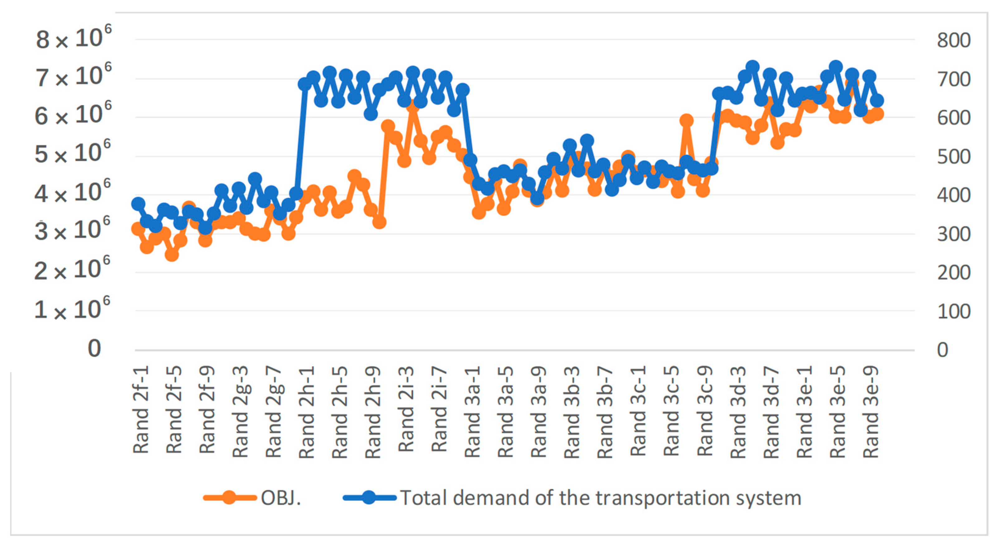
By examining the effect of several parameters on the objective function (OBJ.), we find the quantity of multimodal stations has more impact on carbon emissions in the multimodal transport system, because more multimodal stations lead to more complications for the transportation system.
As shown in
Figure 5 and
Figure 6, container demands of the instances have no strong correlation with carbon emissions.
It is noteworthy that the quantity of tractors has a strong correlation with carbon emissions, as shown in
Figure 7. This result is not noticeable in the realistic multimodal transport practice, so further verification is conducted.
Furthermore, the last nine series of instances are checked (instance Random pc-1 in the following table) and 100 more instances of the
and
(instance Random pc-2 and Random pc-3 in the following table). Pearson correlation, a commonly used test method, has the characteristics of rapid test correlation due to its ability to calculate the covariance and standard deviation of the sequence. It is generally considered that a result above 0.8 represents a strong correlation. We calculate the three series of instances by using Pearson correlation in MATLAB, as
Table 10 shows.
As shown in the three series of instances, the quantity of tractors has a strong correlation with carbon emissions, the objective. The other parameters are unstable. After optimization of this MT-2E-LRP-C, the quantity of tractors reflects the complexity of road collection to a certain extent, and also reflects the significance of consolidation optimization in a multimodal transport system.
6. Case Study
The MT-2E-LRP-C real-world instance is generated from the Euro–China Expressway. As the quantity and frequency of transport using the Euro–China Expressway increases, stations with strong attractive characteristics are appearing. To optimize international train schemes and multimodal transportation routes, we choose a few stations in hinterland cities, including Chengdu, Chongqing, and Xi’an in China and Duisburg, Lodz, and Budapest in Europe. Several distribution centers and railway stations in China are also selected, including Luzhou, Baoji, Qingdao, and Shenzhen, among others.
6.1. Case Description
In this real-world instance, three domestic multimodal stations, three foreign multimodal stations, 10 domestic railway stations, and 20 domestic distributions are chosen and presented in
Table 11.
The real-world instance in
Figure 8 includes the railway echelon and the highway echelon. The two echelons meet at multimodal stations. The railway echelon is the Euro–China Expressway and the highway echelon is composed of the highway in southwestern China. Considering that the demands of the road and the railway in the Euro–China Expressway are hard to measure, the demands of this system are generated randomly.
6.2. Case Computational Results
This real-world instance satisfies demands from 30 railway stations and 60 distribution centers. In order to meet the demand, 615 tractors are selected. The allocation scheme of international trains is shown as follows. The optimization results show that the departure stations and departure times of the Euro–China Expressway are balanced.
The results in
Table 12 show a more comprehensive multimodal transport network than the realistic practice. In this network, each domestic multimodal station has nine international trains for departure, with the quantity of trains in one multimodal station reaching 3000 each year. According to the Chengdu Planning Bureau, the Chengdu Euro–China Expressway, which is the city with the highest quantity of Euro–China trains in China, will reach 3000 in 2035. In the above case study, the result shows an appropriate container allocation scheme for the three domestic multimodal stations. In practice, a reasonable distribution coordination system has not yet been achieved, and irrational competition and subsidies still exist. Furthermore, the Euro–China Expressway is encountering problems concerning containers that are not at their maximum weight load, which is inefficient and leads to excessive carbon emissions. This case study’s consolidation scheme has an average of 33 containers on one international train, which is much more than what we currently see in practice. We also propose a better way to mix the highway and railway containers.
7. Conclusions
In this paper, we refined the practical problems of multimodal transport sustainability and proposed an MT-2E-LRP-C, which is an intercontinental transport dispatching problem. This problem has the characteristics of the general 2E-LRP problem and incorporates aspects of multimodal routing and consolidation. In this paper, a MILP model was established, with the objective function being to lower carbon emissions in the transport system. The decision variables were tractor and railway routes and international train schedules. The time window constraint was set according to the train schedules. We generated a series of random instances and designed a hybrid differential evolution algorithm. We solved the MILP model and the heuristic algorithm for small-scale instances and verified that the MILP model was feasible. The heuristic algorithm had a good solution in terms of its computation time and objective function. Furthermore, we solved the hybrid differential evolution algorithm for large-scale instances and examined the relationships between the demand of multimodal consolidation and carbon emissions, the total demand of a sustainable multimodal transport system and carbon emissions, and the quantity of tractors and carbon emissions. The results show that the overall relationship between demand and carbon emissions is unstable. Moreover, targeted improvement toward tractor efficiency and a reduction in the number of tractors in the sustainable system are important ways of potentially reducing carbon emissions in the system. This conclusion is significant regarding the intercontinental multimodal transportation system, and also provides suggestions regarding the issue of sustainability in the multimodal transportation system. Finally, we conducted an empirical analysis regarding consolidation problems in the Euro–China Expressway. The results show that this problem provides reasonable tractor dispatching, railway routes, and international train schedules.
This study mainly focuses on the statement, modelling and solution method of the MT-2E-LRP-C, which is a segment type comparing with existing articles. We pay more attention to the consolidation part in the multimodal network. The heuristics of DE, CW, and local search algorithms are suitable for the two-echelon problem. The results show that the descriptions of two-echelon and location-routing are meaningful to solve the Euro–China Expressway transport system. Comparing the model results with the transport reality, we find the efficiency of Euro–China Expressway consolidation is still at a lower level. Especially, vicious competition still exists between multimodal stations, which causes the transport to be less sustainable. We suggest that local governments should properly handle competition and cooperation issues in the operation of Euro–China Expressway based on the perspective of sustainable development. Therefore, it will be possible to form a development prospect, including reasonable allocation of station resources, high vehicle efficiency, and high actual load rate of international trains. This study provides new ideas for solving intercontinental sustainable transport problems to some extent. However, a few assumptions and simplified operations can be improved in the further studies to let the problem approach closer to sustainable transport reality. Further study could consider consolidation and delivery links together to obtain more instructive solutions to improve the sustainability of the multimodal transport system.


