Abstract
With China’s commitment to peak its emissions by 2030, sectoral emissions are under the spotlight due to the rolling out of the national emission trading scheme (ETS). However, the current sector policies focus either on the production side or consumption while the majority of sectors along the transmission were overlooked. This research combines input–output modelling and network analysis to track the embodied carbon emissions among thirty sectors of thirty provinces in China. Based on the large-data resolution network, a two-step network reduction algorithm is used to extract the backbone of the network. In addition, network centrality metrics and community detection algorithms are used to assess each individual sector’s roles, and to reveal the carbon communities where sectors have intensive emission links. The research results suggest that the sectors with high out-degree, in-degree or betweenness can act as leverage points for carbon emissions mitigation. In addition to the electricity sector, which is included in the national ETS, the study also found that the metallurgy and construction sectors should be prioritized for emissions reduction from national and local levels. However, the hotpots are different across provinces and thus provincial specific targeted policies should be formed. Moreover, there are nineteen carbon communities in China with different features, which provides direction for provincial governments’ external collaboration for synergistic effects.
1. Introduction
The importance and urgency of reducing sectoral carbon emissions in China is widely recognized [1,2,3,4,5,6]. However, there are many challenges in dealing with the problem efficiently due to the complex supply chain relationships between sectors. For carbon intensive sectors, a large percentage of sectoral outputs are used as intermediate inputs in other sectors of the economy. The intermingled sectoral connections make it challenging to differentiate each sector’s responsibility for carbon emissions and where to target carbon emission reduction strategies.
In the current practice of identifying sector’s responsibilities and advising policy to mitigate emissions, emissions are either allocated completely to the sectors involved in production (the production approach) or completely to those sectors involved in consumption (the consumption approach). The production-based accounting methods prioritize the sectors which directly produce emissions when at source [7,8,9,10]. On the other hand, consumption-based accounting methods attribute all emissions in the supply chain to end use sectors [11,12,13,14]. The argument for adopting a production perspective for the allocation of sectoral carbon emissions include the ease of estimating emissions at the source of emissions. For example, the total carbon emissions for a sector can be directly estimated from the quantity of fossil fuels that are purchased and consumed by a sector, multiplied by known emissions factors for different fuel types. In contrast, when estimating consumption-based emissions, a second step is required that allocates emissions from across the supply chain to final consumers. The argument for using a consumption-based approach is that ultimately it is final consumers who induce demand for goods and services in the economy and thus ultimately it is end users who are responsible for the emissions being produced.
However, both the production perspective and the consumption perspective disregard the transmission of carbon emissions through the economy. While the majority of analysis to date has ignored the transmission perspective, it is beginning to be acknowledged as an important area of investigation [15,16,17]. For example, a transmission perspective can identify the sectors which interact directly with the original source of emissions and the final consumers of end products. The transmission sectors therefore provide a bridge between the producers and consumers and could provide new opportunities for policy development to reduce sectoral carbon emission flows through targeting industrial sectors that are neither responsible for consuming fossil fuels directly from a production perspective nor are they the final consumer of any of these products. By looking into details at the transmission sectors connecting the source of emissions to final consumers, all sectors are put under the microscope and their roles in transmitting carbon through the economy are examined.
This research fills the gap by analyzing data from an environmentally-extended input–output (EE-IOA) table using network analysis to track the embodied carbon emission flows among 30 sectors of 30 provinces in China. An embodied carbon emission network is developed and analyzed using network analysis metrics. More specifically, by examining the roles of sectors through community detection, degree centrality, strength centrality, and betweenness centrality, the carbon intensive communities and hotspots of sectors along the transmission pathway are revealed.
Our research regarding the importance of the transmission perspective is novel and contributes to the literature in the following ways. First, our embodied carbon emission network has a large data resolution, consisting of 30 sectors of 30 provinces, and a two-step network reduction algorithm is adopted to extract the backbone of the network. Therefore, the noise in our network is considerably reduced and the network can reveal the transmission pattern more clearly at a meso level. Secondly, when network metrics is applied to such an adjusted large-resolution network, new insights can be provided. For example, our analysis suggests that the 30 sectors of Beijing are divided into six communities with other province sectors. This structure cannot be identified using other methods where Beijing is taken as a single entity [1,13,18]. Thirdly, our research findings are connected with policy development goals. Specific policies options arising from the findings are proposed at national, provincial and sectoral level.
2. Data
The multi-region input–output (MRIO) table of China in 2012 and sectoral carbon emission data were used to construct the network. The MRIO table covers trade amongst 30 sectors and 30 provinces (excluding Tibet, Taiwan, Hong Kong and Macau due to lack of data) [1]. The carbon emissions from 45 sectors for the year 2012 were calculated using the IPCC sectoral approach, based on energy consumption data and emissions factors from the Chinese statistics bureau [7].
In order to keep sectors consistent between the China MRIO tables and the provincial-level CO2 emission inventory (by IPCC Sectoral Approach), sectors were aggregated. Please see Table A1 in the Appendix A for details on sector matching between the two data bases. After the aggregation, there were 30 sectors and 30 provinces contained in the database.
3. Method
3.1. Network Construction of 2012 Embodied Sectoral Carbon Emissions
The MRIO model tracks flows of products and services among sectors of different regions. The inter-industry production matrix is represented by where element represents the intermediate input from sector (e.g., the metal sector) in region (e.g., Hebei province) to sector (e.g., the construction sector) in region (e.g., Beijing). The final demand vector is represented by , where element represents the amount of products from sector in region sold to final consumers in region . The total output vector is represented by where element is the total output of sector in region . Total output is calculated as the sum of intermediate demand and final demand in the economy as shown by Equation (1).
is defined as technical coefficient matrix, where element is defined as geographical input coefficient. The element is a constant and represents the direct requirement from sector in region per unit of output of sector in region . Formula (1) can be rewritten as
where I is the identity matrix.
Equation (3) is the solution of the basic MRIO model. Given an exogenously specified demand, the equations can be used to calculate the total industrial output directly and indirectly generated by the demand. is the Leontief inverse or total requirements matrix. Each element represents the total amount of products of sector in region that are needed to produce one unit of products of sector in region .
An MRIO-based Chinese economy can be regarded as a network where nodes represent economic sectors, and edges between nodes represent economic transactions between sectors. Carbon emission are transferred along the same economic pathways embodied in goods and services sold through the supply chain. In other words, the carbon emissions that are embodied in the production process of products, are embedded within traded goods or services from one sector to another. These virtual or embodied emissions are transferred from sector i to sector j are represented by the embodied carbon emission transfer network, G in Equation (4). From this notation nodes represent economic sectors and edges between nodes represent the flow of embodied carbon between them.
The embodied carbon emission transfer network of China can be constructed using the following equation.
where k is the carbon emission intensity vector, referring to each sector’s direct production based carbon emission per monetary unit of its total output represented by the units (thousand tons CO2/¥); G is a matrix with the element representing the transfer of embodied carbon emissions from sector in region to sector in region to satisfy the multi-regional final demand . Please note that the elements in the G matrix represent the total embodied emissions within each sector that are both directly and indirectly generated throughout the supply chain. The embodied carbon network is analyzed, and this research presents the final carbon emission transmission relationship among sectors and regions after all rounds of production.
The embodied carbon emission transfer network can be represented by G = (V, E). The set of nodes are defined by V = {(1,1), …, (M,1), (1,2), …, (M,2), …, (1,N), …, (M,N)}, i.e., (industry code, region code). is the adjacent matrix of the network. The set of directed edges is and the carbon emission weights assigned to each edge of the matrix is given by .
3.2. Two-Step Reduction of the Carbon Network
It is difficult to draw information directly from the constructed embodied carbon emission network due to the very large number of non-zero edges contained in the network. Because of the nature of MRIO tables, almost all sector-region pairs are linked by some degree. The redundant intricacy and large number of edges presents challenges for network analysis and the functioning of some network metrics and algorithms. A common way to reduce the number of edges in a network is to set a threshold for edge weight and remove all the edges below the cut-off value.
However, setting the same threshold for all the regions and sectors will downplay the sectors with low carbon emission production, and has very limited noise reduction effect for reducing the statistically insignificant edges connected with the sectors with high carbon emission production. Nonetheless, the sectors with low carbon emission production may potentially be important for carbon emission transmission. In addition, while the edges of high carbon emission production sectors tend to be large in absolute values, some of them are not statistically significant compared with the source sectors’ total emissions. Moreover, the embodied carbon emission network is a strongly disordered network with heavy-tailed statistical distribution of node strength and edge weight. It means that a high percentage of sectors have low carbon emission production and relatively week carbon emission transmission with other sectors. Therefore, it is difficult to set an appropriate threshold value large enough to reduce the number of edges to a manageable size for the network algorithm to function well, and small enough to keep the main structure for sectors with different scales of carbon emission production. For example, a threshold of one ton would reduce 9.5% percent of the total edges, and the noise for high carbon emission production sectors’ edges would be left almost untouched.
In this research, we used Serrano et al.’s [19] algorithm to extract the backbone of the embodied carbon emission network. By using this algorithm, each node was assigned a null model, which informed the random expectation for the distribution of weights associated to its edges, considering the node’s total strength. Each edge was compared with the null model of the two nodes at the end of each edge. Only when an edge was statistically significantly deviant from the null model of at least one of the end nodes, the edge would be kept. The significance level was put at a = 0.05 for this research. By taking the procedure, the nodes with comparatively small strength were not ignored, and the total number of edges were reduced considering all scales in the network.
After the backbone algorithm reduction, we use the threshold of one ton to reduce the network further. If the carbon emission flows between two sectors was less than one ton, the transfer relationship was considered too weak to be included. Therefore, the edge between the two sectors was deleted to further reduce the noise. A total of 92.90% of edges were removed using the backbone algorithm and a further 0.04% of edges were removed using the threshold of 1 ton.
3.3. Community Detection in the Carbon Network
The multi-level modularity optimization algorithm from the R library igraph was adopted to reveal the communities in the embodied carbon emission network. It is a heuristic method based for modularity maximization [20]. This algorithm works well on a large network, especially in terms of computation time and quality measured by modularity. Modularity Q measures the extent to which a network can be grouped into communities with distinct boundaries. It is commonly used to detect unfolding communities in many large networks for a number of different contexts [21,22,23,24].
3.4. Position Measurement of Sectors in the Carbon Network
In this paper, five classic network metrics at node level were adopted to analyze the embodied carbon emission network. Table 1 gives a brief introduction of the metrics. More detailed information about the metrics can be found in Appendix A.2.

Table 1.
Network metrics and its meaning in the context of carbon emission network.
4. Results and Discussions
4.1. Overview of the 2012 Embodied Carbon Emission Network of China
The 2012 embodied carbon emission network was constructed based on the 2012 MRIO table of China. The network had 900 nodes and 774,391 edges. For ease of clear expression, a sector of a province was denoted as a sub-sector, and a sector was denoted the sector at national scale for the following analysis. In the context of the national carbon emission network, there were 900 sub-sectors and therefore 900 nodes in the network. As discussed in Section 3.2, some network metrics cannot function well in a fully connected network. Take the degree centrality for example, 97.11% of all nodes had the same in-degree centrality 876 and out-degree centrality 882. The result was mainly due to the nature of input–output tables, where almost all sectors are connected after all rounds of production are considered. However, some connections are trivial in terms of total embodied emissions. Moreover, there was a large variance for the strength of edges. The maximum edge weight was 82.95 million tons, while the minimum was 0.003 g.
The final network used a backbone algorithm with a coefficient of a = 0.05 and an edge threshold of one ton. The final network therefore only consisted of edges that were statistically significant from the null model (higher than 95%) and with an edge weight that was above one ton. After the two-step network reduction, 886 nodes were retained in the final network. The deletion of 14 nodes were due to the fact that those sub-sector did not produce any carbon emissions and they did not have any significant in-flows and out-flows with other sectors. For example, Shanghai had no coal mining sector and this sector had no significant in-flows and out-flows, so the corresponding node was deleted from the raw network. After completing this process, the number of edges was reduced significantly retaining only 7.0% of all edges and eliminating 719,721 edges. At the same time, 93.0% of the total carbon missions were retained in the final network.
After all insignificant edges were removed, it was easier to extract the relevant information from the network. For an overview of the reduced network, both the degree and edge weight exhibited a long-tail characteristic. Take the degree including both in-degree and out-degree as an example. While the majority of nodes had a total degree of less than 200, there were still quite a few nodes having a much larger degree with a maximum of 921. In addition, the average degree including both in-degree and out-degree was 121. The overall network density was 0.071. (See detailed degree distribution in Figure A1 in the Appendix A).
Figure 1 is a visualization of the 2012 embodied carbon emission network after the two-step reduction process. The figure was drawn by Gephi using the OpenOrd algorithm. The algorithm [25] was good at visualizing a large graph and for revealing both a local and global structure. In the figure below, each node represents a sector within a province and all nodes belonging to the same province were made the same color. The edges among the nodes represent the transmission of embodied emissions between sectors. The color of edges was decided by the source node and all the edges below 100,000 thousand tons were removed to show the transmission pattern more clearly. The sectors with a close trading relationship are graphed by the algorithm to have a close proximity while those with a distant relationship are forced apart. It can be seen that the transmission of embodied carbon emissions is distributed unevenly among the network. In general sectors from the same province have a much closer relationship, because the nodes in the same color tend to be in close proximity. In addition, the provinces in the center of the graph have their sectors highly connected. Especially for some sectors of Beijing, Inner Mongolia, and Jiangsu, which represent the heart of the network and show a close trading relationship with each other. On the other hand, there are some distinguished communities on the periphery of the network, especially for Qinghai and Hainan provinces.
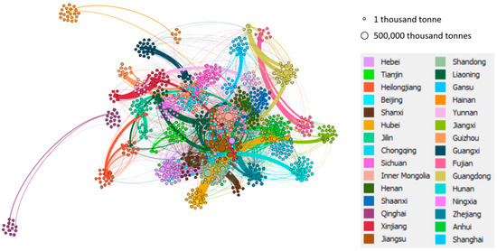
Figure 1.
Visualization of the 2012 embodied carbon emission network.
4.2. Position of Sub-Sectors and Sectors in the 2012 Embodied Carbon Emission Network
4.2.1. Outward Flows
Out-degree and out-strength capture the characteristics of a sector’s outward embodied carbon emission flows. The out-degree metric counts a sector’s export partners, and the sectors with high out-degree centrality are more likely to transmit its emissions to a wide range of other sub-sectors. On the other hand, the out-strength counts the total volume of embodied carbon emissions exported from a sector. Based on the reduced 2012 embodied carbon emission network, out-degree and out-strength for each sub-sector and sector are calculated using the metrics definition in Table 1. See Table 2 below for the summary of the two metrics at sub-sector and sector level. (More details about sector level network metrics can be found in Table A2 in the Appendix A). In addition, out-strength is closely associated with the amount of carbon emissions a sector directly produces. The Spearman correlation between the production-based accounting rank of the sub-sectors and the out-strength rank was 0.94. The high correlation suggested that although carbon intensive sectors produced a large amount of carbon emissions during the production procedure, these carbon-intensive products were mainly used to satisfy the final demand of other sectors.
Table 2.
Summary of out-degree and out-strength metrics. (Unit of out-strength: Thousand tons).
The electricity and hot water production and supply (EWPS) sector had the largest out-degree and out-strength values in every province and at national level. It was mainly due to the fact that the EWPS sector used a very large amount of fossil fuels energy to produce electricity, and electricity was used as inputs almost in all sectors for production. After all rounds of production, those partnerships were strengthened and EWPS sub-sectors ended up with a high out-degree and out-strength centrality.
However, there was a significant mismatch between out-degree rank and out-strength rank for the majority of other sectors. The Spearman correlation between out-degree rank of 900 sub-sectors and out-strength rank was 0.49. (More details about the comparison between out-degree and out-strength rank can be found in Table A3 and Table A4 in Appendix A). This means those sectors are large producers of carbon emissions, but are also below average for transmitting emissions to a wide coverage of other sub-sectors. Take the non-metal product sub-sector as an example. It was listed 23 times in the top 100 high out-strength rank, but only 2 times in the top 100 high out-degree rank. This means that while the non-metal sub-sector is a carbon intensive sector, its products are taken as intermediate inputs by a comparatively small number of other sub-sectors.
Figure 2 shows an example to demonstrate the importance of sectors with a high out-degree. The example in Figure 2 is not intended to draw out sectoral connections in the real economy, but to create a simple five-sector economy for demonstration. Suppose only sector A directly produces carbon emissions e during the whole supply chain. Only sector D, E, and F produce products that are used by final consumers, and they cause carbon emissions at the source by e1, e2, and e3 respectively. From the whole system perspective, the carbon emissions produced at the source should be equal to the carbon emissions caused by final demand, so e = e1 + e2 + e3. The values in brackets are the amount of carbon emissions calculated from a production perspective (left in black) and consumption perspective (right in red).
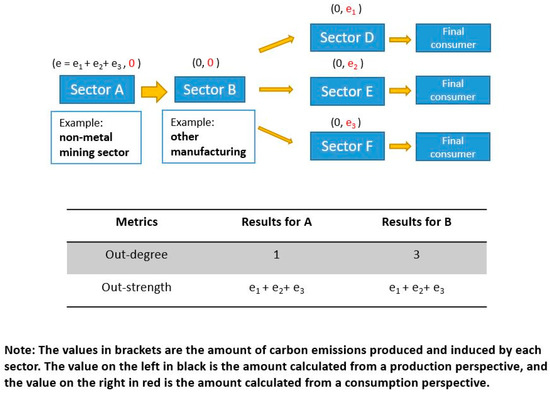
Figure 2.
A five-sector example illustrating the importance of high out-degree sector.
The carbon intensive sector A has a high out-strength, but it does not transmit the carbon emissions to a large coverage of other sectors, which results in low out-degree, such as the non-metal mining sector. It is sector B that spreads out carbon emissions and has a high out-degree, such as “other manufacturing” sector. Sector B is not deemed as important from neither a production or consumption perspectives, but it plays an important role in transmitting the carbon emission out to a wide coverage of other sectors. From a policy perspective, sector B is very important in tracking carbon emissions. By informing the downstream suppliers with carbon information. In time, with relevant policy guidance, it is more likely to bring out the collective efforts of all the downstream players on carbon emission mitigation together.
4.2.2. Inward Flows
In-degree and in-strength capture the characteristics of a sector’s inward embodied carbon emission flows. The in-degree metric counts a sector’s number of import partners, and the sectors with high in-degree centrality are more likely to receive embodied emissions from a wide range of other sub-sectors. On the other hand, the in-strength counts the total volume of embodied carbon emissions imported to a sector. Based on the reduced 2012 embodied carbon emission network, in-degree and in-strength for each sub-sector and sector are calculated using the metric definition in Table 1. See Table 3 below for the summary of the two metrics at sub-sector and sector level. In addition, the Spearman correlation between the in-strength rank of the sub-sectors and the consumption-based accounting rank was 0.96, a very high correlation between the ranks.
Table 3.
Summary of in-degree and in-strength metrics (Unit of in-strength: Thousand tons).
The construction sector had the largest in-degree and in-strength values in every province and at national level. It was mainly because the construction sector uses a large amount of carbon intensive products during the production procedure. In addition, the products of the construction sector, i.e., construction buildings, were mainly used to satisfy final demand. Even though a small percentage of construction buildings were used as intermediate inputs by other sectors, because the sector only produces a small amount of carbon emissions directly and the construction of buildings can be only used locally, the out-strength and out-degree were very small. Therefore, the construction sector can be regarded to be at the end of the value chain.
A mismatch between in-degree rank and in-strength rank for the majority of other sectors can be observed. The Spearman correlation between in-degree rank of 900 sub-sectors and in-strength rank was 0.73. (More details about the comparison between in-degree and in-strength rank can be found in Table A5 and Table A6 in the Appendix A). It suggests that sectors inducing a large amount of carbon emission from consumption perspective were more likely to have high in-degree values. However, there were still some sectors inducing small amount of carbon emissions from consumption perspective had high in-degree values, such as the ‘other manufacturing’ sector of Shanghai with a difference of 335 in the two ranks.
Figure 3 shows an example to demonstrate the importance of sectors with a high in-degree value. Suppose only sector A, B, C produce carbon emissions during the production procedure, and only sector E produces products that are used by final consumers. The carbon intensive sector E has a high in-strength, but it does not receive the carbon emissions from a large range of other sectors, which results in low in-degree, such as the textile sector. It is the sector D that receive carbon emissions from a wide range of sectors and it has a high in-degree, such as transport and storage sector. Sector D is therefore not deemed as important from either a production or consumption perspective, but it plays an important role in transmitting the carbon emission from a wide coverage of sectors. From a policy perspective, sector D is also very important in tracking carbon emissions. By asking for carbon information, sector D is pushing the upstream suppliers to implement carbon tracking practice. In addition, it is good for sector D and the downstream suppliers to make informed decisions to reduce carbon intensive inputs.
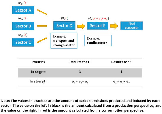
Figure 3.
A five-sector example illustrating the importance of high in-degree sector.
4.2.3. Betweenness
The betweenness of a sub-sector measures its influence as a transmission vehicle for embodied carbon. It examines the amount of embodied carbon emissions going through a sector to satisfy other sectors’ final demand. Sectors with high betweenness are different from carbon emission senders (i.e., out-degree and out-strength) and carbon emission receivers (i.e., in-degree and in-strength). These sectors are in the middle of the supply chain and act purely in a transmission role. Based on the reduced 2012 embodied carbon emission network, betweenness for each sub-sector and sector are calculated using the metric definition in Table 1. See Table 4 below for the summary of this metric at sub-sector and sector level. In addition, metallurgy sector had the largest betweenness value in every province and national level. It suggests that metallurgy takes carbon-intensive inputs from other sub-sectors, and their products are largely used as intermediate inputs for the production of other sub-sectors. (More details about betweenness ranks of sectors and sub-sectors can be found in Table A7 and Table A8 in the Appendix A).
Table 4.
Summary of betweenness values. (Unit: Thousand tons).
Figure 4 shows an example to demonstrate the importance of sectors with high betweenness value. Suppose only six sectors A-F produce carbon emissions during production, and only six sectors J-K produce products that are used by final consumers. In addition, the sum of e1, e2, e3, e4, e5, and e6 is equal to the sum of e7, e8, e9, e10, e11, and e12. In the theoretical situation where sectors G, H, I, J, and K do not produce any emissions and do not sell any products to final consumers, these sectors will be ignored from both a production and consumption perspective. However, these sectors have large betweenness values from a transmission perspective. The betweenness sector focuses on the total amount of carbon emissions going through a sector from a whole economy perspective. In this case, sector I has the largest betweenness value. From a policy perspective, the sectors with high betweenness values can act as a leverage point for collective carbon emission reductions by reducing inputs of carbon-intensive products through production technology improvement. In addition, by supervising and implementing the carbon tracking practice, the sectors with high betweenness and their downstream suppliers can make informed decisions on choosing inputs.
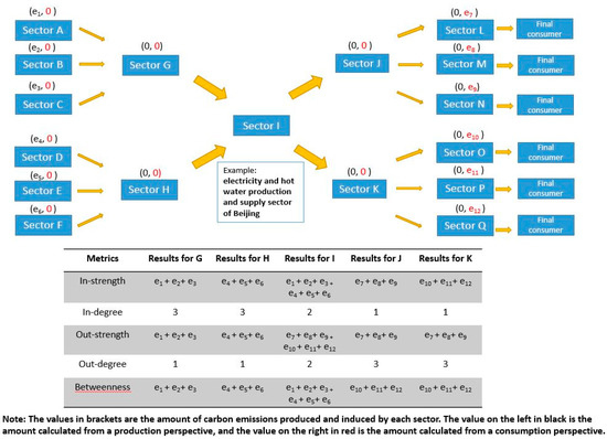
Figure 4.
A simple economy example illustrating the importance of high-betweenness sectors.
The sectors with high betweenness can serve as new acting points for carbon emission mitigation. Take the EWPS (electricity and hot water production and supply) sector of Beijing as an example. From a production perspective, among the EWPS sectors of 30 provinces, Beijing was ranked 27th in terms of direct carbon emission production from high to low. In comparison to other sectors it produced a relatively small amount of carbon emissions and exhibited clean energy characteristics. The carbon emission intensity (carbon emission produced per unit of GDP) was the lowest among all the provinces. From a production perspective, it was not deemed as an urgent sector for carbon emission abatement due to the small amount of carbon emission production and low carbon emission intensity. From a consumption perspective, because it did not induce large amount of carbon emissions from other sectors to satisfy its own final demand, it was not deemed as important either.
However, the EWPS sector of Beijing was identified as having high-betweenness and acted as an intermediary sector within the economy. From a consumption perspective, Beijing-EWPS sector had a comparatively high inflow. The amount of carbon emission transferred from Shanxi-EWPS and Inner-Mongolia-EWPS to Beijing-EWPS was 2.6 times as large as the carbon emission produced by Beijing itself. However, the EWPS was not used to meet final demand of the sector itself. Instead, it was mainly used to meet the final demands of other sectors. The EWPS was used by many other sectors in Beijing, such as the metallurgy sector, and then transferred to many other sectors in other provinces, such as transport equipment in Shanghai. Therefore, there was a comparatively larger amount of embodied carbon emission flows going through Beijing’ EWPS sector, rather than being directly produced or consumed by the sector directly.
4.3. Community of the 2012 Embodied Carbon Emission Network
Nineteen communities of sub-sectors were revealed by using the multi-level modularity optimization algorithm with a modularity score 0.688. The modularity score measures the extent to which a network can be grouped into communities with distinct boundaries [26,27]. It ranges from 0 to 1. The higher the modularity score, the clearer the boundary is. The high modularity score here suggests a fairly distinct boundary among all the communities. Please see Table 5 for the community details. The communities were ranked according to the percentage of the total carbon emission the sectors of a community transmitted were retained within the community (WoT). The carbon flow links among sectors within the community was more intensive than with the sectors outside a community, in terms of both number and weight of edges. In addition, WoT percentage ranged from 49.67% to 96.63%. It suggests that each community exhibited different characteristics. While some communities kept carbon emission flows within its community boundary, other communities had extensive carbon flow connections outside the community.
Table 5.
Communities of the 2012 embodied carbon emission network.
Figure 5 is a visualization of the embodied carbon emission flows among communities using OpenOrd algorithm in Gephi [25]. The nodes represented the communities, and the node size was decided by the within-community carbon emission flows. The edges represented the emission flows transmitted among communities. The color of edges was decided by the source node, the arrows pointed out transmission direction, and the width corresponded to the emission amount. It can be seen that some communities had more intensive interactions than others, which were put in the middle of the network, such as the Jiangsu-Anhui community. Some communities had less interaction, which were put on the periphery of the network, such as Qinghai community. In addition, some communities had significant outflows and inflows with other communities, which can be seen in the large arrows. The significant flows from the Hebei community to the Jiangsu-Anhui community was a good example.
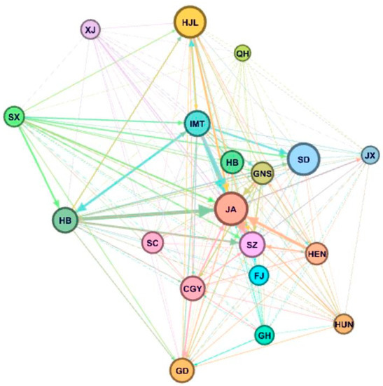
Figure 5.
Visualization of the embodied carbon emission flows among communities in 2012. The community names are abbreviated for visualization purpose in the figure. HB: Hubei community; SC: Sichuan community; SD: Shandong (-Beijing) community; GD: Guangdong community; FJ: Fujian community; QH: Qinghai community; SZ: Shanghai-Zhejiang community; HJL: Heilongjiang-Jilin-Liaoning(-Beijing) community; JA: Jiangsu-Anhui (-Ningxia-Beijing) community; GH: Guangxi-Hainan community; HUN: Hunan community; JX: Jiangxi community; XJ: Xinjiang community; CGY: Chongqing-Guizhou-Yunnan community; HEN: Henan community; GNS: Gansu-Ningxia-Shaanxi community; HB: Hebei(-Beijing) community; IMT: Inner-Mongolia-Tianjin (-Beijing) community; SX: Shanxi(-Beijing) community.
This research identified three community typologies. The first typology included community sectors only belong to one province, and all the sectors of the province were put into this community. Nine communities belonged to this typology, such as Fujian and Jiangxi provinces. In these typologies, the percentage of in-community flow compared to total-flows ranged from 62.8% in the Henan community to 96.6% to Hubei community. They kept the majority of carbon emission flows within their provincial boundary. The second and third typologies included community sub-sectors of more than one province and there were 10 communities belonging to this typology.
The second type of typology, such as the Shanghai-Zhejiang community, had all sectors of the relevant provinces put into one community. The provinces were equally important in terms of the number of sectors put within the community. For the third typology, there was at least one dominant province existing within the community, all of whose sectors were put into the community. The province(s) in a peripheral position had a small number of sectors grouped into the community. Take the Shanxi(-Beijing) community for example. Shanxi province was the dominant province consisting of all 30 sectors. Due to the intensive carbon emission flows between the coal mining sector of Beijing and other sectors of Shanxi, especially considering the large amount of coal mining products directly demanded from Shanxi to Beijing’s coal mining sector, the coal mining sector of Beijing was put into the same community of Shanxi. For the latter two typologies, 8 out of 10 communities kept more than 61.3% of their carbon emissions within the community. However, the Inner Mongolia-Tianjin(-Beijing) community and the Shanxi(-Beijing) community still had extensive carbon emission links outside the communities, with in-community flows out of total flows representing 59.84% and 49.67% respectively.
Thirty sectors of Beijing were separated into six different communities across eleven provinces. This suggests that Beijing is a highly interconnected province. In addition, the amount of imported emissions was much larger than exported emissions. The main reason for this is that Beijing, as the capital of China, is the most developed and populous city in the north, with substantial demand for goods and services from the rest of the economy. While the Beijing has comparatively low production emissions, with the third lowest carbon emissions across all thirty provinces, it consumes a large quantity of carbon intensive products from other areas.
In general, sectors within the same community have a geographically close proximity. This is consistent with the traditional wisdom of regional divisions of China, and at the same time revealed another level of insight. It is common to see six or seven regional division cited in in official sources of China, such as the National Bureau of Statistics of China. Please see Table 3 for details about regional divisions. Provinces in the same region are in close proximity and share similar culture and tend to have higher trading volumes. Duan [28], Zhao [29], and Zhou [30] all used similar regional divisions. This suggests a common assumption from researchers that provinces within regions have intensive carbon emissions exchange.
Our research finds that there is a consistent difference between regional boundaries and the geography of carbon communities. Carbon communities involving multiple provinces are usually formed within a regional boundary. The results showed that there are at least two communities within one region and there is only one community crossing a regional boundary (Inner-Mongolia-Tianjin community). This means that carbon emission flows were not distributed evenly within a region. For the central and north regions, the provinces were comparatively more independent, with each province forming its own community. For other regions, it was common to see two or more provinces put into one community demonstrating a close connection within these provinces. Take East China for example, there were Shanghai-Zhejiang community and Jiangsu-Anhui community. It meant that even though the four provinces were geographically close to each other, the carbon emissions exchange were much more intensive between Shanghai and Zhejiang, and between Jiangsu and Anhui. See more details about the comparison between regional division and community division in Table 6 and Figure 6.
Table 6.
Comparison between region division and community division based on 2012 embodied carbon emission.
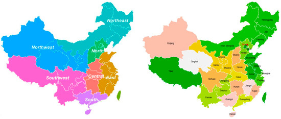
Figure 6.
Comparison between region division and community division based on 2012 embodied carbon emissions. Note: Provinces in the same community was put into the same color.
4.4. Position of Sectors in Carbon Communities
Each community should adopt different priorities for reducing carbon emissions within its sectors, incorporating insights from the outflow, inflow and betweenness perspectives. Despite the fact that EWPS, construction and metallurgy sectors were taken as priority sectors in all communities using outflow, inflow and betweenness perspectives respectively, the majority of the sectors had different roles to play in different carbon communities. Take the outflows in the case of Shanxi community and Hubei community for example. While the coal mining sector, petroleum sector as well as transport and storage sector were sectors with large out-flows, this was not the case in the Hubei community. Instead, food processing and tobacco sector, metal sector, and transport equipment sectors were the large out-flow sectors in Hubei.
There was consistency between community features and sub-sector features. This suggests that localized policies for different communities may provide an alternative policy option. Even for the same metrics, the values vary substantially for each community and therefore require bespoke policies. Looking at out-degree there was significant differences between the top five high out-degree sectors between Shanxi and Hubei communities. In Shanxi community, the out-degree of EWPS sector was 855, and the transport and storage sector was 174, which had the 5th highest out-degree in Shanxi community. In Hubei community, the out-degree of EWPS sector was 147 and the 5th highest out-degree sector, i.e., transport equipment, was 39. This metric result can partly explain the fact that Shanxi community had a comparatively low percentage of in-community flow compared to total-flows, while Hubei community had a high one. In addition, Shanxi province should put more effort in tracking carbon emissions to find out the parties which should be in position to share the responsibility for carbon emission abatement.
5. Conclusions and Policy Implications
Betweenness, out-degree and in-degree provide new information on the transmission pathways within an economy and new opportunities for targeting carbon emission reductions. The EWPS sector in Beijing with a high betweenness metric is one example for targeting carbon mitigation policy. The importance of this sector is missed when using either a production or consumption perspective, but it can act as an important gatekeeper to reduce carbon-intensive inputs for overall carbon emissions reduction. In addition, the low correlation between degree and strength suggests that the sectors which produce or induce large amounts of carbon emissions are not always in a good position to spread or receive emissions from other sectors. Instead, the sectors with high out-degree or in-degree act as a bridge and therefore could serve as new acting point to reduce carbon emissions.
EWPS (electricity and hot water production and supply) sector, construction sector, and metallurgy sector have largest out-flows, in-flows and betweenness flows respectively at provincial, community and national levels. They are important both in the quantity of flows and the number of their sector links. In addition, the EWPS and metallurgy sectors should be given more close attention, because they have large out-flows and betweenness flows at the same time at both local and national levels. However, the majority of sub-sectors had different degree centrality, strength centrality, and betweenness in different communities. Therefore, localized policies should be formed for the same sector in different communities.
Moreover, this analysis highlights the importance of provincial governments in mitigating carbon emissions. Because there are more carbon emissions flows within a community, there may be a synergistic effect if efforts were directed on a carbon community rather than individual sectors. This analysis showed that many communities are formed within the geographical boundary of provinces. This implies that provincial governments have an important role to play in mitigating emissions within their jurisdiction.
Finally, the community detection results provide insights for collaboration among provincial governments tackling the carbon emission mitigation problem together. The discrepancy between the sectors which produce large amount of carbon emissions and the sectors which induce large amount of carbon emissions by consumption asks for collaboration among sectors for dealing with the problem together. The identification of key carbon communities explicitly provides the information about which sub-sectors should be partnered together for effective emissions reduction.
Based on the research results and conclusions, we propose the following policy suggestions. Firstly, the EWPS, metallurgy and construction sector should be prioritized as a focus for carbon emissions reduction from both national and local levels. The recently launched national Emission Trading Scheme (ETS) put the electricity sector as the first priority for carbon mitigation. This is consistent with results from this research which confirms EWPS sector as the top priority for carbon mitigation. The metallurgy sector and construction sector are also important sectors to focus on but have not been on the policy radar yet. In addition, for the majority of sectors, targeted policies should be formed specifically for each different carbon community and local government within a province.
Secondly, carbon emission mitigation policies need to target the sectors with high out-degree, in-degree or betweenness. All three metrics are important for tracing embodied carbon emissions. While the sectors with high out-degree are critical to implementing carbon tracking practice, the sectors with high in-degree are critical for supervising other downstream sectors. The carbon tracking practice can help clarify a sectors’ responsibilities and help governance bodies and companies to make informed decisions to reduce carbon emissions. In addition, for the sectors with high betweenness, which have a large amount of embodied carbon emissions going to these sectors, should focus on reducing the intake of carbon-intensive inputs, which in turn can reduce the carbon emissions at the whole system level. Take the EWPS sector of Beijing as an example, which has high betweenness and out-degree values. For upstream suppliers, the requirement of the carbon tracking information and the preference for low-carbon products, such as wind-generated electricity, can push the upstream sectors to reduce carbon emissions. For the sector itself, it is a key acting point to implement carbon tracking practice to make sure that the carbon emissions are traceable for a large number of downstream suppliers. In this way, the downstream players will be in a better position to collectively work towards carbon emission mitigation by making informed low-carbon purchase decisions.
Thirdly, the community detection results provide direction for provincial governments’ external collaboration and the percentage of in-community flows compared to total-flows suggests the focus for internal improvement or external cooperation. For communities with one province and high percentage of in-community flows compared to total-flows, such as Hubei province, the efforts for carbon emission mitigation would benefit from more internal focus with proposed solutions being the responsibility of individual local governments. For communities consisting of more than one province with high percentage of in-community flows compared to total-flows, close collaboration between the provinces in the same community should be prioritized. Take Shanghai-Zhejiang community for example, the cooperation between the two local governments would yield a synergistic benefit policy benefit. In addition, for communities with comparatively low percentage of in-community flows compared to total-flows, such as Shanxi community, efforts should be made from two directions. While the collaboration within the community should be encouraged, because at least half of carbon emission were kept within the community, the outside links the community has should also be given close attention. In the case of Shanxi community, the strong interactions with Heilongjiang-Jilin-Liaoning community, Hebei community, and Inner-Mongolia-Tianjing also should be considered together for effective emission mitigation.
Finally, Beijing should play roles for the carbon emissions mitigation in China in terms of supervision and knowledge sharing. The fact that the thirty sectors of Beijing were separated into six carbon communities mainly in the north and with a large amount of net imported carbon emission flows requires a strong supervision role with its close trading partners. If Beijing could show clear preference of low-carbon products for both sectors and final demand intakes, it would push the low-carbon transition for the whole northern part of China. In addition, Beijing has the advantage of upgrading low-carbon technology due to an educated workforce. The knowledge sharing between Beijing and the relevant communities would further assist the transition to a low carbon economy.
Author Contributions
Formal analysis, L.H.; Funding acquisition, L.H. and K.L.; Methodology, L.H. and X.L.; Resources, K.L.; Software, X.L.; Supervision, S.K., K.L., X.S. and D.G.; Visualization, L.H.; Writing—original draft, L.H.; Writing—review and editing, S.K., K.L., X.S. and D.G.
Funding
This work was funded by National Natural Science Foundation of China (Grant no. 71774108) and China Scholarship Council (Grant no. 201606890043).
Conflicts of Interest
This manuscript has not been published and is not under consideration for publication elsewhere. We have no conflicts of interest to disclose.
Appendix A
Appendix A.1. Sector Matching between MRIO Tables and Sectoral Carbon Emission Inventory
Table A1.
For sector matching between multi-region input–output (MRIO) tables and sectoral carbon emission inventory.
Table A1.
For sector matching between multi-region input–output (MRIO) tables and sectoral carbon emission inventory.
| Carbon Emission Industries Inventory (Raw) | Carbon Emission Industries Inventory No. (Raw) | Industries No. (Matched) | MRIO No. (Raw) | MRIO (Raw) |
|---|---|---|---|---|
| Farming, Forestry, Animal Husbandry, Fishery and Water Conservancy | 1 | 1 | 1 | Agriculture |
| Coal Mining and Dressing | 2 | 2 | 2 | Coal mining |
| Petroleum and Natural Gas Extraction | 3 | 3 | 3 | Petroleum and gas |
| Ferrous Metals Mining and Dressing | 4 | 4 | 4 | Metal mining |
| Nonferrous Metals Mining and Dressing | 5 | |||
| Nonmetal Minerals Mining and Dressing | 6 | 5 | 5 | Nonmetal mining |
| Other Minerals Mining and Dressing | 7 | |||
| Logging and Transport of Wood and Bamboo | 8 | 6 | 6 | Wood processing and furnishing |
| Timber Processing, Bamboo, Cane, Palm Fiber and Straw Products | 9 | |||
| Furniture Manufacturing | 10 | |||
| Food Processing | 11 | 7 | 7 | Food processing and tobaccos |
| Food Production | 12 | |||
| Beverage Production | 13 | |||
| Tobacco Processing | 14 | |||
| Textile Industry | 15 | 8 | 8 | Textile |
| Garments and Other Fiber Products | 16 | 9 | 9 | Clothing, leather, fur, etc. |
| Leather, Furs, Down and Related Products | 17 | |||
| Papermaking and Paper Products | 18 | 10 | 10 | Paper making, printing, stationery, etc. |
| Printing and Record Medium Reproduction | 19 | |||
| Cultural, Educational and Sports Articles | 20 | |||
| Petroleum Processing and Coking | 21 | 11 | 11 | Petroleum refining, coking, etc. |
| Raw Chemical Materials and Chemical Products | 22 | 12 | 12 | Chemical industry |
| Medical and Pharmaceutical Products | 23 | |||
| Chemical Fiber | 24 | |||
| Rubber Products | 25 | |||
| Plastic Products | 26 | |||
| Nonmetal Mineral Products | 27 | 13 | 13 | Nonmetal products |
| Smelting and Pressing of Ferrous Metals | 28 | 14 | 14 | Metallurgy |
| Smelting and Pressing of Nonferrous Metals | 29 | |||
| Metal Products | 30 | 15 | 15 | Metal products |
| Ordinary Machinery | 31 | 16 | 16 | General and specialist machinery |
| Equipment for Special Purposes | 32 | |||
| Transportation Equipment | 33 | 17 | 17 | Transport equipment |
| Electric Equipment and Machinery | 34 | 18 | 18 | Electrical equipment |
| Electronic and Telecommunications Equipment | 35 | 19 | 19 | Electronic equipment |
| Instruments, Meters, Cultural and Office Machinery | 36 | 20 | 20 | Instrument and meter |
| Other Manufacturing Industry | 37 | 21 | 21 | Other manufacturing |
| Scrap and waste | 38 | |||
| Production and Supply of Electric Power, Steam and Hot Water | 39 | 22 | 22 | Electricity and hot water production and supply |
| Production and Supply of Gas | 40 | 23 | 23 | Gas and water production and supply |
| Production and Supply of Tap Water | 41 | |||
| Construction | 42 | 24 | 24 | Construction |
| Transportation, Storage, Post and Telecommunication Services | 43 | 25 | 25 | Transport and storage |
| Wholesale, Retail Trade and Catering Services | 44 | 26 | 26 | Wholesale and retailing |
| 27 | 27 | Hotel and restaurant | ||
| Others | 45 | 28 | 28 | Leasing and commercial services |
| 29 | 29 | Scientific research | ||
| 30 | 30 | Other services |
Appendix A.2. Network Metrics
Appendix A.2.1. Degree Centrality
Degree centrality captures the connectedness of a node in the network. It measures the importance of a node on counting the number of links the node directly has with other nodes. In a directed network, degree centrality can be categorized into in-degree centrality (number of inbound links) and out-degree centrality (number of outbound links).
In the context of carbon emission network, in-degree centrality measures a sector’s number of import partners, which transferred carbon emissions to this sector. Out-degree centrality measures a sector’s number of export partners, which received carbon emissions from this sector. The sectors with high degree centrality are likely to be in a good position to quickly transfer its emissions to/from other sectors.
The equation for calculating in-degree centrality and out-degree centrality are as follows.
where is the set of nodes connected to node (i, r). If there is an edge from (j, s) to (i, r), = 1, otherwise = 0. If there is an edge from (i, r) to (j, s), = 1, otherwise = 0.
Appendix A.2.2. Strength
Node strength measures the total weights of edges connected to a node. In a directed network, strength is categorized into in-strength and out-strength. In the carbon emission network, in-strength denotes the total volume of embodied carbon emissions imported to a sector. Out-strength denotes the total volume of embodied carbon emissions exported from a sector. The sectors with high strength centrality are likely to produce a large amount of carbon emissions.
The equation for calculating in-degree centrality and out-degree centrality are as follows.
where is the set of nodes connected to node (i, r). is the adjacent matrix of the network. The set of directed edges is E = {(i, r) (j, s)| > 0} and the carbon emissions weight assigned to the edge ((i, r) (j, s)) is .
Appendix A.2.3. Betweenness
The betweenness of one node is defined by the number of shortest paths going through it. Betweenness usually measures the media capability of nodes in the network. If one sector has high betweenness, it means that this sector has strong media capacity. However, this metric is usually based on unweighted and undirected network, and it assumes the connections between nodes happen along with the shortest path [31]. The embodied carbon emission network is a directed and weighted network, and carbon emission flows do not always go along with the shortest path for geographical, economic or historical reason. Therefore, this classic metric algorithm does not function well in the context.
Liang (2016) adjusted the algorithm to better reflect a sector’s media capacity. It considered the direction and weights of input–output network, as well as the weights of nodes’ self-flows. The algorithm calculated the total amount of flows going through a node. Details of the adjusted algorithm can be seen from Liang (2016) paper on betweenness-based method. In the paper, the betweenness of a node bi = fTJiTy, where row vector f is the carbon intensity for each sector’s output, T = LA (A is technology coefficient matrix, and L is Leontief inverse matrix), Ji is a diagonal matrix with all the values on the diagonal equaling to 1, and column vector y is final demand of products from each sectors.
Appendix A.3. Degree Distribution

Figure A1.
Degree distribution of the 2012 reduced embodied carbon emission network.
Appendix A.4. Network Metrics for Sectors at National Level
Table A2.
For network metrics value of sectors at national level.
Table A2.
For network metrics value of sectors at national level.
| Sector | Average Out-Degree | Average Out-Strength | Average In-Degree | Average In-Strength | Average Betweenness | Average Self-Loop | Production Emissions | Consumption Emissions |
|---|---|---|---|---|---|---|---|---|
| Chemical industry | 60.40 | 4756.92 | 49.07 | 8055.66 | 65,239.25 | 1566.38 | 206,390.50 | 317,275.88 |
| Clothing, leather, fur, etc. | 44.73 | 56.80 | 45.97 | 5872.28 | 4643.70 | 200.47 | 7124.48 | 203,643.81 |
| Coal mining | 80.97 | 9570.67 | 25.23 | 896.22 | 20,405.66 | 501.38 | 319,850.76 | 44,813.61 |
| Construction | 29.60 | 38.30 | 347.27 | 98,819.55 | 4331.37 | 2047.81 | 58,307.49 | 3,174,293.51 |
| Electrical equipment | 34.23 | 154.76 | 80.60 | 15,179.85 | 16,995.74 | 257.95 | 11,996.64 | 502,838.24 |
| Electricity and hot water production and supply | 450.43 | 146,000.77 | 39.70 | 2168.37 | 83,872.45 | 16,107.26 | 4,548,789.48 | 556,276.01 |
| Electronic equipment | 32.13 | 66.78 | 63.80 | 7236.20 | 10,923.22 | 163.84 | 6595.64 | 247,003.45 |
| Food processing and tobaccos | 57.13 | 621.81 | 64.03 | 11,482.08 | 16,893.54 | 1182.46 | 55,971.57 | 421,979.86 |
| Gas and water production and supply | 37.20 | 242.51 | 30.00 | 837.78 | 2592.76 | 152.77 | 12,781.76 | 33,066.07 |
| General and specialist machinery | 39.47 | 459.3 | 108.13 | 24,586.45 | 19,551.11 | 1305.95 | 50,371.35 | 836,847.89 |
| Hotel and restaurant | 36.70 | 818.74 | 39.57 | 2808.39 | 5239.45 | 655.32 | 44,953.13 | 115,884.32 |
| Instrument and meter | 32.50 | 17.00 | 38.40 | 1293.28 | 1728.40 | 23.71 | 1178.40 | 45,718.79 |
| Leasing and commercial services | 29.30 | 345.93 | 40.93 | 1194.57 | 6298.45 | 88.27 | 13,776.08 | 44,664.42 |
| Metal mining | 42.67 | 650.90 | 17.57 | 128.04 | 13,276.97 | 12.10 | 21,454.92 | 4315.03 |
| Metal products | 28.90 | 273.99 | 45.63 | 7000.87 | 17,859.51 | 194.17 | 13,869.27 | 241,269.06 |
| Metallurgy | 125.70 | 47,060.83 | 36.23 | 2887.12 | 109,897.99 | 2718.01 | 1,433,169.01 | 179,072.66 |
| Nonmetal mining | 25.40 | 301.90 | 27.90 | 111.57 | 4699.81 | 10.81 | 9700.49 | 4116.60 |
| Nonmetal products | 44.80 | 27,113.44 | 35.70 | 3232.70 | 40,310.77 | 4163.13 | 900,754.84 | 234,073.08 |
| Other manufacturing | 42.77 | 198.78 | 32.53 | 459.38 | 4262.79 | 38.68 | 8327.07 | 17,062.04 |
| Other services | 46.00 | 822.15 | 132.40 | 24,824.28 | 15,369.45 | 2867.98 | 107,908.38 | 912,925.01 |
| Paper making and stationary | 34.80 | 747.68 | 40.40 | 2946.57 | 10,931.34 | 417.63 | 35,801.06 | 113,367.06 |
| Petroleum and gas | 45.93 | 1389.57 | 20.43 | 61.32 | 4062.40 | 54.21 | 52,434.20 | 3734.86 |
| Petroleum refining, coking, etc. | 78.33 | 6721.61 | 39.47 | 1726.34 | 18,747.34 | 870.56 | 249,780.24 | 84,809.07 |
| Scientific research | 23.80 | 80.16 | 51.30 | 2444.44 | 1541.98 | 215.26 | 8294.02 | 92,331.57 |
| Textile | 41.40 | 450.10 | 34.73 | 3659.83 | 12,172.27 | 357.73 | 24,564.82 | 133,715.20 |
| Transport and storage | 91.00 | 13,872.84 | 57.23 | 4947.59 | 22,022.48 | 6207.92 | 616,950.13 | 354,506.71 |
| Transport equipment | 40.40 | 146.40 | 110.73 | 19,756.32 | 14,184.96 | 797.13 | 26,544.96 | 675,957.41 |
| Wholesale and retailing | 44.90 | 1780.72 | 45.77 | 4664.28 | 7409.99 | 1915.97 | 110,141.76 | 216,410.07 |
| Wood processing and furnishing | 30.97 | 119.11 | 41.40 | 2629.64 | 4800.41 | 145.59 | 7637.02 | 95,175.06 |
Appendix A.5. Tables for Comparison of Network Metrics
Table A3.
The frequency of sub-sectors listed in the top 100 sub-sectors in terms of high out-degree and out-strength.
Table A3.
The frequency of sub-sectors listed in the top 100 sub-sectors in terms of high out-degree and out-strength.
| Sector | Out-Degree | Out-Strength |
|---|---|---|
| Electricity and hot water production and supply (EWPS) | 29 | 29 |
| Metallurgy | 19 | 25 |
| Transport and storage | 17 | 11 |
| Coal mining | 10 | 7 |
| Petroleum refining, coking, etc. | 8 | 4 |
| Chemical industry | 6 | 1 |
| Petroleum and gas | 5 | 0 |
| Clothing, leather, fur, etc. | 2 | 0 |
| Nonmetal products | 2 | 23 |
| Agriculture | 1 | 0 |
| Food processing and tobaccos | 1 | 0 |
Table A4.
Out-degree rank and out-strength rank from national sector perspective.
Table A4.
Out-degree rank and out-strength rank from national sector perspective.
| Sector | Out-Degree Rank | Out-Strength Rank | Average Out-Degree | Average Out-Strength | Production Emissions | Consumption Emissions |
|---|---|---|---|---|---|---|
| Electricity and hot water production and supply | 1 | 1 | 450.43 | 146,000.77 | 4,548,789.48 (50.01%) | 556,276.01 (5.48%) |
| Metallurgy | 2 | 2 | 125.70 | 47,060.83 | 1,433,169.01 (15.76%) | 179,072.66 (1.77%) |
| Transport and storage | 3 | 4 | 91.00 | 13,872.84 | 616,950.13 (6.78%) | 354,506.71 (3.50%) |
| Coal mining | 4 | 5 | 80.97 | 9570.67 | 319,850.76 (3.52%) | 44,813.61 (0.44%) |
| Petroleum refining, coking, etc. | 5 | 6 | 78.33 | 6721.61 | 249,780.24 (2.75%) | 84,809.07 (0.84%) |
| Chemical industry | 6 | 7 | 60.40 | 4756.92 | 206,390.50 (2.27%) | 317,275.88 (3.13%) |
| Food processing and tobaccos | 7 | 15 | 57.13 | 621.81 | 55,971.57 (0.62%) | 421,979.86 (4.16%) |
| Other services | 8 | 11 | 46.00 | 822.15 | 107,908.38 (1.19%) | 912,925.01 (9.00%) |
| Petroleum and gas | 9 | 10 | 45.93 | 1389.57 | 52,434.20 (0.58%) | 3734.86 (0.04%) |
| Wholesale and retailing | 10 | 9 | 44.90 | 1780.72 | 110,141.76 (1.21%) | 216,410.07 (2.13%) |
| Nonmetal products | 11 | 3 | 44.80 | 27,113.44 | 900,754.84 (9.90%) | 234,073.08 (2.31%) |
| Clothing, leather, fur, etc. | 12 | 28 | 44.73 | 56.80 | 7124.48 (0.08%) | 203,643.81 (2.01%) |
| Other manufacturing | 13 | 22 | 42.77 | 198.78 | 8327.07 (0.09%) | 17,062.04 (0.17%) |
| Metal mining | 14 | 14 | 42.67 | 650.90 | 21,454.92 (0.24%) | 4315.03 (0.04%) |
| Textile | 15 | 17 | 41.40 | 450.10 | 24,564.82 (0.27%) | 133,715.20 (1.32%) |
| Transport equipment | 16 | 24 | 40.40 | 146.40 | 26,544.96 (0.29%) | 675,957.41 (6.66%) |
| Agriculture | 17 | 8 | 40.23 | 2183.21 | 130,496.03 (1.43%) | 235,704.85 (2.32%) |
| General and specialist machinery | 18 | 16 | 39.47 | 459.30 | 50,371.35 (0.55%) | 836,847.89 (8.25%) |
| Gas and water production and supply | 19 | 21 | 37.20 | 242.51 | 12,781.76 (0.14%) | 33,066.07 (0.33%) |
| Hotel and restaurant | 20 | 12 | 36.70 | 818.74 | 44,953.13 (0.49%) | 115,884.32 (1.14%) |
| Paper making, printing, stationery, etc. | 21 | 13 | 34.80 | 747.68 | 35,801.06 (0.39%) | 113,367.06 (1.12%) |
| Electrical equipment | 22 | 23 | 34.23 | 154.76 | 11,996.64 (0.13%) | 502,838.24 (4.96%) |
| Instrument and meter | 23 | 30 | 32.50 | 17.00 | 1178.40 (0.01%) | 45,718.79 (0.45%) |
| Electronic equipment | 24 | 27 | 32.13 | 66.78 | 6595.64 (0.07%) | 247,003.45 (2.44%) |
| Wood processing and furnishing | 25 | 25 | 30.97 | 119.11 | 7637.02 (0.08%) | 95,175.06 (0.94%) |
| Construction | 26 | 29 | 29.60 | 38.30 | 58,307.49 (0.64%) | 3,174,293.51 (31.30%) |
| Leasing and commercial services | 27 | 18 | 29.30 | 345.93 | 13,776.08 (0.15%) | 44,664.42 (0.44%) |
| Metal products | 28 | 20 | 28.90 | 273.99 | 13,869.27 (0.15%) | 241,269.06 (2.38%) |
| Nonmetal mining | 29 | 19 | 25.40 | 301.90 | 9700.49 (0.11%) | 4116.60 (0.04%) |
| Scientific research | 30 | 26 | 23.80 | 80.16 | 8294.02 (0.09%) | 92,331.57 (0.91%) |
Table A5.
The frequency of sectors listed in the top 100 sectors in in terms of high in-degree and in-strength.
Table A5.
The frequency of sectors listed in the top 100 sectors in in terms of high in-degree and in-strength.
| Row Labels | In-Degree | In-Strength |
|---|---|---|
| Chemical industry | 2 | 3 |
| Clothing, leather, fur, etc. | 3 | 4 |
| Construction | 29 | 29 |
| Electrical equipment | 4 | 7 |
| Electronic equipment | 4 | 2 |
| Food processing and tobaccos | 4 | 5 |
| General and specialist machinery | 11 | 10 |
| Instrument and meter | 0 | 1 |
| Metal products | 3 | 5 |
| Other services | 21 | 19 |
| Paper making, printing & stationery | 1 | 1 |
| Scientific research | 1 | 0 |
| Textile | 1 | 1 |
| Transport and storage | 2 | 0 |
| Transport equipment | 13 | 12 |
| Wholesale and retailing | 1 | 1 |
Table A6.
In-degree rank and In-strength rank from national sector perspective.
Table A6.
In-degree rank and In-strength rank from national sector perspective.
| Row Labels | In-Degree Rank | In-Strength Rank | In-Degree | In-Strength | Production Emissions | Consumption Emissions |
|---|---|---|---|---|---|---|
| Construction | 1 | 1 | 347.27 | 98,819.55 | 58,307.49 (0.64%) | 3,174,293.51 (31.30%) |
| Other services | 2 | 2 | 132.40 | 24,824.28 | 107,908.38 (1.19%) | 912,925.01 (9.00%) |
| Transport equipment | 3 | 4 | 110.73 | 19,756.32 | 26,544.96 (0.29%) | 675,957.41 (6.66%) |
| General and specialist machinery | 4 | 3 | 108.13 | 24,586.45 | 50,371.35 (0.55%) | 836,847.89 (8.25%) |
| Electrical equipment | 5 | 5 | 80.60 | 15,179.85 | 11,996.64 (0.13%) | 502,838.24 (4.96%) |
| Food processing and tobaccos | 6 | 6 | 64.03 | 11,482.08 | 55,971.57 (0.62%) | 421,979.86 (4.16%) |
| Electronic equipment | 7 | 8 | 63.80 | 7236.20 | 6595.64 (0.07%) | 247,003.45 (2.44%) |
| Transport and storage | 8 | 12 | 57.23 | 4947.59 | 616,950.13 (6.78%) | 354,506.71 (3.50%) |
| Scientific research | 9 | 20 | 51.30 | 2444.44 | 8294.02 (0.09%) | 92,331.57 (0.91%) |
| Agriculture | 10 | 11 | 50.67 | 5152.72 | 130,496.03 (1.43%) | 235,704.85 (2.32%) |
| Chemical industry | 11 | 7 | 49.07 | 8055.66 | 206,390.50 (2.27%) | 317,275.88 (3.13%) |
| Clothing, leather, fur, etc. | 12 | 10 | 45.97 | 5872.28 | 7124.48 (0.08%) | 203,643.81 (2.01%) |
| Wholesale and retailing | 13 | 13 | 45.77 | 4664.28 | 110,141.76 (1.21%) | 216,410.07 (2.13%) |
| Metal products | 14 | 9 | 45.63 | 7000.87 | 13,869.27 (0.15%) | 241,269.06 (2.38%) |
| Wood processing and furnishing | 15 | 19 | 41.40 | 2629.64 | 7637.02 (0.08%) | 95,175.06 (0.94%) |
| Leasing and commercial services | 16 | 24 | 40.93 | 1194.57 | 13,776.08 (0.15%) | 44,664.42 (0.44%) |
| Paper making, printing, stationery, etc. | 17 | 16 | 40.40 | 2946.57 | 35,801.06 (0.39%) | 113,367.06 (1.12%) |
| Electricity and hot water production and supply | 18 | 21 | 39.70 | 2168.37 | 4,548,789.48 (50.01%) | 556,276.01 (5.48%) |
| Hotel and restaurant | 19 | 18 | 39.57 | 2808.39 | 44,953.13 (0.49%) | 115,884.32 (1.14%) |
| Petroleum refining, coking, etc. | 20 | 22 | 39.47 | 1726.34 | 249,780.24 (2.75%) | 84,809.07 (0.84%) |
| Instrument and meter | 21 | 23 | 38.40 | 1293.28 | 1178.40 (0.01%) | 45,718.79 (0.45%) |
| Metallurgy | 22 | 17 | 36.23 | 2887.12 | 1,433,169.01 (15.76%) | 179,072.66 (1.77%) |
| Nonmetal products | 23 | 15 | 35.70 | 3232.70 | 900,754.84 (9.90%) | 234,073.08 (2.31%) |
| Textile | 24 | 14 | 34.73 | 3659.83 | 24,564.82 (0.27%) | 133,715.20 (1.32%) |
| Other manufacturing | 25 | 27 | 32.53 | 459.38 | 8327.07 (0.09%) | 17,062.04 (0.17%) |
| Gas and water production and supply | 26 | 26 | 30.00 | 837.78 | 12,781.76 (0.14%) | 33,066.07 (0.33%) |
| Nonmetal mining | 27 | 29 | 27.90 | 111.57 | 9700.49 (0.11%) | 4116.60 (0.04%) |
| Coal mining | 28 | 25 | 25.23 | 896.22 | 319,850.76 (3.52%) | 44,813.61 (0.44%) |
| Petroleum and gas | 29 | 30 | 20.43 | 61.32 | 52,434.20 (0.58%) | 3734.86 (0.04%) |
| Metal mining | 30 | 28 | 17.57 | 128.04 | 21,454.92 (0.24%) | 4315.03 (0.04%) |
Table A7.
The frequency of sectors listed in the top 100 high betweenness sub-sectors.
Table A7.
The frequency of sectors listed in the top 100 high betweenness sub-sectors.
| Sector | Sum of Times | Sum of Betweenness |
|---|---|---|
| Metallurgy | 24 | 3,195,886.66 |
| Electricity and hot water production and supply (EWPS) | 21 | 2,290,397.60 |
| Chemical industry | 13 | 1,558,228.00 |
| Nonmetal products | 11 | 850,299.90 |
| General and specialist machinery | 4 | 350,934.32 |
| Coal mining | 3 | 281,548.00 |
| Electrical equipment | 3 | 260,655.33 |
| Metal products | 3 | 255,348.45 |
| Textile | 3 | 210,511.45 |
| Petroleum refining, coking, etc. | 3 | 196,670.97 |
| Transport and storage | 3 | 161,884.80 |
| Electronic equipment | 2 | 157,179.64 |
| Transport equipment | 2 | 142,936.07 |
| Metal mining | 1 | 120,801.21 |
| Food processing and tobaccos | 2 | 119,357.02 |
| Paper making, printing & stationery | 2 | 105,142.12 |
Table A8.
Betweenness rank from national sector perspective.
Table A8.
Betweenness rank from national sector perspective.
| Sector | Rank | Betweenness | Production Emissions | Consumption Emissions |
|---|---|---|---|---|
| Metallurgy | 1 | 3,296,939.67 | 1,433,169.01 (15.76%) | 179,072.66 (1.77%) |
| Electricity and hot water production and supply | 2 | 2,516,173.47 | 4,548,789.48 (50.01%) | 556,276.01 (5.48%) |
| Chemical industry | 3 | 1,957,177.38 | 206,390.50 (2.27%) | 317,275.88 (3.13%) |
| Nonmetal products | 4 | 1,209,323.13 | 900,754.84 (9.90%) | 234,073.08 (2.31%) |
| Transport and storage | 5 | 660,674.48 | 616,950.13 (6.78%) | 354,506.71 (3.50%) |
| Coal mining | 6 | 612,169.69 | 319,850.76 (3.52%) | 44,813.61 (0.44%) |
| General and specialist machinery | 7 | 586,533.17 | 50,371.35 (0.55%) | 836,847.89 (8.25%) |
| Petroleum refining, coking, etc. | 8 | 562,420.31 | 249,780.24 (2.75%) | 84,809.07 (0.84%) |
| Metal products | 9 | 535,785.36 | 13,869.27 (0.15%) | 241,269.06 (2.38%) |
| Electrical equipment | 10 | 509,872.17 | 11,996.64 (0.13%) | 502,838.24 (4.96%) |
| Food processing and tobaccos | 11 | 506,806.21 | 55,971.57 (0.62%) | 421,979.86 (4.16%) |
| Other services | 12 | 461,083.42 | 107,908.38 (1.19%) | 912,925.01 (9.00%) |
| Transport equipment | 13 | 425,548.66 | 26,544.96 (0.29%) | 675,957.41 (6.66%) |
| Metal mining | 14 | 398,309.01 | 21,454.92 (0.24%) | 4315.03 (0.04%) |
| Textile | 15 | 365,168.00 | 24,564.82 (0.27%) | 133,715.20 (1.32%) |
| Agriculture | 16 | 363,881.14 | 130,496.03 (1.43%) | 235,704.85 (2.32%) |
| Paper making, printing, stationery, etc. | 17 | 327,940.31 | 35,801.06 (0.39%) | 113,367.06 (1.12%) |
| Electronic equipment | 18 | 327,696.49 | 6595.64 (0.07%) | 247,003.45 (2.44%) |
| Wholesale and retailing | 19 | 222,299.72 | 110,141.76 (1.21%) | 216,410.07 (2.13%) |
| Leasing and commercial services | 20 | 188,953.55 | 13,776.08 (0.15%) | 44,664.42 (0.44%) |
| Hotel and restaurant | 21 | 157,183.42 | 44,953.13 (0.49%) | 115,884.32 (1.14%) |
| Wood processing and furnishing | 22 | 144,012.39 | 7637.02 (0.08%) | 95,175.06 (0.94%) |
| Nonmetal mining | 23 | 140,994.22 | 9700.49 (0.11%) | 4116.60 (0.04%) |
| Clothing, leather, fur, etc. | 24 | 139,310.85 | 7124.48 (0.08%) | 203,643.81 (2.01%) |
| Construction | 25 | 129,941.03 | 58,307.49 (0.64%) | 3,174,293.51 (31.30%) |
| Other manufacturing | 26 | 127,883.62 | 8327.07 (0.09%) | 17,062.04 (0.17%) |
| Petroleum and gas | 27 | 121,871.87 | 52,434.20 (0.58%) | 3734.86 (0.04%) |
| Gas and water production and supply | 28 | 77,782.68 | 12,781.76 (0.14%) | 33,066.07 (0.33%) |
| Instrument and meter | 29 | 51,851.99 | 1178.40 (0.01%) | 45,718.79 (0.45%) |
| Scientific research | 30 | 46,259.43 | 8294.02 (0.09%) | 92,331.57 (0.91%) |
References
- Mi, Z.; Meng, J.; Guan, D.; Shan, Y.; Song, M.; Wei, Y.-M.; Liu, Z.; Hubacek, K. Chinese CO2 emission flows have reversed since the global financial crisis. Nat. Commun. 2017, 8, 1712. [Google Scholar] [CrossRef] [PubMed]
- Su, B.; Thomson, E. China’s carbon emissions embodied in (normal and processing) exports and their driving forces, 2006–2012. Energy Econ. 2016, 59, 414–422. [Google Scholar] [CrossRef]
- Zhou, P.; Sun, Z.R.; Zhou, D.Q. Optimal path for controlling CO2 emissions in China: A perspective of efficiency analysis. Energy Econ. 2014, 45, 99–110. [Google Scholar] [CrossRef]
- Andersson, F.N.G. International trade and carbon emissions: The role of Chinese institutional and policy reforms. J. Environ. Manag. 2018, 205, 29–39. [Google Scholar] [CrossRef] [PubMed]
- Wang, X.; Tang, X.; Zhang, B.; McLellan, B.C.; Lv, Y. Provincial carbon emissions reduction allocation plan in China based on consumption perspective. Sustainability 2018, 10, 1342. [Google Scholar] [CrossRef]
- Bai, J.; Qu, J.; Maraseni, T.N.; Wu, J.; Xu, L.; Fan, Y. Spatial and temporal variations of embodied carbon emissions in China’s infrastructure. Sustainability 2019, 11, 749. [Google Scholar] [CrossRef]
- Shan, Y.; Guan, D.; Zheng, H.; Ou, J.; Li, Y.; Meng, J.; Mi, Z.; Liu, Z.; Zhang, Q. China CO2 emission accounts 1997–2015. Sci. Data 2018, 5, 170201. [Google Scholar] [CrossRef]
- Xu, J.H.; Fleiter, T.; Eichhammer, W.; Fan, Y. Energy consumption and CO2 emissions in China’s cement industry: A perspective from LMDI decomposition analysis. Energy Policy 2012, 50, 821–832. [Google Scholar] [CrossRef]
- Lin, B.; Wang, X. Carbon emissions from energy intensive industry in China: Evidence from the iron & steel industry. Renew. Sustain. Energy Rev. 2015, 47, 746–754. [Google Scholar]
- Chen, W.; Wu, F.; Geng, W.; Yu, G. Carbon emissions in China’s industrial sectors. Resour. Conserv. Recycl. 2016, 117, 264–273. [Google Scholar] [CrossRef]
- Su, B.; Ang, B.W. Input-output analysis of CO2 emissions embodied in trade: A multi-region model for China. Appl. Energy 2014, 114, 377–384. [Google Scholar] [CrossRef]
- Liu, L.C.; Liang, Q.M.; Wang, Q. Accounting for China’s regional carbon emissions in 2002 and 2007: Production-based versus consumption-based principles. J. Clean. Prod. 2015, 103, 384–392. [Google Scholar] [CrossRef]
- Meng, L.; Guo, J.; Chai, J.; Zhang, Z. China’s regional CO2 emissions: Characteristics, inter-regional transfer and emission reduction policies. Energy Policy 2011, 39, 6136–6144. [Google Scholar] [CrossRef]
- Zhang, B.; Qiao, H.; Chen, B. Embodied energy uses by China’s four municipalities: A study based on multi-regional input–output model. Ecol. Model. 2015, 318, 138–149. [Google Scholar] [CrossRef]
- Hanaka, T.; Kagawa, S.; Ono, H.; Kanemoto, K. Finding environmentally critical transmission sectors, transactions, and paths in global supply chain networks. Energy Econ. 2017, 68, 44–52. [Google Scholar] [CrossRef]
- Li, Z.; Sun, L.; Geng, Y.; Dong, H.; Ren, J.; Liu, Z.; Tian, X.; Yabar, H.; Higano, Y. Examining industrial structure changes and corresponding carbon emission reduction effect by combining input-output analysis and social network analysis: A comparison study of China and Japan. J. Clean. Prod. 2017, 162, 61–70. [Google Scholar] [CrossRef]
- Liang, S.; Qu, S.; Xu, M. Betweenness-Based Method to Identify Critical Transmission Sectors for Supply Chain Environmental Pressure Mitigation. Environ. Sci. Technol. 2016, 50, 1330–1337. [Google Scholar] [CrossRef]
- Sun, L.; Wang, Q.; Zhou, P.; Cheng, F. Effects of carbon emission transfer on economic spillover and carbon emission reduction in China. J. Clean. Prod. 2016, 112, 1432–1442. [Google Scholar] [CrossRef]
- Serrano, M.Á.; Boguñá, M.; Vespignani, A. Extracting the multiscale backbone of complex. Proc. Natl. Acad. Sci. USA 2009, 106, 6483–6488. [Google Scholar] [CrossRef]
- Blondel, V.D.; Guillaume, J.-L.; Lambiotte, R.; Lefebvre, E. Fast unfolding of communities in large networks. J. Stat. Mech. Theory Exp. 2008, 2008, P10008. [Google Scholar] [CrossRef]
- Del Río-Chanona, R.M.; Grujić, J.; Jensen, H.J. Trends of the world input and output network of global trade. PLoS ONE 2017, 12, 1–15. [Google Scholar] [CrossRef] [PubMed]
- Wagner, A.; Regev, A.; Yosef, N. Revealing the vectors of cellular identity with single-cell genomics. Nat. Biotechnol. 2016, 34, 1145. [Google Scholar] [CrossRef] [PubMed]
- Bassett, D.S.; Wymbs, N.F.; Porter, M.A.; Mucha, P.J.; Carlson, J.M.; Grafton, S.T. Dynamic reconfiguration of human brain networks during learning. Proc. Natl. Acad. Sci. USA 2011, 108, 7641–7646. [Google Scholar] [CrossRef] [PubMed]
- Jia, J.; Li, H.; Zhou, J.; Jiang, M.; Dong, D. Analysis of the transmission characteristics of China’s carbon market transaction price volatility from the perspective of a complex network. Environ. Sci. Pollut. Res. 2018, 25, 7369–7381. [Google Scholar] [CrossRef] [PubMed]
- Martin, S.; Brown, W.M.; Klavans, R.; Boyack, K.W. OpenOrd: An Open-Source Toolbox for Large Graph Layout. In Visualization and Data Analysis 2011; International Society for Optics and Photonics: Bellingham, WA, USA, 2011; Volume 7868, p. 786806. [Google Scholar]
- Chen, C.; Ibekwe-SanJuan, F.; Hou, J. The structure and dynamics of co-citation clusters: A multiple-perspective co-citation analysis. J. Am. Soc. Inf. Sci. Technol. 2010, 61, 1386–1409. [Google Scholar] [CrossRef]
- Martin, J.G., III. Visualizing the Invisible: Application of Knowledge Domain Visualization to the Longstanding Problem of Disciplinary and Professional Conceptualization in Emergency and Disaster Management; Universal-Publishers: Charles Town, MA, USA, 2012; ISBN 1612334288. [Google Scholar]
- Duan, C.; Chen, B.; Feng, K.; Liu, Z.; Hayat, T.; Alsaedi, A.; Ahmad, B. Interregional carbon flows of China. Appl. Energy 2018, 227, 342–352. [Google Scholar] [CrossRef]
- Zhao, Y.; Liu, Y.; Wang, S.; Zhang, Z.; Li, J. Inter-regional linkage analysis of industrial CO2 emissions in China: An application of a hypothetical extraction method. Ecol. Indic. 2015, 61, 428–437. [Google Scholar] [CrossRef]
- Zhou, X.; Zhang, M.; Zhou, M.; Zhou, M. A comparative study on decoupling relationship and influence factors between China’s regional economic development and industrial energy–related carbon emissions. J. Clean. Prod. 2017, 142, 783–800. [Google Scholar] [CrossRef]
- Newman, M. Networks: An introduction; Oxford University Press: Oxford, UK, 2010; ISBN 0199206651. [Google Scholar]
© 2019 by the authors. Licensee MDPI, Basel, Switzerland. This article is an open access article distributed under the terms and conditions of the Creative Commons Attribution (CC BY) license (http://creativecommons.org/licenses/by/4.0/).