4.2. Determination of Sample Size
To ensure the reliability of the model calibration, some simulation data is needed. The ideal sample size is determined using Equation (5):
Including the
N-sample volume,
S is the standard deviation of sample data of observation data, where
S = 8.5 km/h in two lanes,
S = 6.8 km/h in four lanes, and
S = 5.2 km/h in six lanes. The M-normal distribution of the upper probability number when the confidence is 95% (90%) was
m = 1.96 (1.65), and
E is the run error, assuming a speed tolerance of 2–5 km/h. The value of
R satisfies Equation (6).
The object of this study was a two-way, four-lane expressway, and the minimum sample calculation is used as an example. The allowable error was 2 km/h, and this calibration data uses the 85th-percentile average speed, so R = 1.04, and the confidence level was 95%, so m = 1.96. Therefore, the minimum number of samples used to calibrate the road-resistance function was 69.
Because the traffic volume and vehicle type composition were relatively stable in the measured data, the study of the impact of different traffic volumes and different types of vehicles on the road-resistance function had greater limitations. To ensure the diversity of data, this paper used VISSIM simulation software to construct the driving environment under different traffic conditions and different rate of heavy vehicle. In the selection of parameters, the traffic volume was 1950 pcu/h and the minimum traffic volume was 750 pcu/h. With 50 steps, the number of experimental groups was expanded. Therefore, there were 25 simulation experiments under the conditions of each specific rate of heavy vehicle. In this simulation experiment, [2.5%, 32.5%] was divided into equal distances with 2.5% of the ratio of heavy vehicles as the change step, and the simulation experiments are carried out on the proportion of these 13 groups of vehicles.
Sample sizes of different truck ratios under closed half lane and closed inside lane conditions are shown in
Table 3.
It can be seen that each group of tests meets the requirement of minimum sample size 69.
4.3. Significance of Influencing Factors
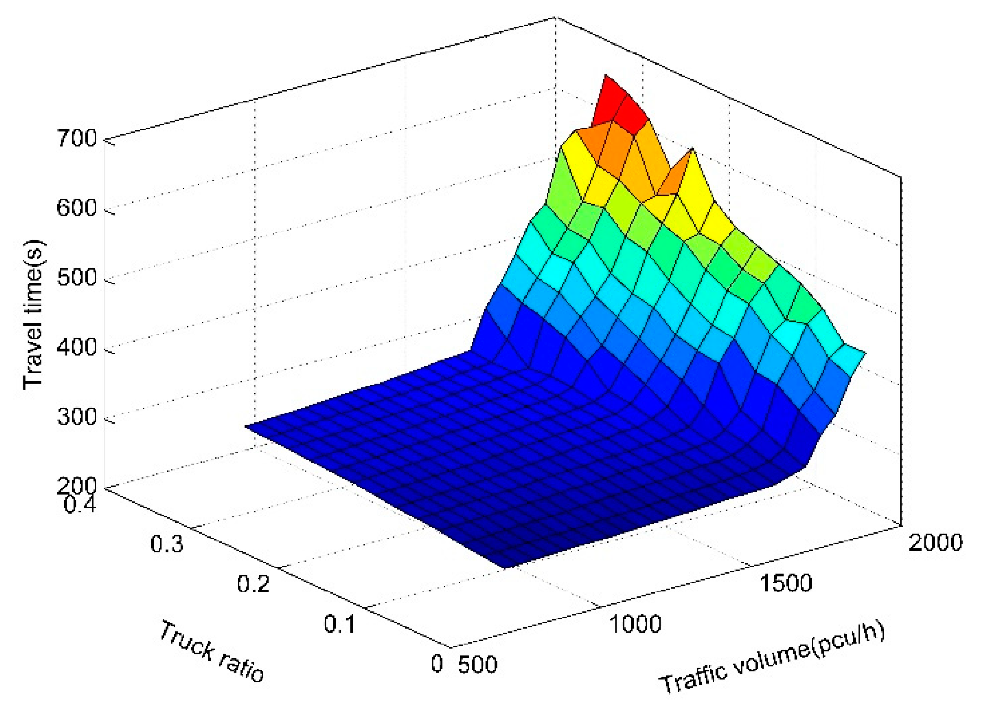
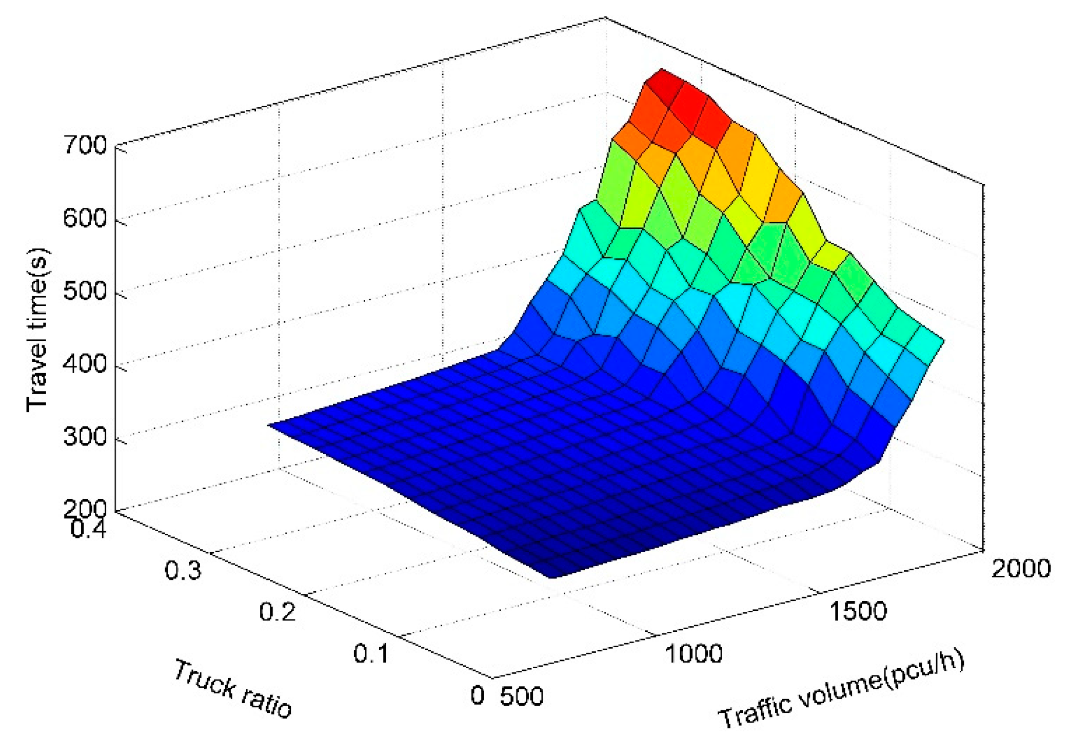
In this simulation experiment, the proportion of models was divided into 13 groups, the traffic volume was divided into 25 groups, and 325 sets of data were simulated under the conditions of closed half-full lanes and enclosed inside lanes, and the travel time of the sections under different conditions was obtained. The simulation results are plotted on a three-dimensional surface, as shown in
Figure 4 and
Figure 5.
From
Figure 4 and
Figure 5, the changes in the travel time are roughly the same in both methods of closing the half-full lane and closing the inside lane. Although the traffic volume and the rate of heavy vehicles were gradually increasing, the change in driving time had the same tendency. Before the critical traffic volume, the trip time increased linearly with the increase of the traffic volume and the rate of heavy vehicles. However, after the critical traffic volume, the travel time increased and the regularity deteriorated; that is, the randomness of the travel time under congestion conditions became stronger. The value of critical traffic volume was greatly affected by the rate of heavy vehicles. Under the condition of closed inside lanes, the critical traffic volume was about 1700 pcu/h in the case of a 10% heavy-vehicle ratio. In the 20% case, the critical traffic volume was about 1650 pcu/h, and in the 30% case, the critical traffic volume was about 1550 pcu/h. That is, as the rate of heavy vehicles increased, the critical traffic volume also decreased. According to this analysis, the average critical traffic volume was 1650 pcu/h. At this time, the expressway was a third-level service, and after the critical traffic volume was greater than the critical traffic volume, it entered a congested state, which is a fourth-level service. After the critical traffic volume, the traffic volume continued to increase, and the travel time increased significantly. At the same time, the rate of heavy vehicles had a significant influence on the travel time. Therefore, after the critical traffic volume was reached, the effect of different vehicle types on traffic diversion was significant.
Before the critical traffic volume, the travel time of the vehicle slowly increased. After the critical traffic volume, the travel time increased rapidly. Using the difference trend as an indicator, the critical traffic under different vehicle types was studied. That is, under the condition of the same heavy vehicle ratio, the critical traffic volumes under the conditions of the closed half-width lane and the closed inside lane were determined, as shown in the
Table 4.
It can be seen that the critical traffic volume for closing the inside or half-width lane did not differ much (
Table 3). In other words, the critical traffic volume was not affected by the closure method but was mainly affected by the rate of heavy vehicles. With the increase in the rate of heavy vehicles, the critical traffic volume gradually increased. Because this study used 50 traffic steps, only a rough estimate of the critical traffic volume could be obtained, which was not accurate. This critical traffic volume can provide suggestions for the essential diversion strategy of the work zone with a speed limit of 60 km/h.
Based on the application of two-way analysis of variance, this paper examined the impact of traffic flow and the rate of heavy vehicle on travel time statistically. It was assumed that the traffic was factor A that influenced the travel time and the vehicle proportion was regarded as the travel time influence factor B. Here, we assumed that the traffic flow and the rate of heavy vehicles were independent of each other and there was no correlation between them. In this paper, 325 sets of simulation data under closed half-lane conditions were used for two-factor analysis with confidence coefficient .
According to calculations, it could be concluded that F
A = 33.474 was much larger than the critical value of 1.75, and F
B = 121.590 was far greater than the critical value of 1.52 (
Table 5). Therefore, both A and B factors should accept the assumption that the flow rate and rate of heavy vehicles had a significant impact on the travel time in the work zone.
4.4. Reasonable Interval of the Rate of Heavy Vehicles
From the above significant test, it can be seen that both the traffic volume and the rate of heavy vehicle had a significant effect on the travel time in the work zone. In the study of the road-resistance function of urban roads, the division of interval for heavy vehicles was at dividing lines of 10%, 20%, and 30% [
21]. However, there is no specific study on the determination of the dividing line. Using the trend difference as a research indicator, the division of interval of the rate of heavy vehicle in the work zone of the highway construction area was studied. The trend difference calculation formula is given as Equation (7):
where
Tj: trend difference in the ratio of j to j;
ti,j: the proportion of vehicles is j, and the traffic volume is the travel time under i simulation conditions;
j: the rate of heavy vehicles;
i: road resistance simulated traffic volume.
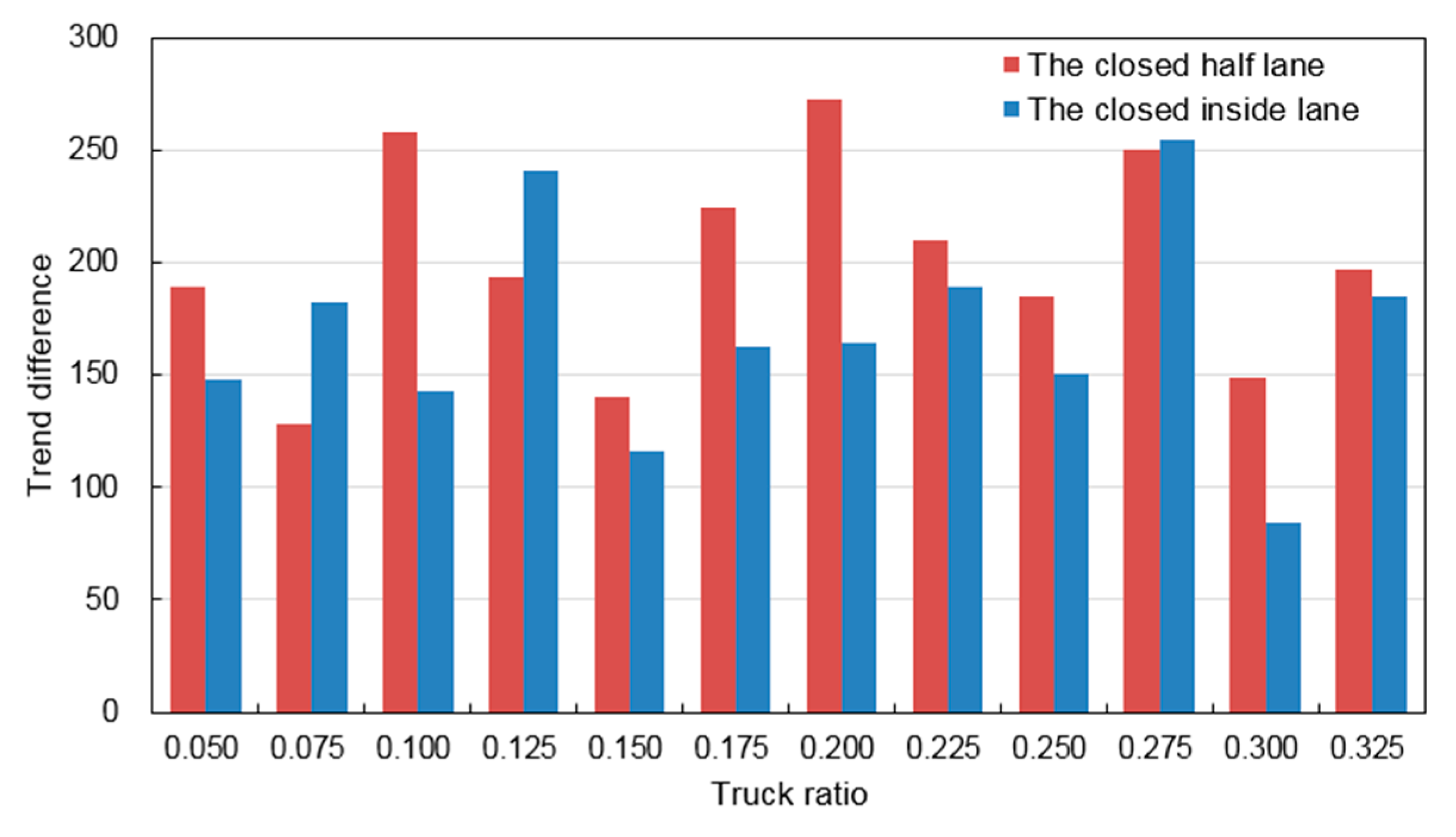
The
Figure 6 is obtained by calculating the trend difference under the two traffic conditions of the enclosed half lane and closed inside lane.
Our results showed that the trend difference in the closed half lane shows a fluctuation such that the minimum difference was 5–7.5%, the maximum difference was 17.5–20%, and the trend of the model proportions of 7.5% and 5% were the closest to no difference (
Figure 4). The difference in trend between the 17.5% and 20% models was the largest. In this study, 250 was used as the critical value of the trend difference. It can be seen that there were three peaks of 10%, 20%, and 27.5% in the model, but the three peak positions were not the criteria for vehicle classification. When the rate of trucks was 10%, there was a crest, indicating that the difference between the 10% and 7.5% cases was large, and it was considered that these two model ratios should have different road-resistance function values. Taking the trend difference of the three wave peaks as the basis for the interval of the rate of trucks, the reasonable interval of the truck ratio in the work zone was divided into
P ≤ 7.5%, 7.5% <
P ≤ 17.5%, 17.5% <
P ≤ 25%, and
P > 25%.
Our results also showed the trend difference under closed inside lane conditions was with a minimum difference of 27.5–30% and a maximum difference of 25–27.5%. The trend of the model proportions of 27.5% and 30% was the closest, with 25% and 27.5% of models having the most significant trend difference. The critical value of the trend difference is 200 under the closed inside lane condition. It can be seen that there were 12.5% and 27.5% peaks in the model proportion. According to the same division method, the model ratio could be divided into P ≤ 10%, 10% < P ≤ 25%, and P > 25%.
4.5. Road-Resistance Functions for Expressway Work Zones
For the BRP function, T, T0, q, c can be obtained from simulation. At this time, the calibration of the BRP function in the construction area is transformed into the calibration of the parameters . The calibration of these parameters can transform the original formula into a parameter-calibration problem.
Set .
The formula is transformed into , and the logarithm of both sides is .
Set .
It was determined that the calibration of and was converted to the parameter-fitting problem of A and B.
A curve-fitting model based on Chebyshev’s meaning in the least-squares method was used.
Take the example of closed inside lane in which
for an introduction and other results were shown in
Table 6. Using the universal global optimization method and the McCourt method in 1stopt, the model parameters
were calibrated. After entering the parameter into 1stopt, after 29 iterations, the model reaches the convergence criterion.
This article uses the mathematical optimization software 1stopt developed by the seven-dimensional high-tech company. Through its unique global optimization algorithm, the optimal solution is finally found as Equation (8).
In the condition of the closed inside lane, the road-resistance function model under the condition that the ratio of trucks is less than 10% is given as Equation (9):
The homogeneity of variance test (F-test) value of the fitted model was F = 396.622. The sample data were used and there were model variables. The critical value of the F test was F
0.05(100,100) = 1.35. It was evident that the F-value was far more significant than the critical value. Because
could not be derived from the look-up table, this paper used Equation (10) to perform the calculations.
, which was much greater than
. Therefore, the goodness-of-fit test results show that the fitting results to the sample data were very good.
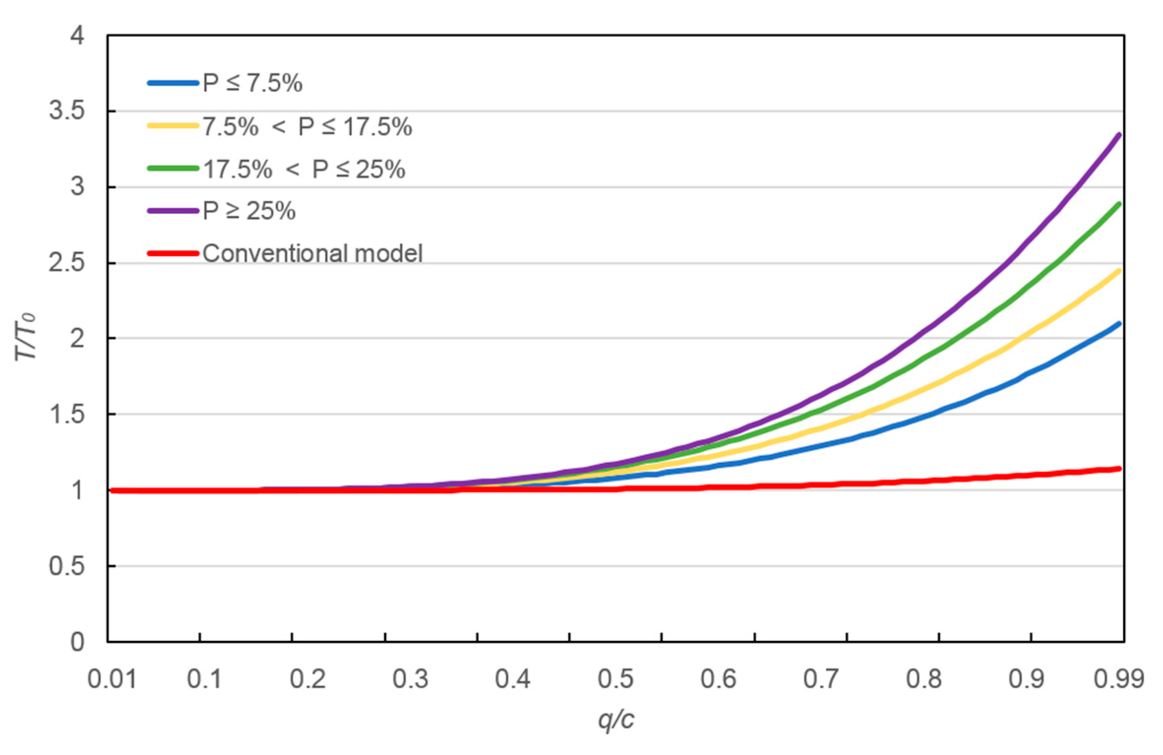
From the
Figure 7, the proposed models and the conventional model began to differ when
q/c equaled 0.3 in the closed inside lane. The proposed models began to differ with different truck ratios when
q/c equaled 0.47 and the difference became larger and larger with the increase of
q/c.
From the
Figure 8, the proposed models and the conventional model began to differ when
q/c equaled 0.25 in the closed half lane. The proposed models began to differ with different truck ratios when
q/c equaled 0.39 and the difference became larger and larger with the increase of
q/c.
It can be seen that the conventional models were very close to the proposed model when q/c was small. Furthermore, the road-resistance function in different truck ratios conditions differed greatly when q/c was large. Therefore, when q/c was large, the proposed models have better adaptability than the conventional model.


