Monitoring of Urban Growth with Improved Model Accuracy by Statistical Methods


Department of Geomatics Engineering, Sivas Cumhuriyet University, 58140 Sivas, Turkey
Sustainability 2019, 11(20), 5579; https://doi.org/10.3390/su11205579
Submission received: 17 September 2019
/
Revised: 7 October 2019
/
Accepted: 7 October 2019
/
Published: 10 October 2019
Abstract
:While the rural population is decreasing day by day, the urban population is increasing rapidly. Urban growth, which occurs as a result of this increase, is sprawling toward natural and environmental areas in urban fringes, and constitutes the main source of many environmental, physical, social, and economic problems. In order to overcome these problems, the direction and rate of urban growth should be determined with simulation models. In this context, many urban growth models have been developed since the 1990s; the SLEUTH urban growth model is one of the most popular among them and has been used in many projects around the world. The brute force calibration process in which the best fit values of growth coefficients are determined is the most important stage of simulation models. The coefficient ranges are initially defined as being between 0 and 100 and are then narrowed in this step according to 13 separate regression scores, which are used to specify the characterization of urban growth. Consensus has not yet been reached as to which metrics should be used for calculating the best fit values, but the Lee–Sallee and Optimum SLEUTH Metric (OSM) methods have been mostly used in past studies. However, in rapidly growing study areas, these methods cannot truly explain urban growth properties. The main purpose of this paper is to precisely calibrate urban growth simulation models. Therefore, Exploratory Factor Analysis (EFA) was used to calculate the growth coefficients, as a new statistical approach for calibration, in this study. The district of Sancaktepe, Istanbul, which experienced population growth of 80% between 2008 and 2018, was selected as the study area in order to test the achievement of the EFA method, and two urban growth simulation models were generated for the years 2030 and 2050. According to the results, despite the fact that there is little effect of urban growth in the short term, more than 70% of forests and agricultural lands are at risk of urbanization by 2050.
1. Introduction
The world population increases every year, and half of this population lives in cities, which offer superior work, education, and health possibilities and a higher level of welfare. This population growth causes urban sprawl as a result of the physical expansion of urban spaces. The main drivers of urban sprawl are defined by the European Environmental Agency (EEA) as macro and micro economic factors, demographic factors, housing preferences, inner city problems, transportation, and regulatory frameworks [1]. Modeling and predicting the direction and speed of urban growth is very important in order to examine the spatio-temporal characteristics of cities for the purposes of smart planning, the efficient use of natural resources, and sustainable development [2]. Probable determinants of urban growth were defined by Liu et al. (2014) for Chinese cities (e.g., land use policy, physical, socio-economic, and neighborhood factors) [3]. If urban growth is not controlled, environmental, social, economic, and physical problems may be faced. According to a report published by the EEA in 2016, the effects of urban growth were discussed under nine titles: land cover, geomorphology, local climate, energy-climate change, air-noise-light pollution, water, flora-fauna, landscape scenery, and land use [4].
Since the second half of the 20th century, the system approach has come to the forefront of planning, and it has been accepted that cities have a dynamic structure consisting of many social, economic, and spatial subsystems with a high level of complexity [5,6,7,8]. Complexity is a characteristic feature of the system, and it may not be predictable in advance [7]. Advanced data mining techniques, which are described as empirical, dynamic, rule-based, agent-based, and machine learning by scientists [9,10,11,12], have been used to analyze the complex structure of urban growth and prevent the problems arising from the expansion of cities.
Data mining tools are divided into two groups, i.e., global parametric and local non-parametric models. While all datasets are used for creating a model in the global parametric approach (e.g., logistic regression, artificial neural networks, genetic algorithms), local non-parametric models (e.g., classification and regression trees, multivariate adaptive regression splines) are generated from partitioned data [13]. Cellular Automata (CA) is the first model that comes to mind among global parametric models for the modeling of complex system behaviors [14] due to its spatial and high computability characteristics. CA is an operating system that is capable of dividing a state into cells and predicting the future state of each cell according to the state of the cells adjacent to it [15].
Although CA is an ideal tool for modeling land use/cover dynamics [16], the modeling achievement of reusing CA is low in some studies, due to pre-defined transition rules [2,17]. Furthermore, while qualitative analyses are investigated in most models, quantitative examinations are ignored [2]. Therefore, determining the true growth characteristics, which has an important impact on land use/cover change prediction models, affects the predictive power of the simulation [2,18]. For this reason, the calibration stage, at which the model validity is tested, plays a key role in the urban growth model, as in all urban CA applications [10,19,20]. As a result, several methods have been developed for model calibration, such as logistic CA with a knowledge-transfer technique [17], that measures the spatio-temporal characteristics of urban growth [2].
In the SLEUTH software, one of the most popular CA-based simulation models developed by Keith C. Clarke, the optimal coefficient values are determined using the Brute Force Calibration (BFC) method [21,22], or genetic algorithms according to 13 criteria [23,24]. In the BFC method, each of the criteria determines the fit between the current state and the model by calculating the least-squares regression values. At the same time, the accuracy of the model is also measured thanks to these regression scores (r2). In the first study of SLEUTH, implemented in the San Francisco Bay area, statistical and visual tests were used to calibrate the model [21]. In the studies carried out to date, model calibrations using different combinations of the 13 Pearson’s r2 values of the urban area emerge [10,14,20,25,26], and the Lee–Sallee parameter is used as a primary metric [8,20,27,28,29,30]. In 2007, Dietzel and Clarke developed a new method for calibration, which they called the Optimum SLEUTH Metric (OSM). In this method, developed by using three different synthetic data, the “compare, population, edges, clusters, slope, x-mean, y-mean” criteria (f-match if land use is modeled) among the 13 parameters of the coupled SLEUTH model are used, and it is claimed that the model calibration yields the most robust results [22].
Although successful models were developed using these methods at the calibration stage, the Lee–Sallee and OSM values were calculated to be very low in some settlement areas where the population growth rate was high and the transportation network geometry had significant effects on urbanization; in such cases, the model parameters did not meet the urbanization characteristics with sufficient accuracy [8,31]. Ayazli (2011) calibrated the model according to the Lee–Salle method while creating a simulation model of the urban growth caused by the third Bosphorus Bridge built in Istanbul using the SLEUTH software [15]. In another study, also conducted in Istanbul, in the model produced according to the OSM method in Sancaktepe district, which had a 55% population increase between 2008 and 2015, calibration values of 17% and below were calculated [31]. In order to establish a more accurate urban growth model, temporal urbanization characteristics should be determined correctly. In this context, Ayazli and Bilen (2019) developed the exploratory factor analysis (EFA) method in order to produce a model with higher accuracy using a new calibration method in which all 13 parameters can be used together at the calibration stage with the BFC method, and intercorrelated parameters are grouped; a model was established using demo data, which is available for download from the Project Gigalopolis website [32].
The aim of this paper is to create an urban growth simulation model with increased accuracy using high spatial resolution data in settlement areas with high urbanization rates. Unfortunately, calibration values are not always at the desired level in models calibrated by the OSM and Lee–Sallee methods. It is necessary to decide which metrics will be used by considering the urbanization characteristics in the model calibration. Expert opinions are naturally important at this stage; however, being able to perform this selection objectively by a statistical method will also protect the model from subjective errors that may occur due to expert opinions. Therefore, it was considered appropriate to use the EFA method, a new statistical approach, in this study for the SLEUTH model calibration. According to the EFA method, intercorrelated metrics are grouped in order to ensure the use of the highest possible number of criteria in calibration, according to the obtained weighted factor scores. In this context, the answers to the following questions were sought in this paper:
- Which calibration method should be used to increase the accuracy of SLEUTH urban growth simulation models created using high-resolution data in settlement areas with high population growth?
- What is the success of the EFA method in an urban growth simulation model calibrated using real data?
- Can the EFA method serve as an alternative in simulation studies in which the OSM and Lee–Sallee scores are calculated to be low?
- What will be the change in land cover in settlements with rapid population growth according to the high-resolution simulation model calibrated by the EFA method?
Sancaktepe district, which was established in Istanbul in 2008 as a result of combining three different towns, and in which urban growth intensely threatens agricultural lands and forest areas, was selected as the study area. Although the projected population was 333,174 in the masterplan prepared in 2010, the population of the district increased by 81% between 2008 and 2018, reaching 414,143 [33]. Rapid population growth and rent-oriented political decisions triggered urban growth, which leads to land use/cover change in the urban fringe. Therefore, monitoring the urban growth of Sancaktepe and determining the land cover change there are the aims of this paper.
At the beginning of this study, four different time periods were determined: 1961, 1992, 2001, and 2014. Changes occurring in land cover since 1961, i.e., for more than 50 years, were examined, and a CA-based simulation model for the years 2030 and 2050 was established. Since the calibration values of the models created according to the OSM and Lee–Sallee methods were low in the study area [34,35], it became necessary to use a new calibration method in the simulation model to be created for Sancaktepe. As a result, thanks to the EFA method, a model was obtained in which all the metrics were used in different weights at the calibration stage.
The paper is organized into four sections. In the Introduction, the aim of the study, the methods and data used, and previous studies in the literature are discussed. The data used in the study, the characteristics of CA-based urban growth simulation models, the working principles of the SLEUTH software, the Lee–Sallee criterion, and the model calibration by the OSM and EFA methods are discussed in the Methodology section. The obtained results are presented comparatively in the Results section, and the paper is concluded with a Discussion and Conclusions section, in which the results are discussed.
2. Methodology
2.1. Creation of a Simulation Model Using SLEUTH
The parameters required for the SLEUTH software, which was developed by Dr. Keith C. Clarke at the Department of Geography, Santa Barbara University, are defined by changes made in the scenario file. The software, which takes its name from the first letters of the input data, requires one period of slope, two periods of land use/cover, one period of excluded areas, at least four periods of urban area, at least two periods of transportation, and one period of hillshade data. The content of the data of excluded areas varies according to the aim of the study, but some are as follows: wetlands, riverside plants, water bodies, public spaces, national parks, military zones, forests, parks, protected areas, seas, lakes, rivers, natural protected areas, agricultural fields, airports, and river beds [15]. The slope data are used for the calculation of cells that are topographically suitable for urbanization in the study area, while the hillshade data are used for visualizations [36].
The first of the process flow modes is the test stage (test mode), in which data sets are verified. In other words, this is the stage in which the prepared input data and arrangements made in the scenario file are tested to conform to the model standards [20]. After this stage is completed successfully, the next and most important stage, calibration, begins. Model calibration is applied to determine growth parameters that represent the future urban growth in the study area in the best way. The calibration stage aims to calculate the optimal growth coefficient values for the urban growth simulation model. When coefficients describing how urban change occurs are found, these values are used to predict future changes.
In the calibration process, which is completed in three or four steps according to the selected method, the five growth coefficients obtained as a result of comparing the existing data with the modeled data, and four growth rules affected by these coefficients, are used [20,22,26]. In the coarse, fine, final, and forecast steps, the BFC method is used according to 13 criteria, the growth coefficients ranging between 0 and 100 are narrowed by the Monte Carlo iteration, and the best fit values for prediction are calculated [20,21,22]. Different techniques are used when narrowing is performed. The Lee–Sallee and OSM methods are the most commonly used ones.
The Lee–Sallee criterion tests the success of the spatial matching of the modeled growth with temporal data by comparing urban pixels. The Lee–Sallee shape index is the ratio of intersections and combinations of the Existing Urban Area (A) and the Simulated Urban Area (B), according to Equation (1). In this index, 1 indicates a perfect match, and 0 indicates that there is no spatial match [37]. This ratio is generally expected to be less than 0.30 [20]:
The method developed by Dietzel and Clarke is considered to be the most robust among the calibration techniques used to date. It is a method in which the coefficients are determined by the multiplication of the Compare, Pop, Edges, Clusters, Slope, X-Mean, and Y-Mean scores, among the r2 values calculated after each calibration, as in formula 2 [22]. Briefly, in the OSM method, a value of the multiplication of the r2 scores, obtained as a result of a spatial comparison of the modeled urbanized cells and urban cells in the control years, is calculated. In this way, urbanization geometry can be interpreted in terms of edges, clustering, X-mean, and Y-mean metrics. A calculated OSM value approaching 1 indicates that the spatial matching ratio is high in the calibration process, while a value approaching 0 indicates that matching is poor:
2.2. Model Calibration by the EFA Method
EFA is a parametric and multivariate statistical technique that aims to find a few conceptually significant, new variables (factors, dimensions) by using the relationships between variables [38,39]. The main problem in the EFA technique, in which factor scores are calculated according to the relationships between the variables, is the sample size. As a general rule, the sample size should be at least five times the number of the observed variables, but if there are robust, reliable relationships and a small number of factors, the sample size can be set to at least 50, provided that this is greater than the number of variables [38]. Therefore, when applying the EFA method, firstly, the partial correlation between the variables should be examined. The partial correlation ratio, called the Kaiser–Meyer–Olkin (KMO) measure, is obtained by adding the sum of the squares of the correlation coefficients to the sum of the squares of the partial correlation coefficients, and then dividing [39].
To comment on the adequacy of the sample size, the KMO measure and Bartlett’s test of sphericity hypothesis should also be applied to the model. In this test, the hypothesis of “correlations in the correlation matrix are equal to zero” is tested [39]. If the KMO value is greater than 0.45 [40,41] and Bartlett’s test of sphericity significance level value is less than 0.05 [38], it can be said that the sample size is sufficient.
In a good EFA, the values in the correlation matrix related to the variance not explained by important factors are expected to be small [38]. In order to interpret the reliability of the test, the communality should be calculated, and this value is expected to be high [39]. The eigenvalue coefficient should also be calculated in order to decide on the number of factors. Since the variance in which each standardized variable contributes to a principal component extraction is 1 [38], the eigenvalue coefficient must be greater than 1 to determine the number of important factors. Thanks to this coefficient, the number of factors which cumulatively explain the level of total variance will be calculated. All of these calculations are performed according to the Principal Component Analysis (PCA) algorithm.
The method, which makes the explained variance more readable, or is used to find a more appropriate factor structure, is called rotation. Thus, the factors find variables that are highly correlated and that can be interpreted more easily [38]. There are two types of rotation: orthogonal and oblique. The orthogonal rotation algorithm is used if there is no correlation between the factors, while the oblique one is used if the factors are intercorrelated. As a general rule, if the researcher is interested in obtaining the best fit results with the data, oblique rotation is recommended. On the other hand, if the researcher is mostly interested in the generalizability of results, i.e., the most appropriate solution for the future, orthogonal rotation is recommended [39]. In practice, varimax is frequently used for orthogonal rotation. The varimax technique maximizes variance while minimizing the complexity for each factor [38].
2.3. Study Area and Data Processing
Raster-based CA simulation models are frequently used to monitor changes in land use/cover caused by urban growth. SLEUTH, which is open-source software, is one of the most commonly used CA models. When creating a model, data regarding land use, slope, transportation, planning decisions and constraints, administrative boundaries, lithology and structural features, socio-economics, etc., are used as input data, and pixel sizes vary between 10 and 500 m, according to the purpose of the project [8,20,27,34,42].
In this paper, within the boundaries of the Sancaktepe district, four periods of land use, three periods of transportation, and three periods of building stock data were generated from cadastral maps, starting from the first facility cadaster. Furthermore, two periods of transportation, the administrative boundaries (district, neighborhood, and village), and one period of building stock produced by Istanbul Metropolitan Municipality (IMM) and the digital elevation model (DEM) (produced by the General Directorate of Mapping data) were used in the simulation model. The settlement area, building stock, land use, and accessibility data used in the study should be produced from cadastral maps and zoning plans and transferred to the urban growth database, which is a geographical database. Therefore, firstly, cadastral data, zoning plans, and data for the years when zoning movements were intensively experienced in the region were analyzed. When the cadastral map section production and the intensity of the zoning activities were taken into consideration, four different time periods, i.e., 1961, 1992, 2001, and 2014, emerged. In the studies conducted in the region, it was determined that parcels smaller than 100 m2 were not suitable for construction [31]. Thus, when converting the data obtained from cadastral maps in the vector format to raster, the pixel size was selected as 10 m × 10 m. Therefore, input data with a pixel size of 40 m × 40 m were produced for coarse calibration, with a pixel size of 20 m × 20 m for fine calibration, and with a pixel size of 10 m × 10 m for the final calibration, forecast, and prediction steps. Building stock data produced from cadastral maps and purchased from IMM were overlapped with parcel data, and the weight of parcels with buildings on them was defined as 100, while the weight of parcels without buildings was defined as 75. Likewise, transportation data were weighted as 25 for village roads, 50 for streets, 75 for boulevards, and 100 for highways and intercity roads.
Ayazli and Baslik determined that urbanization activities took place in the region, even in areas where the slope was more than 40% [31]. In other words, it was concluded that the slope did not constitute an obstacle to urbanization in the study area. Therefore, with the aim of eliminating the effect of the slope factor while applying growth rules, the value of 21%, defined in the scenario files, was set to 80%.
In order to determine the urbanization pressure on forests within the district boundaries, forest lands were not included in the excluded data. However, the regions outside the boundaries of the Sancaktepe district and within the boundaries of the study area and Omerli Dam Lake were used in the model as excluded data (Figure 1).
The calibration method with EFA was used at the calibration stage of the urban growth simulation model. Calculations were performed using the IBM SPSS software. Firstly, the Kaiser–Meyer–Olkin (KMO) and Bartlett’s significance values were calculated, and the suitability of the sample size for the method was investigated. In the second stage of the EFA, the eigenvalue-based Total Variance Explained (TVE) values were calculated for each factor, while in the final stage, the Rotated Component Matrix (RCM) was produced, and the factor clusters in which the intercorrelated SLEUTH metrics were grouped were determined. As a result of the calibration stage, the best fit values were calculated, and the simulation model was created using these values in the prediction stage. According to the obtained simulation results, a change detection analysis was performed, and the results were examined.
3. Results
In this section, the urban growth in the Sancaktepe district of Istanbul with its rapid population growth is examined using high-resolution cadastral data, and the obtained findings are presented. According to data from the Turkey Statistical Institute (TSI), the population in this district, founded in 2008 as a result of combining three towns, increased from 229,093 to 414,143 in 10 years, i.e., an increase of approximately 81% occurred [33]. This increase created pressure on the natural areas within the district boundaries. In order to precisely determine the changes that may occur on the land cover, the cadastral maps in the vector format produced since the 1950s were converted into 10 m resolution raster data before use. A total of 268 maps of different scales were produced between 1956 and 2012. Planning studies in the region started in the early 1990s, and intense zoning activity was experienced between 1993 and 2007. The obtained data were examined, and the four periods for which the SLEUTH software was required were determined as 1961, 1992, 2001, and 2014.
In a raster-based model, the number of pixels in the rows and columns should be equal. For this reason, a rectangular study area covering the boundaries of the Sancaktepe district was created (Figure 1). For use in the calibration stage, three datasets consisting of pixels with edge lengths of 10 m, 20 m, and 40 m of the settlement area (4 periods), slope (1 period), excluded area (1 period), land cover (2 periods), transportation network (5 periods), and hillshade (1 period) data were produced.
After testing the conformity of the input data used in the model at the test stage, we proceeded to the calibration stage. In order to calculate the best fit values of the growth coefficient values according to the BFC method in the calibration stage, input data with a pixel size of 40 m were used in the coarse calibration step, i.e., the first step. In the scenario file, the start value was set to 0, the stop value was set to 100, the step value was set to 25, and 3125 growth cycles were produced. The solution was achieved with five iterations, and the control.stats file was produced for 13 metrics. The EFA method was employed for range selection. The produced growth cycles represent the sample size in the EFA method, whereas r2 scores represent the number of variables. The adequacy of the sample size was checked by calculating the KMO and Bartlett’s significance values (p) (Table 1). Since the F-match parameter was determined to have no effect on calculations made with EFA, this metric was not included in the calibration calculations. Since the calculated KMO value is greater than 0.45 and the p-value is less than 0.05, the sample size is suitable for using the EFA method [40,41]. After determining the suitability of the sample size for EFA, the correlation matrix related to the variance was created in the second stage of the method, and the calculated values were determined to be below 0.5. In order to interpret the reliability of the test, communalities were calculated by PCA, and acceptable values were obtained. The factor classes were established for variables with an eigenvalue coefficient greater than 1, and 76% of the total variance was explained by eight factors, cumulatively. According to the varimax method, the Rotated Component Matrix was created by performing orthogonal rotation, and thus, the factor classes in which metrics were grouped were determined.
A total of 6480 growth cycles were produced in the fine calibration step, in which input data with a pixel size of 20 m were used, and 215 growth cycles were produced in the final calibration step, in which input data with a pixel size of 10 m were used. In order to use the EFA method, the KMO and Bartlett’s significance values calculated in the coarse calibration stage were recalculated in these steps. The calculated values indicate that the sample size is suitable for EFA (Table 1). The values of the correlation matrix related to the variance and the values of communalities were at an acceptable level. Of the total variance, 78% was explained cumulatively by the two factor classes created for fine calibration, while 86% of the total variance was explained cumulatively by the two factor classes created for final calibration (Table 1).
Since factor 1 scores had the highest rate in the calculated TVE, the highest three values of this factor set were selected and their r2 values were determined (Table 2). The start, stop, and step values were selected, as in Table 3, for each calibration step, according to these values, and recorded in the scenario file. After final calibration, we proceeded to the forecast stage, which is the final stage of the calibration. The best fit values to be used in the prediction stage were calculated as a result of the calibration completed using the EFA method (Table 3).
Two simulation models for the years 2030 and 2050 were created after the prediction stage, with the best fit values calculated for the growth coefficients, as shown in Table 3 (Figure 2).
According to the change detection analysis performed for 1961–2014, while approximately 12% of the forests in the district, 47% of agricultural areas, and 54% of open spaces are expected to be converted into settlement areas, the conversion rates were calculated to be 9%, 21%, and 80%, respectively, between 2014 and 2030 (Figure 3). By 2050, these rates reach 70%, 72%, and 80% (Figure 4).
4. Discussion and Conclusions
Urban growth models provide insight into the future land use/cover of cities, and more accurate models lead to the formulation of more realistic planning decisions and policies. On behalf of sustainable development policies, urban growth should be monitored, and necessary regulations should be applied for it to be transformed into smart growth with the goals of efficient use of resources, good governance, tackling climate change, and the eradication of poverty. In this context, the EEA has recommended five general guidelines: the separation of building and non-building zones and long-term settlement restriction, building in building zones, preventing the dispersed expansion of built-up areas, the densification of existing built-up areas and minimum densities for new built-up areas, and integrated planning of transport and settlement development [4]. In Turkey, the determinants of urban growth are similar to those of Chinese cities, as specified by Tan et al. [3]. Despite the fact that developing countries are seeking to manage urban growth on behalf of sustainable urban planning, increases in population and rent-oriented policies have an enormous impact on Turkish cities. Uncontrolled urban growth causes the transformation of forests and agricultural areas into settlement areas, especially in Istanbul [8,43,44].
Land use/cover data are frequently generated from satellite imagery. However, this can be time-consuming and inefficient due to the spatial resolution [2]. Therefore, producing high-resolution land use/cover data from cadastral maps has an important advantage when generating precise models, especially for rapidly growing areas.
In this study, two urban growth simulation models were created for the years 2030 and 2050 belonging to Sancaktepe, where population growth has rapidly increased over the last 10 years, and the obtained results were compared with the previous model produced in the study area. The results of tests in which sample adequacy is investigated, such as the KMO and Bartlett’s tests, in the EFA method mean that the method cannot be used if the results are outside the desired values. Due to this disadvantage, the EFA method cannot always be used. However, if the necessary conditions are met, as shown in Table 1, the factor scores obtained as the data resolution increases explain the total variance at a higher cumulative rate. Therefore, it can be said that the modeling ability of EFA increases in studies using high-resolution data, and it is a good alternative calibration method. Furthermore, EFA will help to obtain high-accuracy results in urban growth simulation studies in which population growth is rapid and parcel-based socio-economic analyses will be performed.
In the EFA method, all r2 scores can be handled at the same time, intercorrelated metrics are grouped in the same cluster, and growth coefficient ranges can be narrowed using highly correlated variables. Although simulation results are parallel to the OSM method, the r2 scores (Table 2) calculated in the calibration steps with EFA, which are effective in selecting growth coefficient ranges, are higher than those calculated with OSM [31,34]. Seven r2 scores calculated using the EFA method in the coarse calibration step are higher than those calculated with OSM. While seven r2 scores calculated by OSM in fine calibration are higher than those produced by EFA, ten r2 scores produced by EFA in the final calibration step with increased data resolution are higher than those produced by OSM. Therefore, the calibration process by EFA is shown to be more precise.
Upon examining the best fit values calculated after the forecast step, the dispersion, breed, and spread coefficients were calculated to be 66, and the road gravity coefficient was calculated to be 40 (Table 3). Therefore, the urbanization rate is expected to be low in the short term, and transportation networks are expected not to have a very significant impact on urban growth ( Figure 2; Figure 3). Furthermore, the slope coefficient was calculated to be 49, and given that urbanization activities take place even in areas with a slope greater than 40% within the boundaries of the study area [31], this value meets the expectations.
According to the official data, while the population increased by 18% throughout Istanbul between 2008 and 2018, it increased by 81% in the Sancaktepe district. The change detection analysis indicates that the conversion rate calculated from forests to settlement areas is 12% for 1961–2014 and 47% from agricultural areas to settlement areas. Between 2014 and 2030, 21% of agricultural lands and 9% of forests have the potential to be converted into settlement areas, and these rates reach 70% for forests and 72% for agricultural areas by 2050. According to the calculated values, it can be said that the urban growth characteristic in the district will not change a lot in the short term, but enormous changes could occur by 2050. These calculated values have a similar structure to the values obtained from the simulation model results realized with OSM by Ayazli et al. (2019) in the study area [34]. However, due to the higher values of the growth coefficients in the aforementioned study, the urban growth rate was higher, and the conversion rate of agricultural and forest areas into settlement areas was calculated to be above 70% in the long term. Likewise, the best fit values, calculated to be 66 in Table 3, indicate slower growth in the short term, and are an indicator that the urban growth characteristics in the district will spread and continue in the long term under the effect of spontaneous and new spreading center growth rules. Also, Figure 3; Figure 4 support this result, as represented by the fact that urban cells randomly appear in forest lands, and then continue to spread. Although significant urbanization pressure has not been determined for forests and agricultural areas in the short term, it is considered that this pressure will continue to increase in the long term unless necessary measures are taken.
Land use/cover change models are important components of smart city planning and should be created precisely in order to make sustainable planning decisions. In this study, the EFA method was suggested for the calibration step of CA-based urban growth models to detect land use/cover change. Due to producing all r2 values in the calibration step by EFA calculations, the spatio-temporal characteristics of urban growth are determined more accurately, and simulation errors caused by using fixed transition rules are minimized. In future studies, urban growth should be monitored using a vector-based CA model so that undetectable errors which occur in the conversion from vector to raster data can be eliminated. Land prices and ownership patterns will also be the main data used in the model, as well as land cover and transportation data.
Funding
This research was funded by TUBITAK grant number 112K469.
Acknowledgments
I would like to express my gratitude to Derya Demirkiran and Omer Bilen (Ph.D.) for their help in the study.
Conflicts of Interest
The authors declare no conflict of interest.
References
- EEA. Urban Sprawl in Europe-The Ignored Challenge; Publications Office of the European Union: Luxembourg, 2006. [Google Scholar]
- Liu, Y.; Hu, Y.; Long, S.; Liu, L.; Liu, X. Analysis of the Effectiveness of Urban Land-Use-Change Models Based on the Measurement of Spatio-Temporal, Dynamic Urban Growth: A Cellular Automata Case Study. Sustainability 2017, 9, 796. [Google Scholar] [CrossRef]
- Tan, R.; Liu, Y.; Liu, Y.; He, Q.; Ming, L.; Tang, S. Urban growth and its determinants across the Wuhan urban agglomeration, central China. Habitat Int. 2014, 44, 268–281. [Google Scholar] [CrossRef]
- EEA. Urban Sprawl in Europe: Joint EEA-FOEN Report No 11/2016; Publications Office of the European Union: Luxembourg, 2016; pp. 16–33. [Google Scholar]
- Junfeng, J. Transition Rule Elicitation for Urban Cellular Automata Models. Ph.D. Thesis, ITC, Enschede, The Netherlands, 2015. Available online: http://www.un.org/sustainabledevelopment/sustainable-development-goals (accessed on 18 October 2016).
- Benenson, I.; Torrens, P.M. Geosimulation. Automata-Based Modeling of Urban Phenomena; John Wiley & Sons Ltd.: West Sussex, UK, 2004. [Google Scholar]
- Batty, M. Cities and Complexity: Understanding Cities with Cellular Automata, Agent-Based Models, and Fractals; MIT Press: London, UK, 2007. [Google Scholar]
- Ayazli, I.E.; Kilic, F.; Lauf, S.; Demir, H.; Kleinschmit, B. Simulating urban growth driven by transportation networks: A casestudy of the Istanbul third bridge. Land Use Policy 2015, 49, 332–340. [Google Scholar] [CrossRef]
- Hu, Z.; Lo, C.P. Modeling urban growth in Atlanta using logistic regression. Comput. Environ. Urban Syst. 2007, 31, 667–688. [Google Scholar] [CrossRef]
- Clarke, K.C.; Hoppen, S.; Gaydos, L. Methods and techniques for rigorous calibration of a cellular automaton model of urban growth. In Proceedings of the Third International Conference/Workshop on Integrating GIS and Environmental Modeling, Santa Fe, NM, USA, 21–25 January 1996. [Google Scholar]
- Tayyebi, A.; Pijanowski, B.C.; Tayyebi, A.H. An urban growth boundary model using neural networks, GIS and radial parameterization: An application to Tehran, Iran. Landsc. Urban Plan. 2011, 100, 35–44. [Google Scholar] [CrossRef]
- Jokar, A.J.; Helbich, M.; Vaz, E. Spatiotemporal simulation of urban growth patterns using agent-based modeling: The case of Tehran. Cities 2013, 32, 33–42. [Google Scholar] [CrossRef]
- Tayyebi, A.; Pijanowski, B.C.; Linderman, M.; Gratton, C. Comparing three global parametric and local non-parametric models to simulate land use change in diverse areas of the world. Environ. Model. Softw. 2014, 59, 202–221. [Google Scholar] [CrossRef]
- Clarke, K.; Gaydos, L. Loose-coupling a cellular automaton model and GIS: Long-term urban growth prediction for San Francisco and Washington/Baltimore. Int. J. Geogr. Inf. Sci. 1998, 12, 699–714. [Google Scholar] [CrossRef] [PubMed]
- Ayazli, I.E. Simulation Model of Urban Sprawl Driven by Transportation Networks: 3rd Bosphorus Bridge Example. Ph.D. Thesis, Yildiz Technical University, Istanbul, Turkey, 2011. [Google Scholar]
- White, R.; Straatman, B.; Engelen, G. Planning Scenario Visualization and Assessment: A Cellular Automata Based Integrated Spatial Decision Support System; Oxford University Press New York, Inc.: New York, NY, USA, 2004; pp. 420–442. [Google Scholar]
- Li, X.; Liu, Y.; Liu, X.; Chen, Y.; Ai, B. Knowledge transfer and adaptation for land-use simulation with a logistic cellular automaton. Int. J. Geogr. Inf. Sci. 2013, 27, 1829–1848. [Google Scholar] [CrossRef]
- Pontius, G.R.; Malanson, J. Comparison of the structure and accuracy of two land change models. Int. J. Geogr. Inf. Sci. 2005, 19, 243–265. [Google Scholar] [CrossRef]
- Torrens, P.M. How Cellular Models of Urban Systems Work (1. Theory). Available online: http://discovery.ucl.ac.uk/1371/1/paper28.pdf (accessed on 13 September 2019).
- Silva, E.A.; Clarke, K.C. Calibration of the SLEUTH urban growth model for Lisbon and Porto, Portugal. Comput. Environ. Urban Syst. 2002, 26, 525–552. [Google Scholar] [CrossRef]
- Clarke, K.; Gaydos, L.; Hoppen, S. A self-modifying cellular automaton modelof historical urbanization in the San Francisco Bay Area. Environ. Plan. B 1997, 24, 247–261. [Google Scholar] [CrossRef]
- Dietzel, C.; Clarke, K. Toward Optimal Calibration of the SLEUTH Land Use Change Model. Trans. GIS 2007, 11, 29–45. [Google Scholar] [CrossRef]
- Clarke, K.C. Improving SLEUTH Calibration with a Genetic Algorithm. In Proceedings of the 3rd International Conference on Geographical Information Systems Theory, Applications and Management (GISTAM 2017), Porto, Portugal, 27–28 April 2017; pp. 319–326. [Google Scholar]
- Jafarnezhad, J.; Salmanmahiny, A.; Sakieh, Y. Subjectivity versus objectivity: Comparative study between brute force method and genetic algorithm for calibrating the SLEUTH urban growth model. J. Urban Plan. Dev. 2015, 1423, 05015015. [Google Scholar] [CrossRef]
- Candau, J. Calibrating a cellular automaton model of urban growth in a timely manner. In Proceedings of the 4th International Conference on Integrating Geographic Information Systems and Environmental Modeling: Problems, Prospects, and Needs for Research, Banff, AB, Canada, 2–8 September 2000. [Google Scholar]
- Candau, J.; Rasmussen, S.; Clarke, K.C. A coupled cellular automaton model for land use/land cover Dynamics. In Proceedings of the 4th International Conference on Integrating GIS and Environmental Modeling (GIS/EM4): Problems, Prospects and Research Needs, Banff, AB, Canada, 2–8 September 2000. [Google Scholar]
- Oguz, H.; Klein, A.G.; Srinivasan, R. Using the Sleuth Urban Growth Model to Simulate the Impacts of Future Policy Scenarios on Urban Land Use in the Houston-Galveston-Brazoria CMSA. Res. J. Soc. Sci. 2007, 2, 72–82. [Google Scholar]
- Sevik, O. Application of Sleuth Model in Antalya. Master’s Thesis, Middle East Technical University, Ankara, Turkey, 2006. [Google Scholar]
- Yang, X.; Lo, C.P. Modelling urban growth and landscape changes in the Atlanta metropolitan area. Int. J. Geogr. Inf. Sci. 2003, 17, 463–488. [Google Scholar] [CrossRef]
- Jantz, C.A.; Goetz, S.J.; Shelley, M.K. Using the Sleuth Urban Growth Model to Simulate the Impacts of Future Policy Scenarios on Urban Land Use in the Baltimore-Washington Metropolitan Area. Environ. Plan. B 2004, 30, 251–271. [Google Scholar] [CrossRef]
- Ayazlı, I.E.; Başlık, S. Creating Simulation Model of the Relationship between the Ownership Pattern and Urban Growth; Project Report; TUBİTAK: Ankara, Turkey, 2016. [Google Scholar]
- Ayazli, I.E.; Bilen, O. Using Exploratory Factor Analysis to Improve the Calibration of SLEUTH Urban Growth Models. Fresenius Environ. Bull. 2019, 28, 695–699. [Google Scholar]
- TSI. Available online: https://biruni.tuik.gov.tr/medas/?kn=95&locale=tr (accessed on 3 September 2019).
- Ayazli, I.E.; Kilic Gul, F.; Baslik, S.; Yakup, A.E.; Kotay, D. Extracting an Urban Growth Model’s Land Cover Layer from Spatio-Temporal Cadastral Database and Simulation Application. Pol. J. Environ. Stud. 2019, 28, 1063–1069. [Google Scholar] [CrossRef]
- Kotay, D.; Ayazli, I.E.; Yakup, A.E. Investigation of Urban Growth Simulation Model Accuracy Using Different Calibration Methods. In Proceedings of the VII. Remote Sensing and GIS Symposium, Eskisehir, Turkey, 18–21 September 2018. [Google Scholar]
- Project Gigalopolis Input Data. Available online: http://gigalopolis.geog.ucsb.edu/About/dtInput.htm (accessed on 14 July 2019).
- Candau, J.T. Temporal Calibration Sensitivity of The SLEUTH Urban Growth Model. Master’s Thesis, University of California, Santa Barbara, CA, USA, 2002. [Google Scholar]
- Tabachnick, B.G.; Fidell, L.S. Using Multivariate Statistics; Pearson: Boston, MA, USA, 2013. [Google Scholar]
- Buyukozturk, S. Factor Analysis: Basic Concepts and Using to Development Scale. Educ. Adm. Theory Pract. 2002, 32, 470–483. [Google Scholar]
- Balanza, R.; Garcı´a-Lorda, P.; Pe´rez-Rodrigo, C.; Aranceta, J.; Bonet, M.B.; Salas-Salvado´, J. Trends in food availability determined by the Food and Agriculture Organization’s food balance sheets in Mediterranean Europe in comparison with other European areas. Public Health Nutr. 2007, 10, 168–176. [Google Scholar] [CrossRef]
- Li, S.; Yang, Z.; Li, H. Statistical evaluation of no-reference image quality assessment metrics for remote sensing images. ISPRS Int. J. Geo-Inf. 2017, 6, 133. [Google Scholar] [CrossRef]
- Jantz, C.A.; Goetz, S.J. Analysis of scale dependencies in an urban land-use-change model. Int. J. Geogr. Inf. Sci. 2005, 19, 217–241. [Google Scholar] [CrossRef]
- Kucukmehmetoglu, M.; Geymen, A. Urban sprawl factors in the surfacewater resource basins of Istanbul. Land Use Policy 2009, 26, 569–579. [Google Scholar] [CrossRef]
- Kemper, G.; Altan, O.; Celikoyan, M. Final Report for the Project Monitoring Landuse Dynamics for the City of Istanbul; European Commision, Joint Research Centre, Institute for Environment and Sustainability: Speyer, Germany, 2002. [Google Scholar]
Figure 1.
District and study area boundaries.

Figure 2.
Land cover for the year 2014 in Sancaktepe.
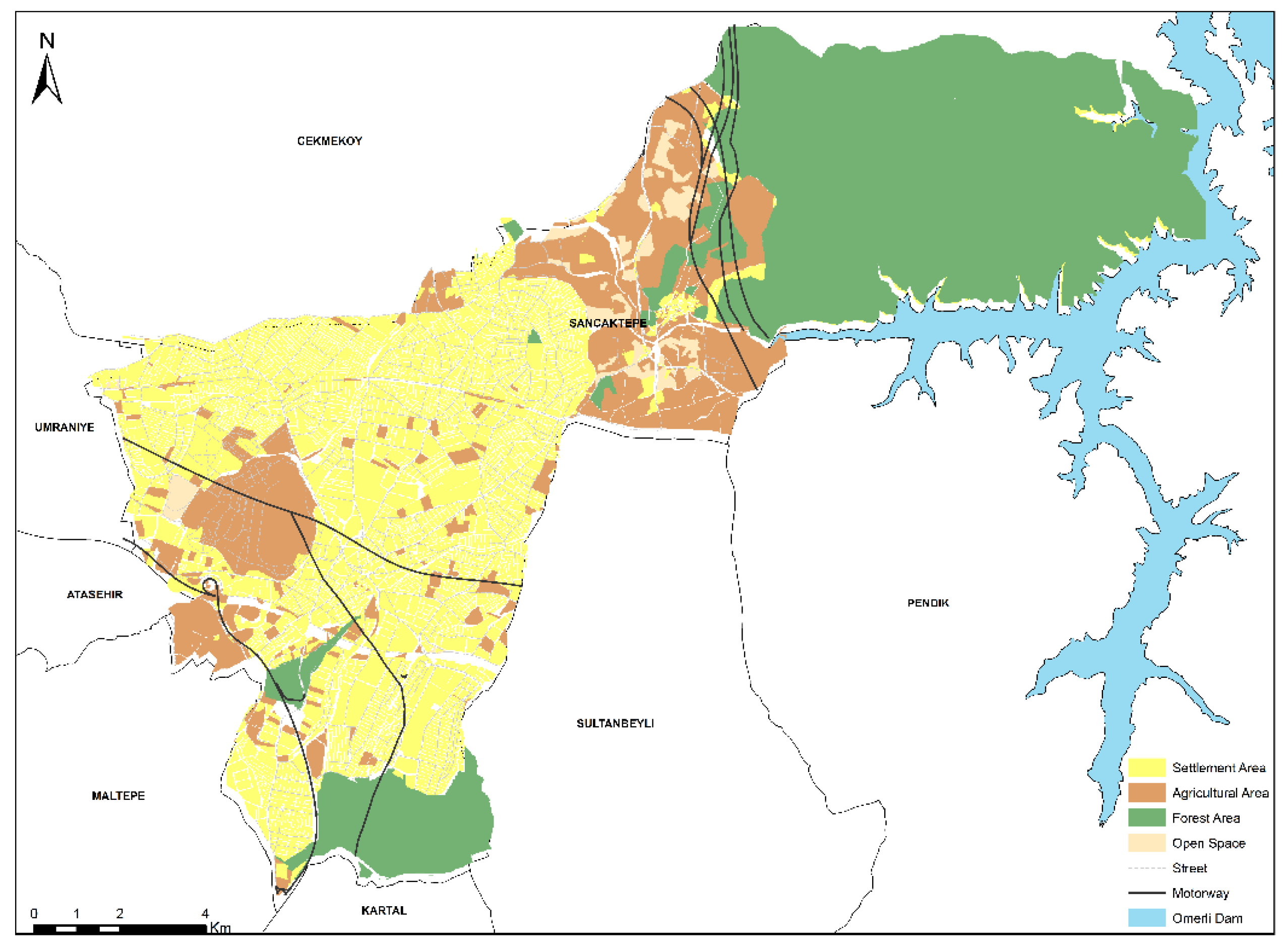
Figure 3.
Land cover for the year 2030 in Sancaktepe.

Figure 4.
Land cover for the year 2050 in Sancaktepe.


Table 1.
Exploratory Factor Analysis (EFA) results for calibration steps.
| Calibration | Kaiser–Meyer–Olkin (KMO) | Bartlett’s Significance (p) | Total Variance Explained (TVE) (%) | Number of Factors | Growth Cycle |
|---|---|---|---|---|---|
| Coarse | 0.50 | 0.000 | 76 | 8 | 3125 |
| Fine | 0.79 | 0.000 | 78 | 2 | 6480 |
| Final | 0.73 | 0.000 | 86 | 2 | 215 |
Table 2.
The highest r2 values according to factor 1 class.
| Product | Compare | Pop | Edges | Clusters | Cluster Size | Lee-Salee | Slope | % Urban | X-mean | Y-mean | Rad | F-match | |
|---|---|---|---|---|---|---|---|---|---|---|---|---|---|
| Coarse | 0.01347 | 0.35701 | 0.98925 | 0.76009 | 0.52615 | 0.99984 | 0.15345 | 0.96154 | 1.00000 | 0.99674 | 0.88642 | 0.99754 | 0.73343 |
| 0.01706 | 0.35863 | 0.99426 | 0.91684 | 0.56293 | 0.99986 | 0.15177 | 0.95750 | 0.99975 | 1.00000 | 0.87183 | 0.99947 | 0.73247 | |
| 0.01064 | 0.35558 | 0.99618 | 0.99614 | 0.57660 | 0.97643 | 0.15373 | 0.89470 | 0.99506 | 0.85782 | 0.62254 | 1.00000 | 0.73256 | |
| Fine | 0.00158 | 0.36305 | 0.99669 | 0.05183 | 0.92907 | 0.99979 | 0.15149 | 0.93948 | 0.99950 | 0.99615 | 0.87798 | 0.99994 | 0.73063 |
| 0.00074 | 0.36303 | 0.99661 | 0.02489 | 0.92257 | 0.99993 | 0.15127 | 0.94080 | 0.99950 | 0.99945 | 0.85189 | 0.99993 | 0.73093 | |
| 0.00367 | 0.36276 | 0.99723 | 0.12215 | 0.90784 | 0.99962 | 0.15143 | 0.93535 | 0.99934 | 0.96659 | 0.91423 | 0.99999 | 0.73201 | |
| Final | 0.00980 | 0.38958 | 0.98620 | 0.59272 | 0.89999 | 0.97937 | 0.14959 | 0.77175 | 0.98388 | 0.91453 | 0.66347 | 0.97941 | 0.72323 |
Table 3.
Selecting coefficient ranges.
| Coefficient Name | From Coarse | From Fine | From Final | From Forecast | ||||||
|---|---|---|---|---|---|---|---|---|---|---|
| Start | Step | Stop | Start | Step | Stop | Start | Step | Stop | Best Fit Values | |
| Diffusion | 50 | 5 | 75 | 75 | 1 | 75 | 75 | 1 | 75 | 66 |
| Breed | 75 | 5 | 100 | 95 | 1 | 100 | 96 | 1 | 96 | 66 |
| Spread | 50 | 5 | 75 | 75 | 1 | 75 | 75 | 1 | 75 | 66 |
| Slope | 0 | 25 | 100 | 95 | 1 | 100 | 95 | 1 | 95 | 49 |
| Road gravity | 0 | 5 | 25 | 0 | 5 | 25 | 25 | 1 | 25 | 40 |
© 2019 by the author. Licensee MDPI, Basel, Switzerland. This article is an open access article distributed under the terms and conditions of the Creative Commons Attribution (CC BY) license (http://creativecommons.org/licenses/by/4.0/).
Share and Cite
MDPI and ACS Style
Ayazli, I.E. Monitoring of Urban Growth with Improved Model Accuracy by Statistical Methods. Sustainability 2019, 11, 5579. https://doi.org/10.3390/su11205579
AMA Style
Ayazli IE. Monitoring of Urban Growth with Improved Model Accuracy by Statistical Methods. Sustainability. 2019; 11(20):5579. https://doi.org/10.3390/su11205579
Chicago/Turabian StyleAyazli, Ismail Ercument. 2019. "Monitoring of Urban Growth with Improved Model Accuracy by Statistical Methods" Sustainability 11, no. 20: 5579. https://doi.org/10.3390/su11205579
Note that from the first issue of 2016, this journal uses article numbers instead of page numbers. See further details here.