Article

Uncertainty of Energy and Economic Performance of Manual Solar Shades in Hot Summer and Cold Winter Regions of China

1
Department of Architecture, Ningbo University, Ningbo 315211, China
2
Department of Civil Engineering, Ningbo University, Ningbo 315211, China
*
Author to whom correspondence should be addressed.
Sustainability 2019, 11(20), 5711; https://doi.org/10.3390/su11205711
Submission received: 19 September 2019 / Revised: 11 October 2019 / Accepted: 14 October 2019 / Published: 16 October 2019
(This article belongs to the Special Issue Building Energy Assessment)

Abstract

:
Occupant behavior is recognized as a major source of discrepancy between simulated and actual energy consumption. This study investigates the uncertainty of energy and economic performance of manual solar shades for the south facade. A developed stochastic model for manual solar shades based on a discrete-time Markov chain method was constructed in Building Controls Virtual Test Bed (BCVTB) for co-simulation with EnergyPlus. The stochastic shade model was compared with deterministic models concerning energy savings potential and life cycle economic performance at different building scales (i.e., from a single room to a whole building). The results show that annual energy uncertainty, due to occupant behavior, on manual shades can be neglected at the building level, whereas for sizing heating equipment, energy uncertainty should be considered. The payback period for manual shades is about 10 years and, in general, a larger building has a higher economic performance. Comparative analysis shows that there is a relatively big performance overestimation or underestimation by commonly used deterministic models in building simulation tools, and thus may lead to a biased economic analysis or even an inappropriate design decision when comparing different energy-saving measures.

1. Introduction

1.1. Importance of Solar Shading Devices

Solar shading devices represent one of the most important bioclimatic components and are popular strategies used by designers to improve façade performance. The use of solar shading systems presents a crucial aspect in improving energy efficiency in buildings. Many design standards and codes for building energy efficiency require an application of solar shading systems for reducing solar heat gain in summer. Among different types of shading, movable solar shading devices play a critical role in balancing various aspects of indoor environmental quality, such as daylight levels, discomfort glare, view to outside, privacy, and thermal comfort. Thus, they are widely used in buildings either manually operated or motorized controlled by the building automation system. Due to low initial and maintenance costs, manual solar shades are widely used instead of automated ones in glazed office buildings in hot summer and cold winter zones of China [1].
Manual shades highly rely on occupants’ control, and thus the performance of manual shades has a great uncertainty since occupant behavior is stochastic rather than deterministic [2].Previous research has shown that occupant behavior significantly influences building energy use and it is considered to be one of the most important factors of building performance simulation [2,3]. Therefore, the prediction of energy performance of manual shades should take into account behavior characteristics, to have a better estimate of the energy savings and economic performance of manual shades (such as life cycle payback periods of manual shades).

1.2. Literature Review

To simulate the energy uncertainty of manual shades, shade behavior models need to be developed. Recently, a few studies have been conducted in this area. For example, Mahdavi et al. [4] investigated occupants’ operation of lighting and shading systems in office buildings. They found that a linear relationship can be used to describe the correlation between shade closing behavior and solar radiation, however, the proposed regression model only produces deterministic shade positions at a certain condition (stochastic shade positions cannot be simulated). According to several comprehensive reviews, most of the existing window blind and shade use models are deterministic [5,6,7] rather than stochastic. For example, manual shades were only triggered by environmental parameters in a few research studies, such as workplane illuminance [8], daylight glare [9], and solar radiation [10], without considering occupants’ impact. Reinhart [11] developed a model for manual control of electric lighting and blinds. The main limitations of this model are that (1) it is based on a rigid solar threshold (thus not stochastic) and (2) only two shade positions are considered (fully opened or fully closed), which is not in line with the real situation that windows may be partially shaded by blinds.
To introduce a certain level of stochastic characteristic, a comprehensive blind use model that considers partial shading events was developed by Haldi and Robinson [12] based on logistic regression curves, however, it was based on a rather unusual external blind configuration (included two motorized blinds with one lower blind covering the totality of the vision window and an upper blind covering an anidolic system), leading to shade positions being mostly fully open and fully closed (around 75% of occupied periods) which is not in line with the real situation in other buildings (partly shading positions) [13]. According to Da Silva et.al. [14], it is important to consider intermediate positions in building performance simulation rather than only extreme ones (either fully deployed or fully retracted). Thus, the generalization of this blind model is limited to this particular building. A literature review of these shade models and their limitations is described in Table 1.
Due to the uncertainty of occupant behavior, actual building energy performance is also uncertain, and thus building performance should be expressed as a probability distribution rather than a single deterministic value [15]. A few studies have reported the uncertainty of energy performance related to occupant behavior (see Table 2). For example, Clevenger and Haymaker [16] simulated the impact of occupants’ behavior on building energy demand by considering high and low energy use behaviors. The results showed that energy consumption might change by more than 150% when occupants with different energy characteristics are considered. Similar studies on lighting energy uncertainty using light switch models [17,18] and on cooling or heating energy uncertainty using different energy use patterns have also been reported.
Due to limited availability of shade behavior models, the uncertainty of energy performance related to manual shades has rarely been studied by researchers. Only a few researchers reported energy uncertainty related to manual shades. For example, Sara et al. [20] simulated occupants’ impact on lighting performance at different spatial scales. They compared Haldi’s shade model with other schedule and rule-based shade models, however, this research did not consider cooling and heating energy uncertainty. A few researchers [21,22] simulated building energy performance by considering different occupant behaviors (such as window opening, shade adjustment, and occupancy), however, the energy uncertainty resulting from manual shades alone cannot be directly obtained from these studies since they only gave the overall impact of different occupant behaviors. Additionally, they all used Haldi’s shade model, which is an unusual shade configuration, as mentioned above. Meanwhile, Haldi’s model is developed based on motorized shading systems, which leads to a high percentage (over 70%) of fully open or closed shade positions. This is because shades of that building are set in motion by pressing one command while another press is needed for stopping it, whereas for manual shades used in China, there is a big difference in shade handling easiness as compared to shades in Haldi’s research. Most of the manual shades in China require users to pull the control chain to either lower or raise the shade to the desired height, and thus shade positions are mostly intermediate ones (partly shading) [1], which means Haldi’s shade model is very building specific and possibly not suitable for other buildings [14].

1.3. Research Gaps

Due to limitations of existing shade behavior models described above, energy and uncertainty prediction of manual shades may be biased. In addition to energy performance, life cycle economic performance of manual shades by considering occupant behavior uncertainty is also an important factor in comparing different design solutions. However, this aspect, to the best of authors’ knowledge, has not been studied since most shade models are deterministic (not suitable for uncertainty analysis of economic performance). Thus, there is a need to investigate the energy uncertainty of manual shades and its economic performance by considering the uncertainty of occupant behavior. A more general shade behavior model, based on widely used manual shades in China, was developed by [1] using the Markov Chain method and this model has been coupled with simulation tools for predicting energy performance of manual shades. This study uses this shade behavior model to conduct simulation studies on the energy and economic performance of manual shades and gives performance comparison with currently used deterministic shade models.

2. Methodology

2.1. Office Cell

A typical office cell was considered in this study. Its dimensions are 4 × 4 × 3 m with a 3.8 × 2.8 m window on the south façade, as shown in Figure 1 (other facades are not considered in this research but can be studied similarly). The characteristics of the office cell (including the setting of manually controlled external shading devices), as well as energy simulation settings, are shown in Table 3. The stochastic shade model used in this study is described in the following section.

2.2. The Stochastic Model of Manual Solar Shades

To investigate the uncertainty of energy and economic performance of manual solar shades, the stochastic shade model developed in a previous study by [1] was used in this study. This model was constructed based on field measurements (monitored shade positions and outdoor weather conditions) on a high-rise glazing building, in China. Ten office rooms of the south facade were monitored, and shade behavior of these rooms were used to develop a shade behavior model. In this model, the occupants’ stochastic behavior of solar control was divided into five discrete solar shading states (shaded window ratio of 1, 0.75, 0.5, 0.25, and 0). In this study, shading coefficient (SC) is used to represent these five shading states and its corresponding values are 0, 0.25, 0.5, 0.75, and 1, respectively, which is calculated by 1 minus shaded window ratio. The stochastic adjustment of solar shades was predicted based on the current shade state and solar intensity on the facade using the first order and discrete-time Markov Chain method. The stochastic model for solar shades was modeled in Building Controls Virtual Test Bed (BCVTB) for co-simulation with Energy Plus, an energy simulation engine developed by Lawrence Berkeley National Laboratory. A brief description on how this stochastic model is constructed is shown in Figure 2. More detailed information of this stochastic model and the co-simulation can be found in the previous study [1].

2.3. Uncertainty Index

2.3.1. Shade Control Behavior

To account for the uncertainty of occupant behavior, the shade behavior model used in this study is based on the Markov Chain method, which is a random process. Thus, shade adjustment generated by the behavior model is random and the resulting SC sequences (there is a total of 8760 SC values for an hourly energy simulation) generated for repeated simulation runs are different. An index used to assess how uncertain between two variables (here, hourly SC values between different simulations) is the correlation coefficient. A value of +1 indicates a perfect positive correlation, −1 represents a totally negative correlation, and 0 corresponds to an absence of linear correlation. Because SC values in this study are discrete and ordinal, Spearman rank correlation, a nonparametric test, is used. The Spearman rank correlation test does not carry any assumptions about the distribution of the data, and thus is appropriate for correlation analysis for SC values.

2.3.2. Energy Performance

For uncertainty of energy performance, the probability density function (PDF) was used to fit the data. In this study, normal distribution was adopted (since the following analysis in Section 3.2 confirmed the normal distribution of the data) which uses a two-parameter family of curves. The first parameter, μ , is the mean, the second, σ , is the standard deviation, and the normal PDF of the energy data ( f ( x ) ) can be expressed as [23]:
f ( x ) = 1 σ 2 π exp ( ( x μ ) 2 2 σ 2 )
Using the above fitting analysis, the distribution of predicted energy demand (cooling, heating, and total, in this study) can be determined and then the Monte Carlo analysis can be conducted by sampling from these normal distributions to determine energy uncertainty, which can be calculated as follows using the coefficient of variation index [20]:
C V = σ μ × 100 %
Energy uncertainty for annual heating, cooling, and total were calculated and compared. To understand the impact of building scales on energy uncertainty, different room numbers ranging from 1 to 200 were considered by summation of sampled energy demand (e.g., 50 rooms require 50 samplings and the summation of these 50 sampled energy data was assumed to be the energy demand of these 50 rooms). Since the Monte Carlo analysis is random, a total of 1000 repeated samplings (10 times higher than the suggested number [24]) were conducted for each building scale. In addition, theenergy performance of manual shades as compared to bare windows (clear double-pane window without manual shades) was calculated and the uncertainty of energy savings as compared with bare windows was quantified.

2.4. Number of Repeated Simulations

Because the developed shade behavior model mimics occupants’ random interaction with solar shades, the simulation output (here, it is energy demand) of this behavior model is stochastic. Thus, repeated simulation runs are needed to understand the possible distribution of the simulation output. Therefore, the Monte Carlo analysis was adopted to analyze the uncertainty of energy performance. As described in [22], additional simulation time needed for Monte Carlo can be considered as a weakness. Thus, this study calculates the required minimum number of simulations according to the graphical method recommended in [25]. The minimum number of repeated simulations required is defined by the point at which the line (the cumulative mean of the simulation output) becomes flat (no upward or downward trend).

2.5. Economic Analysis

The uncertainty of energy performance of manual shades directly influences its life cycle economic performance (here, it is denoted as LCE). Therefore, the whole life cycle energy savings during its operation stage should take into account the time value of money and the whole range of costs. The widely used net present value (NPV) in economic analysis was used to calculate the LCE of manual shades. The net present value method is a popular capital budgeting technique that takes into account the time value of money. It can be calculated as [26]:
L C E = N P V = t = 1 N E t · P · ( 1 + i ) t ( 1 + d ) t I
where I is the life cycle cost (here, it is 1596 RMB and 1 USD is about 7 RMB) according to the price of manual shades (the market price of 150 RMB/m2) and its area (10.64 m2)), P is the price of energy (1 RMB per kWh), i is the annual energy inflation rate (here, 0.025 was considered according to its value in the recent 5 years), d is the market discount rate (here, the long-term interest rate of 0.049 in China was considered), t is from 1 to N, and N is the life span of a typical building (here, different years ranging from 1 to 50 were considered since most buildings in China have a life span of only about 30 years). Et is the total energy savings as compared to bare windows at t year(s) which is a random value due to the uncertainty of occupant behavior, and therefore Et is randomly sampled from the fitted distribution (which is further given in Section 3.2) of the Monte Carlo simulation outputs. Due to the randomness of Et, NPV is also a random value, and thus 1000 repeated sampling was conducted to have a better understanding of the probability distribution of NPV.

2.6. Comparison of Behavior Models with Deterministic Models

Current building simulation tools, such as EnergyPlus, have not incorporated probabilistic shade models, and thus manual shade control is mainly modeled as deterministic behavior in simulation tools such as schedule or incident solar radiation-based control [14]. To compare the difference of energy and economic performance between deterministic shade models and the probabilistic model used in this study, two types of deterministic models were considered. The first one is schedule-based control, which assumes that movable shadings are never active during the heating season and that 70% of the glazing area is shaded during the cooling season. The second one is incident solar radiation-based control, which assumes that the shading devices are used whenever the intensity of the solar irradiation on the window exceeds 300 W/m2. These two deterministic models have been widely used in research and standards such as EN ISO 13790 Energy performance of buildings—Calculation of energy use for space heating and cooling [27].

3. Results and Discussion

3.1. Uncertainty of Shade Control

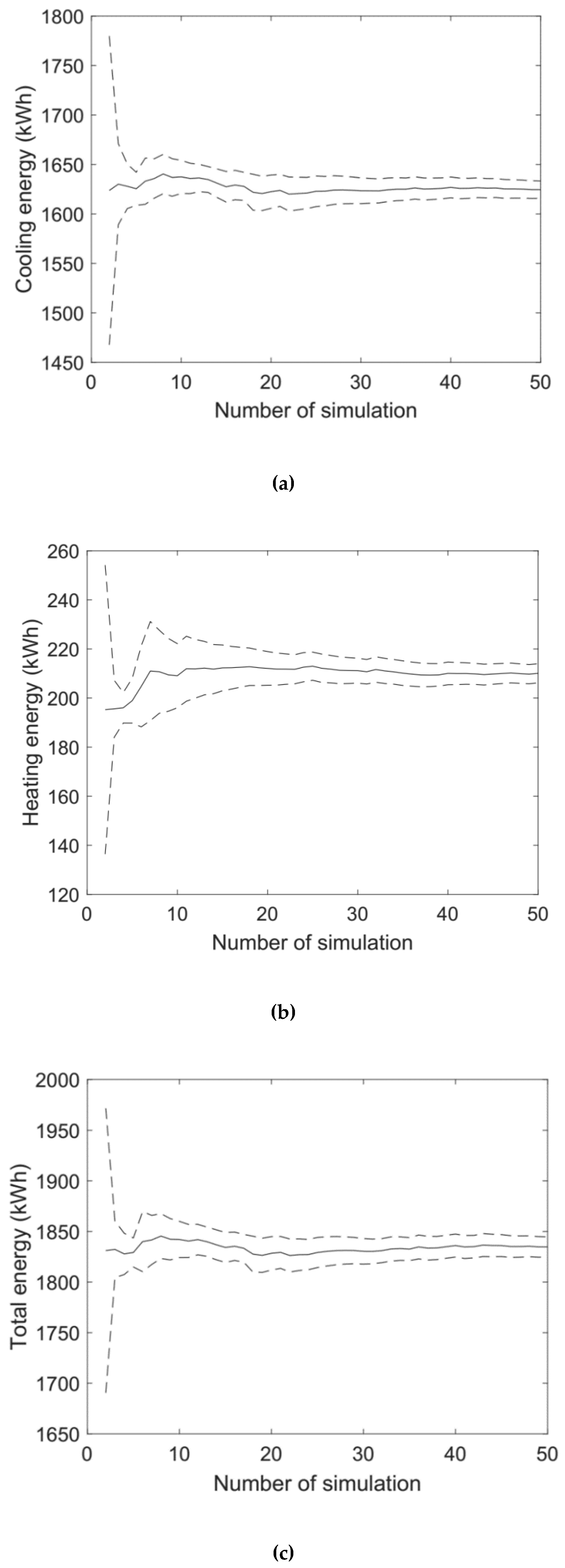
Figure 3 shows hourly SC values of two example simulations during the entire year and shows that the SC values differs largely between the two repeated simulations, although the same shade behavior model is used. Figure 4 further presents the empirical cumulative distribution of the hourly difference of the SC values of these two example simulations. Due to the stochastic characteristics of occupant behavior, more than 70% of the time during the year, the SC value difference is not zero. Therefore, the Monte Carlo analysis of energy performance was conducted and the required minimum number of simulations to achieve a converged solution was determined based on the graphical method, which is shown in Figure 5. It shows that after approximately 25 Monte Carlo simulations, cooling and heating energy performance reach a converged solution. To have a better uncertainty evaluation, 50 Monte Carlo simulations were selected, in this study, for energy uncertainty analysis.
On the basis of 50 Monte Carlo simulations, Figure 6 presents aheat map of the Spearman correlation coefficient of hourly SC values. On the principal diagonal line, the Spearman correlation coefficient is one, because the calculation is based on the same simulation (e.g., simulation one vs. simulation one). For the non-diagonal elements, most correlation coefficients are close to zero with only a few values reaching about 0.2/−0.2, which means no relationship or a very weak relationship between any two simulations, according to the statistics. Therefore, uncertainty of shade behavior was not suppressed by this behavior model, and thus it can be used to conduct uncertainty analysis of energy performance.

3.2. Energy Uncertainty

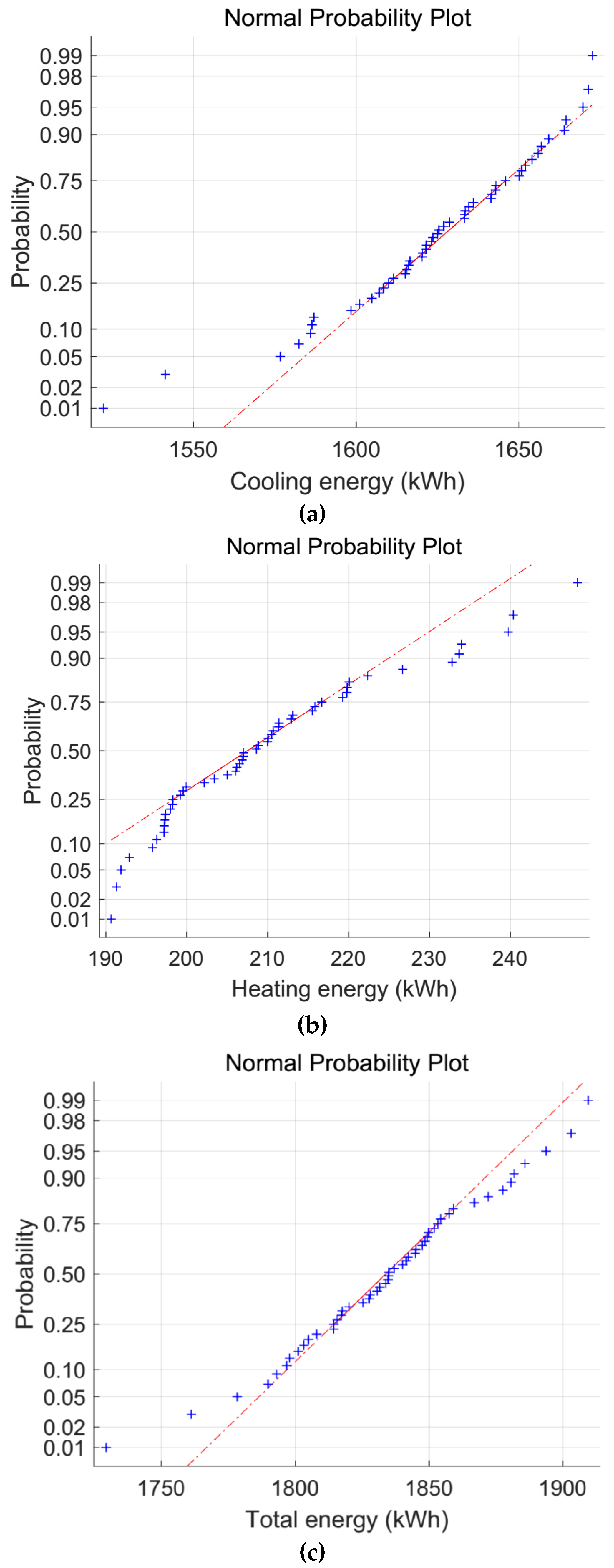
Figure 7 shows the normal probability plot of cooling and heating energy demands (annual heating, cooling, and total energy data for the 50 simulation runs are made available in the public domain as a supplemental file). It shows that energy demands fluctuate significantly among different simulations. For a normal probability plot, if the data points lie approximately on or near the straight line, these data points are likely from a normal distribution. According to Figure 7, cooling, heating, and total energy data seem to follow a normal distribution. Furthermore, a more rigorous statistical test of normality of these energy data was conducted by the Shapiro–Wilk test [28], since the normal probability plot only gives a visual inspection. The test shows that the p-value is 0.2443, 0.0611, and 0.5 for cooling, heating, and total energy, respectively, which is higher than 0.05 (a threshold value), which indicates that the null hypothesis cannot be rejected and the data are normally distributed. Thus, normal fitting was conducted for cooling, heating, and total energy according to Equation (1).
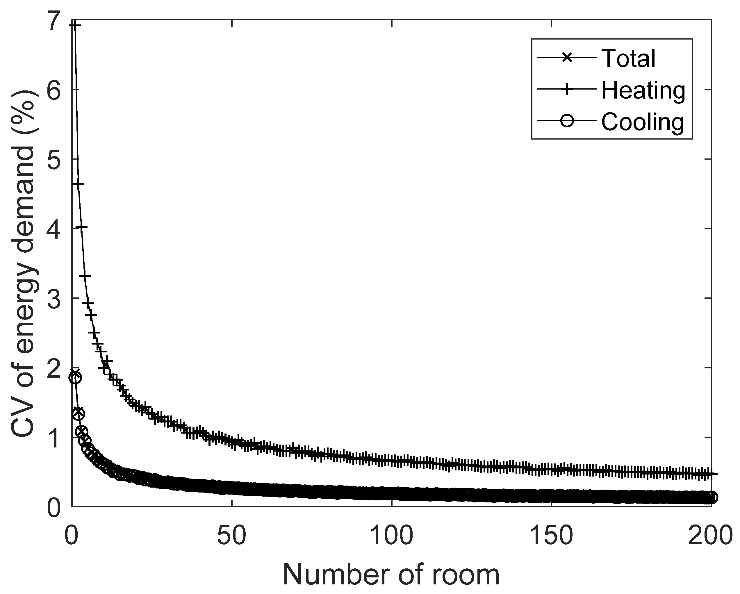
According to the equations described in Section 2.3.2, the uncertainty of cooling, heating, and total energy performance of manual shades were calculated, as shown in Figure 8. It shows that the coefficient of variation (CV) of energy demands of manual shade varies largely with heating, ranging from heating 6.92% to 0.45%. As room numbers increase from one to 200, cooling and total energy demands have very close CV values for different room numbers, ranging from 1.86% to 0.14%. These relative differences (CV)represent the energy uncertainty of manual shades due to stochastic behavior. It can be seen that there is a sharp decrease in the CV to lower than 2% as room numbers increase to higher than 10. This means that the annual energy uncertainty, due to occupant behavior on manual shades, can be neglected for normal office buildings with more than 10 office rooms for one facade, however, it shows that for room-scale, annual heating demand should be given as a probability range rather than a single value due to the large uncertainty. For sizing heating systems of a single room or zone, this uncertainty (>6% for heating) should be considered, whereas for a whole building or cooling system at room level, the uncertainty of occupant behavior on manual shades can be ignored.

3.3. Energy-Saving as Compared to Bare Windows

For bare windows (clear double-pane window without shading), there is no uncertainty for simulated energy performance and its heating, cooling, and total energy is 111.48 kWh, 1916.04 kWh, and 2027.52 kWh, respectively. In comparison to bare windows, there is an increase in heating energy demand due to reduced solar heat transmission into the indoor space in winter by solar shades. The calculated CV values of annual energy savings of manual shades for heating, cooling, and total energy demands (see Figure 9) are higher than the CV of annual energy demands, which is discussed in Section 3.2. The CV of annual heating saving is negative and reduces from 14.21% to 0.95% as the room number increases from one to 200. For cooling and total energy demands, they both perform better than bare windows with fewer energy demands. Due to the relatively high cooling energy savings, the overall impact of manual shades on energy performance is positive. The CV of annual cooling saving is reduced from 10.44% to 0.73%. The combination of these two effects leads to a total energy savings which range from 18.99% to 1.29%. The CV values indicate that there is high uncertainty when evaluating energy savings using manual shades at room level and uncertainty should be taken into consideration for predicting a single room energy performance, whereas for normal office buildings, the uncertainty of energy savings can be ignored.
In a previous study by [29], a comparison of energy savings potential of different energy-saving measures was conducted and found that the total energy savings from a single measure are limited. For example, adding wall insulation materials to reduce wall U values from 1.45 W/m2·K to 0.7 W/m2·K leads to a total energy reduction of only 4.2%, while using Low-E windows instead of clear windows for south façade only achieves an energy reduction of 2.5%. The combination of these two energy-saving measures has an energy savings potential of less than the energy uncertainty (4.2% + 2.5% < 18.99%) due to shade behavior. Thus, this level of total energy uncertainty is significant at room level, however, this influence reduces significantly as the room number increases (i.e., energy uncertainty is less than energy savings resulting from the combination of these two measures) and the choice of energy-saving measures and corresponding economic analysis (such as payback period) regarding manual shades at whole building level does not need to consider the uncertainty of energy savings, which is induced by uncertain occupant behavior.
The shade behavior model used in this study represents typical shade behavior patterns in this climate region. An important behavior feature of manual shades is the duration of keeping a shade unchanged, because occupants lower shades to control direct sun and glare and, then, may forget to adjust the shades for weeks or even months when the source of discomfort is no longer present. This phenomenon can be observed in Figure 10, which shows the boxplot of the duration of keeping a shade unchanged for the first 10 simulation runs. It shows that the maximum duration can reach more than 20 days and the average duration is 58 h. Therefore, this phenomenon (forget to reopen solar shades) has been considered in the energy and the following economic analysis. This also means that the occupants’ shade behavior is sometimes not effective in maximizing daylight utilization.

3.4. Economic Performance

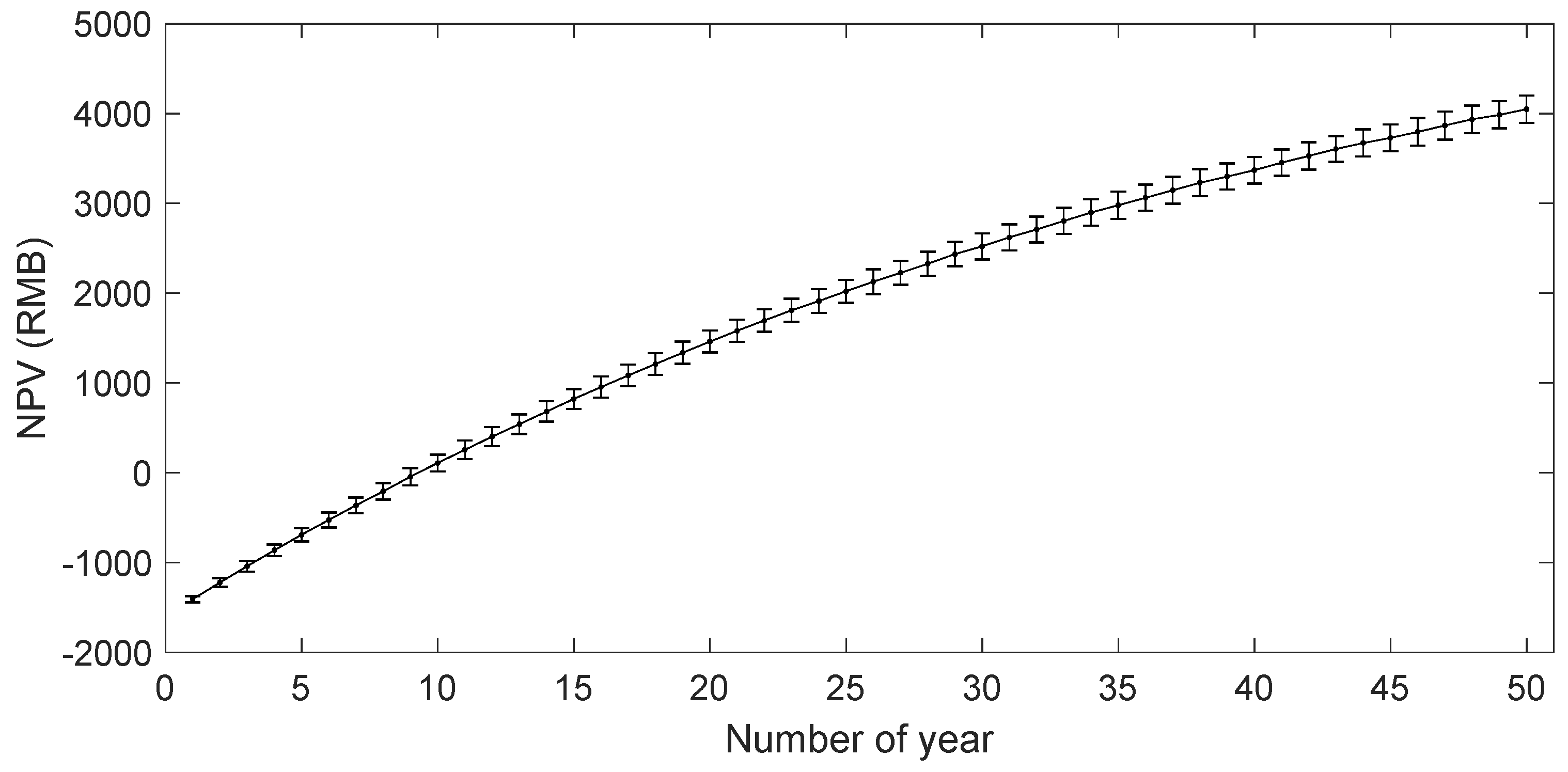
According to the energy performance and the equation described in Section 2.5, the life cycle economic performance (NPV value) of manual shades is illustrated in Figure 11 and shows that the mean NPV increases from about 1500 RMB to 4000 RMB as the number of years increases from one to 50. If the NPV is positive, it means the energy savings is more than the cost and the investment (here, it is the use of manual shades) is acceptable. On the contrary, a negative NPV indicates a net loss and the investment proposal is rejected. It also shows that the LCE of manual shades can be positive or negative, which means decisions of both acceptance and rejection of manual shades can be made depending on the number of years (payback periods) that manual shades have been adopted.
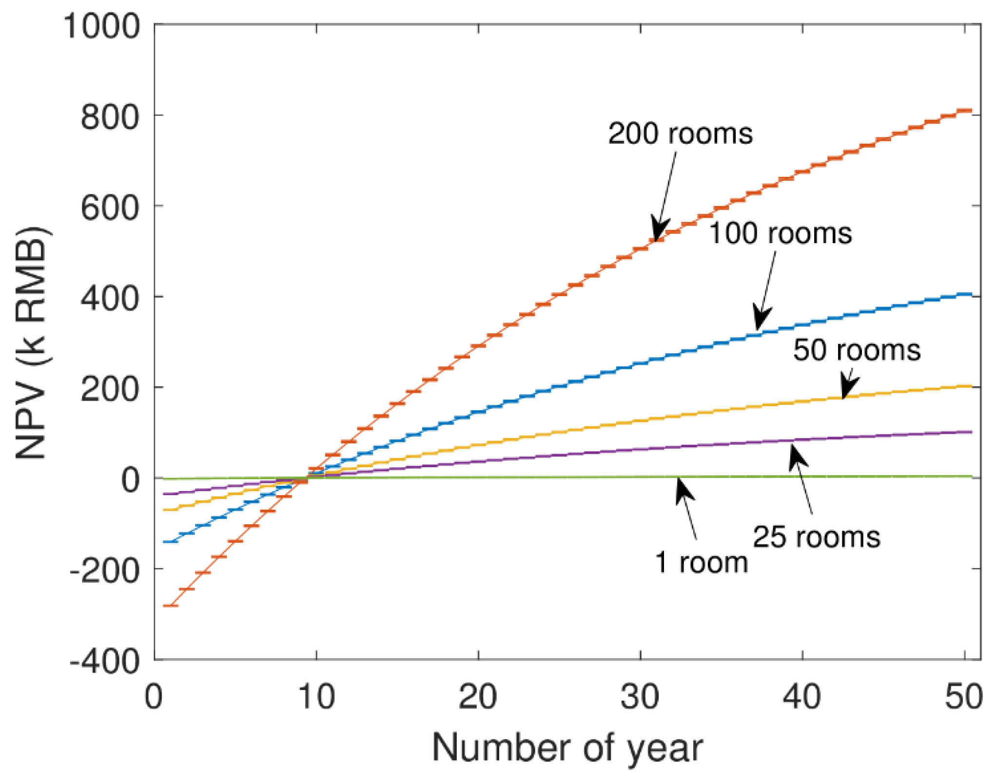
Furthermore, Figure 12 shows the mean NPV and error bar (standard deviation) for different building scales and that the payback period for manual shades is about 10 years (less than life span of normal office buildings). In general, the larger the building is, the higher the NPV it achieves, which means that manual shades are generally economically feasible for office buildings in hot summer and cold winter regions of China. However, if an energy retrofitting of an existing building is going to be conducted by an energy service company using energy management contract(EMC) modes, then, the payback period of manual shades should be taken into consideration.
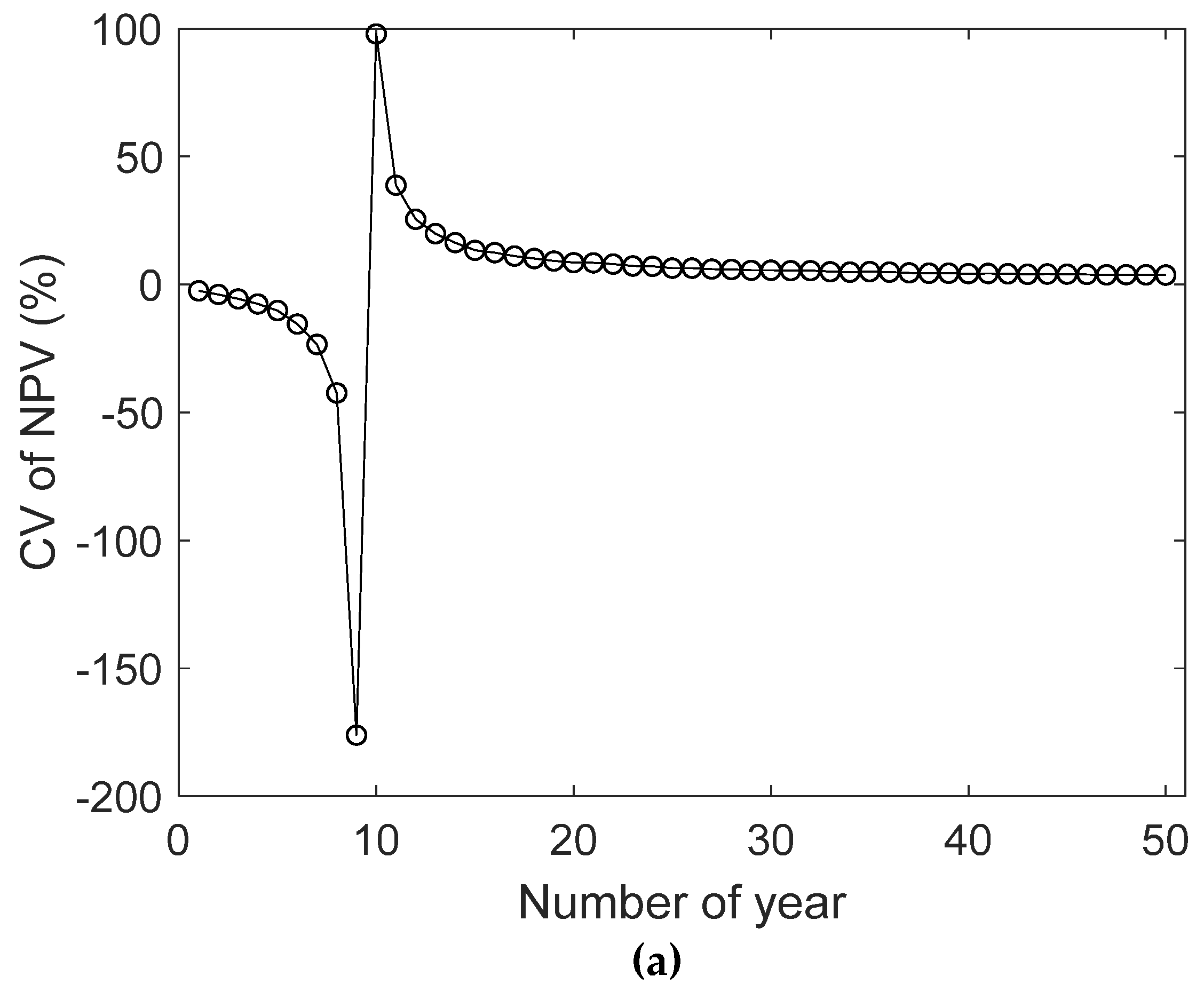
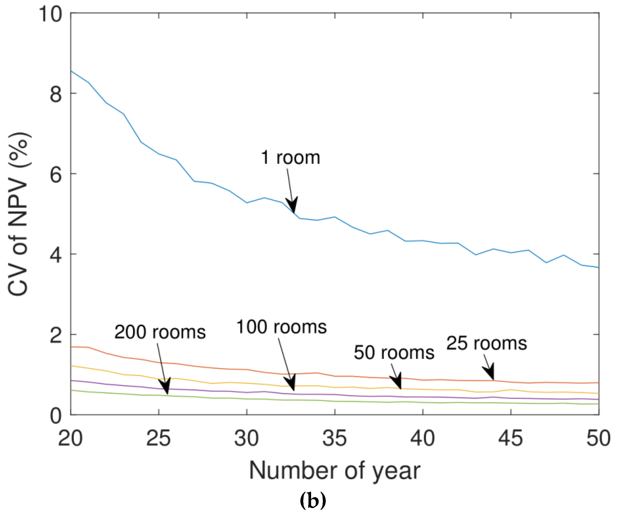
Figure 11 shows that there is the uncertainty of NPV for manual shades, and thus the CV of NPV for different years for the shade behavior model is given in Figure 13. A significant uncertainty of NPV occurs at about 10 years with the CV ranging from 100% to 180% for a single room. This is mainly due to the relatively small mean NPV (approaches zero, the smaller the denominator, the bigger the CV) at around the 10th year. This uncertainty reduces significantly to about 4% as the life span reaches 50 years. Thus, uncertainty of NPV at room level should be considered, whereas for a whole building (different room numbers, see Figure 13b), this uncertainty is much lower (mainly less than 2%) and can be neglected for a typical life span, such as 30 years in China for most buildings.

3.5. Comparison with Deterministic Models

For deterministic shade models, energy simulation results are constant values. The schedule-based model predicts heating, cooling, and total energy demands of 111.48kWh, 1547.04 kWh, and 1658.52 kWh, respectively, whereas for the solar radiation-based model, the predicted heating, cooling, and total energy demands are 253.44 kWh, 1791.88 kWh, and 2045.32 kWh, respectively. The schedule-based shade control predicts a total energy savings of 18.20% as compared with bare windows, whereas for solar radiation-based shade control, its total energy performance is even poorer than bare windows due to increased heating demands (offset cooling reduction), with a total energy increase of 0.88%. The simulation results between deterministic shade models is not only inconsistent, but they are also significantly different from that of the probabilistic shade model (as seen in Table 4). The schedule-based shade control significantly overestimates energy savings, whereas solar radiation-based underestimates energy savings.
For LCE, a comparison of the NPV for a life span ranging from one to 50 years for a single room is given in Figure 14. The NPV for schedule-based control is approximately more than two times higher than that of the shade behavior model, whereas the solar-based assumption leads to an incorrect decision which indicates manual shades are economically infeasible. In addition, the likely distribution of the NPV for the probabilistic model does not cover the other two deterministic assumptions. For other building scales, similar trends are observed, and thus currently the deterministic models are not able to give reliable performance predictions and cannot be used instead of shade behavior models. Meanwhile, there is a relatively big performance overestimation or underestimation by commonly used deterministic models in building simulation tools, which may lead to a biased economic prediction or even an inappropriate design decision when comparing different energy-saving measures.
It should be noted that occupants’ behavior on solar shades is influenced by many factors such as building types, climate, type of shade control, and facade orientation. Life cycle economic performance is also influenced by many factors including the cost of shades and interest rate, etc. The findings of this study should be cautiously interpreted in other cases such as buildings located in different climate regions or equipped with different types of solar shades.

4. Conclusions

This study gives an uncertainty analysis of the energy and economic performance of manual solar shades. A stochastic model developed in a previous study was used in this study for co-simulation. A stochastic shade model was compared with deterministic models concerning energy savings potential and life cycle economic performance at different building scales (i.e., from a single room to a whole building). Results show that annual energy uncertainty, due to occupant behavior, on manual shades can be neglected at the building level, whereas for sizing heating equipment energy uncertainty at room-scale should be considered. A similar conclusion is found for energy savings when compared to bare windows. The economic analysis shows that the payback period for manual shades is about 10 years (less than the life span of normal office buildings) and, in general, the larger the building is, the higher the NPV it achieves, which means that manual shades are generally economically feasible for office buildings in hot summer and cold winter regions of China. The comparison analysis shows that there is a relatively big performance overestimation or underestimation by commonly used deterministic shade models, and thus this may lead to a biased economic prediction or even an inappropriate design decision when comparing different energy-saving measures.
The findings of this research are based on manual shade behavior for the south facade in hot summer and cold winter regions of China and may not be directly applicable to other climates, however, it was found that occupants’ behavior at relatively small spatial scales (e.g., prediction of energy performance at room level) needs to be considered and economic performance of manual shades should be based on a carefully selected shade model (which is capable of representing shade behavior patterns) rather than current simplified shade rules and schedules, which are conclusions that are more general and can also be applied in other climate regions. It should be noted that, in this study, only shade behavior was considered to be stochastic, and other occupants’ behaviors such as cooling and heating schedules and setpoints were considered to be deterministic. This simplification may lead to an underestimation of energy uncertainty in reality since these behaviors may also be stochastic. Thus, a more accurate prediction of energy uncertainty requires consideration of multiple occupants’ behaviors and their possible interactions. Future research efforts are required to identify simplified shade assumptions that can be used for predicting the energy and economic performance of manual shades instead of a stochastic shade model, as well as the applicability of this model to other climate regions and building characteristics and types.

Supplementary Materials

The following are available online at https://www.mdpi.com/2071-1050/11/20/5711/s1.

Author Contributions

The individual contribution and responsibilities of the authors were as follows: Conceptualization, J.Y.; data curation, J.Y.; formal analysis, J.Y.; methodology, J.Y.; writing—original draft, J.Y.; writing—review and editing, J.Y. and R.Z.

Funding

This work was supported by the Natural Science Foundation of Zhejiang Province under grant no. LY18E080012, the National Natural Science Foundation of China under grant no. 51878358, and the National Key Technology R&D Program of the Ministry of Science and Technology under grant 2013BAJ10B06. The author also would like to thank the K. C. Wong Magna Fund at the Ningbo University.

Conflicts of Interest

The authors declare no conflict of interest.

Nomenclature

LCElife cycle economic performance (RMB)
NPVnet present value (RMB)
Ilife cycle cost (RMB)
Pprice of energy (RMB/kWh)
xenergy data for distribution fitting (kWh)
CVcoefficient of variation
Ettotal energy savings as compared to bare windows at t years (kWh)
iannual energy inflation rate
dmarket discount rate
Nthe life span of a typical building (year)
Greek letters
μmean value
σstandard deviation
Subscripts
tthe t-th year which ranges from 1 to N

References

  1. Yao, J. Determining the energy performance of manually controlled solar shades: A stochastic model based co-simulation analysis. Appl. Energy 2014, 127, 64–80. [Google Scholar] [CrossRef]
  2. Yan, D.; Hong, T.Z.; Dong, B.; Mahdavi, A.; D’Oca, S.; Gaetanie, I.; Feng, X.H. IEA EBC Annex 66: Definition and simulation of occupant behavior in buildings. Eng. Build. 2017, 156, 258–270. [Google Scholar] [CrossRef] [Green Version]
  3. Azar, E.; Menassa, C.C. Agent-based modeling of occupants and their impact on energy use in commercial buildings. J. Comput. Civ. Eng. 2012, 26, 506–518. [Google Scholar] [CrossRef]
  4. Mahdavi, A.; Mohammadi, A.; Kabir, E.; Lambeva, L. Occupants’ operation of lighting and shading systems in office buildings. J. Build. Perform. Simul. 2008, 1, 57–65. [Google Scholar] [CrossRef]
  5. Gunay, H.B.; O’Brien, W.; Beausoleil-Morrison, I. A critical review of observation studies, modeling, and simulation of adaptive occupant behaviors in offices. Build. Environ. 2013, 70, 31–47. [Google Scholar] [CrossRef]
  6. O’Brien, W.; Kapsis, K.; Athienitis, A.K. Manually-operated window shade patterns in office buildings: A critical review. Build. Environ. 2013, 60, 319–338. [Google Scholar] [CrossRef]
  7. Van Den Wymelenberg, K.G. Patterns of occupant interaction with window blinds: A literature review. Eng. Build. 2012, 51, 165–176. [Google Scholar] [CrossRef]
  8. Roche, L.; Dewey, E.; Littlefair, P. Occupant reactions to daylight in offices. Light. Res. Technol. 2000, 32, 119–126. [Google Scholar] [CrossRef]
  9. Lee, E.S.; Selkowitz, S.E. The Design and Evaluation of Integrated Envelope and Lighting Control Strategies for Commercial Buildings. Available online: https://escholarship.org/uc/item/3xf9t5rf#author (accessed on 11 October 2019).
  10. Foster, M.; Oreszczyn, T. Occupant control of passive systems: the use of Venetian blinds. Build. Environ. 2001, 36, 149–155. [Google Scholar] [CrossRef]
  11. Reinhart, C.F. Lightswitch-2002: A model for manual and automated control of electric lighting and blinds. Sol. Eng. 2004, 77, 15–28. [Google Scholar] [CrossRef]
  12. Haldi, F.; Robinson, D. Adaptive actions on shading devices in response to local visual stimuli. J. Build. Perform. Simul. 2010, 3, 135–153. [Google Scholar] [CrossRef]
  13. Da Silva, P.C.; Leal, V.; Andersen, M. Occupants interaction with electric lighting and shading systems in real single-occupied offices: Results from a monitoring campaign. Build. Environ. 2013, 64, 152. [Google Scholar] [CrossRef]
  14. Da Silva, P.C.; Leal, V.; Andersen, M. Occupants’ behaviour in energy simulation tools: Lessons from a field monitoring campaign regarding lighting and shading control. J. Build. Perform. Simul. 2015, 8, 338–358. [Google Scholar] [CrossRef]
  15. O’Brien, W.; Gunay, H.B. Mitigating office performance uncertainty of occupant use of window blinds and lighting using robust design. Build. Simul. 2015, 8, 621–636. [Google Scholar] [CrossRef]
  16. Clevenger, C.M.; Haymaker, J. The impact of the building occupant on energy modeling simulations. Civ. Build. Eng. 2006. Available online: http://citeseerx.ist.psu.edu/viewdoc/download?doi=10.1.1.163.2489&rep=rep1&type=pdf (accessed on 11 October 2019).
  17. Yan, D.; Feng, X.H.; Jin, Y.; Wang, C. The evaluation of stochastic occupant behavior models from an application-oriented perspective: Using the lighting behavior model as a case study. Eng. Build. 2018, 176, 151–162. [Google Scholar] [CrossRef]
  18. Zhu, P.; Gilbride, M.; Yan, D.; Sun, H.S.; Meek, C. Lighting energy consumption in ultra-low energy buildings: Using a simulation and measurement methodology to model occupant behavior and lighting controls. Build. Simul. 2017, 10, 799–810. [Google Scholar] [CrossRef]
  19. Zhou, X.; Yan, D.; Feng, X.H.; Deng, G.W.; Jian, Y.W.; Jiang, Y. Influence of household air-conditioning use modes on the energy performance of residential district cooling systems. Build. Simul. 2016, 9, 429–441. [Google Scholar] [CrossRef]
  20. Gilani, S.; O’Brien, W.; Gunay, H.B. Simulating occupants’ impact on building energy performance at different spatial scales. Build. Environ. 2018, 132, 327–337. [Google Scholar] [CrossRef]
  21. Parys, W.; Saelens, D.; Hens, H. Coupling of dynamic building simulation with stochastic modelling of occupant behaviour in offices-a review-based integrated methodology. J. Build. Perform. Simul. 2011, 4, 339–358. [Google Scholar] [CrossRef]
  22. Chapman, J.; Siebers, P.; Robinson, D. On the multi-agent stochastic simulation of occupants in buildings. J. Build. Perform. Simul. 2018, 11, 604–621. [Google Scholar] [CrossRef]
  23. Yao, J. Modelling and simulating occupant behaviour on air conditioning in residential buildings. Eng. Build. 2018, 175, 1–10. [Google Scholar] [CrossRef]
  24. Macdonald, I.A. Comparison of sampling techniques on the performance of Monte Carlo based sensitivity analysis. In Proceedings of the Eleventh International IBPSA Conference, Glasgow, UK, 27–30 July 2009. [Google Scholar]
  25. Robinson, S. Simulation: The Practice of Model Development and Use; Palgrave Macmillan: London, UK, 2014. [Google Scholar]
  26. Yao, J. A multi-objective (energy, economic and environmental performance) life cycle analysis for better building design. Sustainability 2014, 2, 602–614. [Google Scholar] [CrossRef]
  27. CEN, EN ISO 13790. Energy Performance of Buildings-Calculation of Energy Use for Space Heating and Cooling. E.C.F. Standardization. 2008. Available online: http://www.cres.gr/greenbuilding/PDF/prend/set3/WI_14_TC-draft-ISO13790_2006-07-10.pdf (accessed on 11 October 2019).
  28. Prada, A.; Pernigotto, G.; Baggio, P.; Gasparella, A. Uncertainty propagation of material properties in energy simulation of existing residential buildings: The role of buildings features. Build. Simul. 2018, 11, 449–464. [Google Scholar] [CrossRef]
  29. Yao, J. A new design optimization method for energy and indoor thermal performance of apartment buildings. Eng. Eng. 2018, 115, 23–37. [Google Scholar] [CrossRef]
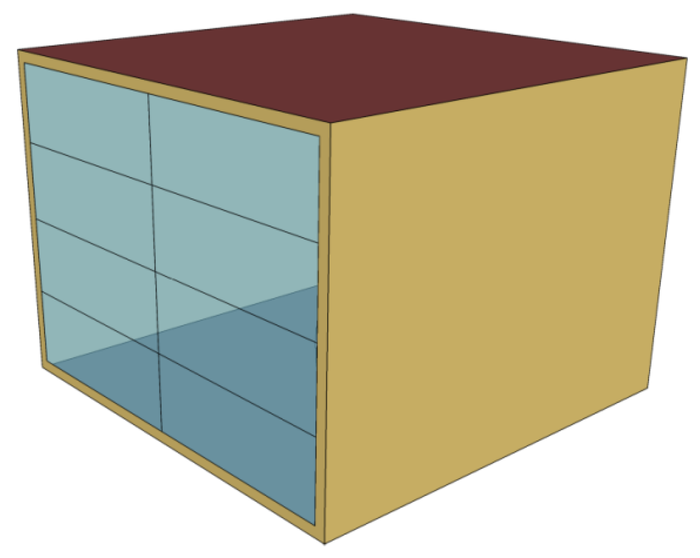
Figure 1. Office cell.
Sustainability 11 05711 g001
Figure 2. A graphic illustration of the developed method for co-simulation of the energy performance of manual solar shades.
Sustainability 11 05711 g002
Figure 3. Hourly SC values of two example simulations during the whole year.
Sustainability 11 05711 g003
Figure 4. Empirical cumulative distribution of hourly difference of SC values of two example simulations during the whole year.
Sustainability 11 05711 g004
Figure 5. The convergence of energy performance, (a) cooling, (b) heating, and (c) total.
Sustainability 11 05711 g005
Figure 6. Heat map of the correlation coefficient of hourly SC values between every two simulations (1,2, …, 50 represent simulation one, simulation two, …, simulation50).
Sustainability 11 05711 g006
Figure 7. Probability plot of cooling and heating energy demands:(a) cooling, (b) heating, and (c) total.
Sustainability 11 05711 g007
Figure 8. The coefficient of variation (CV) of annual energy demand for different building scales for the shade behavior model.
Sustainability 11 05711 g008
Figure 9. Uncertainty of annual energy savings of manual shades for different building scales as compared with bare windows.
Sustainability 11 05711 g009
Figure 10. Box plot of the duration of keeping a shade unchanged for the first 10 simulation runs.
Sustainability 11 05711 g010
Figure 11. Mean net present value (NPV) and error bar (standard deviation) for different years for the shade behavior model.
Sustainability 11 05711 g011
Figure 12. Mean NPV and error bar (standard deviation) for different building scales for the shade behavior model.
Sustainability 11 05711 g012
Figure 13. The CV of NPV for different years for the shade behavior model. (a) The CV of NPV for a single room at a life span ranging from 20 to 50 years and (b) the CV of NPV for different building scales at a life span ranging from 20 to 50 years.
Sustainability 11 05711 g013aSustainability 11 05711 g013b
Figure 14. Comparison of NPV for a life span ranging from 1 to 50 years for a single room.
Sustainability 11 05711 g014
Table 1. Review of manual shade models developed by researchers and their limitations.
YearLiteratureShort Description of Shade ModelLimitations
1995[9]Shades are triggered by daylight glareIt is a deterministic shade model
2000[8]Shades are triggered by workplane illuminanceIt is a deterministic shade model
2001[10]Shades are triggered by solar radiationIt is a deterministic shade model
2004[11]Two types of shade models: dynamic (adjusted daily) and static (permanently lowered)It is based on a rigid solar threshold (thus not stochastic) and only two shade positions are considered (fully opened or fully closed)
2008[4]A linear relationship was developed to describe the correlation between shade closing behavior and solar radiationIt is a deterministic shade model
2010[9]A logistic regression shade model that considers partial shading statesIt is based on a rather unusual external blind configuration
Table 2. Review of occupants’ behavior used for energy uncertainty analysis.
YearLiteratureType of Occupant BehaviorType of Energy Uncertainty
2006, 2012[3,16]Different behavior patterns (e.g., high, medium, and low energy use)Total
2016[19]AC usageCooling
2017, 2018[17,18]Light switchLighting
2018[20]Shade adjustment and light switchLighting
2011, 2018[21,22]Window opening, shade adjustment, light switchCooling and heating
Table 3. Characteristics of the office cell.
ParameterValue
LocationHangzhou city in China, latitude: 30°, longitude: 120°
Orientationsouth
DimensionRoom: 4 × 4 × 3 m, Window: 3.8 × 2.8 m
Window and shading deviceClear double-pane window +manually controlled external shading (Shade, the shade behavior model is described in Section 2.2), shade material: visual transmittance: 0.2.
Work time8:00–17:00
HVACTemperature: 20–26 °C, run time: 8:00–17:00
Interior heat generationLight density: 11 W/m2; equipment: 20 W/m2
Fresh airand 40 m3/h.p
Table 4. Comparison of energy and economic performance between probabilistic and deterministic shade models.
Probabilistic ModelDeterministic Models
Schedule-BasedSolar Radiation-Based
Total energy savings as compared with bare windows (%)9.50(±1.73)18.20−0.88
Note: Negative values of saving indicate an energy increase, not a reduction. For the probabilistic model, it is expressed as mean ± standard deviation.