A Multivariate Modeling Analysis of Commuters’ Non-Work Activity Allocations in Xiaoshan District of Hangzhou, China

Abstract

This paper investigates the outdoor non-work activity allocation behaviors of commuters in Xiaoshan District of Hangzhou, China, as well as the underlying relationship among different types of outdoor non-work activities. As per their commute and work schedules, commuters’ outdoor non-work activities are classified into six categories and considered as binary dependent variables for modeling analysis, including from home before work, on commute way from home to work, going home during work, going out (not going home) during work, on commute way from work back home, and from home after work. Independent variables include commute attributes, work schedules, sociodemographic attributes, and built-environmental attributes. A multivariate probit model is developed to explore the effects of explanatory variables and capture correlations among unobserved influential factors. The model estimation results show that daily work time, education years, and traffic zone have substantial impacts on commuters’ non-work activity allocations. As for the underlying relationship among unobserved factors, a positive correlation is found between the outdoor non-work activities on commute way to and from work, indicating a mutually promotive relationship. All other correlations are negative, indicating other types of non-work activities are mutually substitutive. These findings will help to better understand commuters’ behaviors of outdoor activity arrangement subject to the time-space constraint from fixed work schedules, and shed some light on the mechanism of complex work tour formation, so as to guide the development of activity-based travel demand models for commuters.

1. Introduction

As a developing country with rapid economic development, China has experienced constant population growth and spatial expansion in many large cities. Travel demand keeps growing over time and travel patterns have become increasingly complex. Taking Shanghai as an example, the number of average daily commute trips was 25.11 million in 2014 with an increase of 7% over 2009, while the number of non-work trips reached 27.01 million in 2014 and accounted for 52% of the total number of trips [1]. For the first time, the number of non-work trips exceeded that of work trips in Shanghai.

As known, commute trips are the most important trips for urban residents. With the rise of housing prices in central urban areas and the separation between workplaces and residences, the average commute trip distance of urban residents has become longer than before [1]. People may undertake some non-work activities (such as picking up children and spouses, shopping, etc.) during a commute trip to make an efficient use of time [2,3,4,5,6], which results in the increase of stops in trip chains. In this case, the departure time and mode choice of commuters can be significantly affected by the complexity of the activity-travel pattern, which may change the midway destinations or routes of commute trips. That is to say, the greater frequencies of non-work trips may have great impacts on commuters’ travel patterns and increase road traffic demand during peak hours [7]. With the rapid growth of automobile ownership in china, such phenomena may become increasingly prevalent due to the flexibility and convenience of automobiles. In view of this, it is necessary to investigate how commuters allocate outdoor non-work activities or non-work trips (both can be used interchangeably in this paper), subject to their fixed commute and work schedules. The outdoor non-work activities of commuters have recently received increased attention [8,9,10,11,12,13]. Previous studies have addressed many aspects of non-work trips, such as frequency [7,14], travel time [15,16], departure time choice [17,18], and mode choice [15,19,20]. It is worth mentioning that mode choice of commuters in a multi-stop tour has become an important module. It is easy to understand that automobiles will encourage people to undertake more complex tours because of flexibility and convenience. On the contrary, public transit, with uncertain waiting time and fixed routes, has a limitation to undertake multiple activities in a tour [21,22]. Therefore, the complex trip chains may increase the dependence of travelers on automobiles, which leads to the problems related to auto route choice and optimization, as well as transportation safety [23,24,25,26,27,28,29,30,31]. In order to verify this conclusion, this paper also takes the mode choice of commuters as one of the independent variables.

Reviewing the existing literature, it can be found that there are three shortages in studies on commuters’ non-work trips. First, previous studies mostly focused on one aspect of non-work activities (such as frequency, travel time, etc.) [20,32] and paid little attention to the allocation of commuters for non-work trips with consideration of their fixed work schedules. Secondly, most existing studies only focus on the influencing factors of non-work activities [33] and rarely discussed the internal relationships among non-work activities. Thirdly, most existing studies do not differentiate commuters’ non-work trips as per their work schedules [15,17]. Wu and Ye [7] only focused on two types of outdoor non-work activities based on commuters’ commute schedules, on the way from home to work and from work back home, but did not take account of non-work activities before, during, and after their work schedules. In this paper, commuters’ non-work activities are comprehensively classified into six types according to both their commute and work schedules. In addition, it was shown that there was a promotive relationship between these two types of outdoor non-work activities in Wu and Ye’s research [7].

In order to fill the gaps mentioned above and inspired by Wu and Ye’s earlier research [7], we raise a further question, as follows: Is the promotive relationship universal among different types of outdoor non-work activities? If commuters shop or eat on the way from work back home, they may not go out for shopping or eating again after getting home, which may result in a substitutive relationship between these two types of outdoor non-work activities. Based on this conjecture, in this paper, the outdoor non-work activities of commuters are divided into six categories according to their work schedules, as follows: From home before work, on commute way from home to work, going home during work, going out (not going home) during work, on commute way from work back home, and from home after work (represented by Act1–Act6), which mostly cover all kinds of the daily activities of commuters, except commute and work. The modeling framework of this study is shown in Figure 1. As shown in Figure 1, Act1–Act6 are dependent variables, that is, the commuters’ choice of six types of non-work activities. Values e1–e6 are error terms with mutual influence. Independent variables involve household attributes (e.g., household income, real estate type or price, home location characteristics), individual attributes (e.g., gender, education level), and work attributes (e.g., daily total work time, work staring time and ending time, commute mode, commute distance or time) to explain commuters’ activity or travel behaviours. This framework has been widely accepted in the area of travel behaviour research.

In this paper, a multivariate probit model based on the composite marginal likelihood (CML) estimation approach is applied to quantify impacts from influential factors on the allocation of commuters’ outdoor non-work activities. The error correlations of the multivariate probit model are specified to identify relationships among unobserved factors affecting all types of non-work activity allocations. A positive correlation indicates that two types of outdoor non-work activities are mutually promotive and they are mutually substitutive otherwise. The data are collected from the residents’ household travel survey in Xiaoshan District, Hangzhou, Zhejiang Province in 2015. Xiaoshan District, known as the transportation hub of Zhejiang Province, is one of typical regions of China with a fast-growing economy. This study is helpful for better understanding the commuters’ outdoor activity arrangement behaviors subject to fixed working schedules in order to formulate transportation policies to reduce traffic congestion and vehicle exhaust emissions, and eventually promote the sustainable development in Xiaoshan District.

The rest of this paper is structured as follows. The next section introduces the multivariate probit model and the CML estimation approach. Section 3 presents the descriptive statistics of the sample data and key explanatory variables involved in the model. The estimation results of the model are analyzed in Section 4. The final section summarizes the results of this paper and provides some suggestions for the formulation of transportation policy in Xiaoshan District.

2. Modeling Methodology

In this study, there are six types of outdoor non-work activities for commuters to choose from, including from home before work, on commute way from home to work, going home during work, going out (not going home) during work, on commute way from work back home, and from home after work. For each commuter, there is a binary choice for whether each type of outdoor non-work activity is allocated or not. Thus, the multivariate probit model should be appropriate to model the commuters’ allocations of six types of outdoor non-work activities. The multivariate probit model is described as follows:

$$y_{im}{}^{*}={\mathsf{\beta }}_m^{\prime }{x}_{im}+{\mathsf{\epsilon }}_{im},m=1,\dots ,M,$$

(1)

where $i$ is an index for commuters ($i=1,2,\dots ,I$, where I represents the total number of commuters in the data set) and $m$ is an index ($m=1,2,\dots ,M$) for a binary-response variable. $M=6$ in this paper, while $m$ denotes 6 types of outdoor non-work activities in sequence. The value $y_{im}{}^{*}$ is the utility of commuter $i$ for a type of outdoor non-work activity represented by $m$. The value $y_{im}$ is a binary variable, ($y_{im}\in \left\{0,1\right\}$), reflecting whether commuter $i$ chooses outdoor non-work activities represented by $m$. If $y_{im}{}^{*}$ is greater than 0, it means $m$ is chosen by commuter $i$ and $y_{im}=1$, otherwise $y_{im}=0$. Hence Equation (1) can be rewritten to Equation (2) as follows:

$$y_{im}{}^{*}={\mathsf{\beta }}_m^{\prime }{x}_{im}+{\mathsf{\epsilon }}_{im},m=1,\dots ,M$$

$$y_{im}=\left\{\begin{array}{l}1,y_{im}{}^{*}>0\\ 0,y_{im}{}^{*}\le 0\end{array}\right\},$$

(2)

where $x_{im}$ is a vector of explanatory variables and ${\mathsf{\beta }}_m$ is a corresponding vector of coefficients to be estimated. The value ${\mathsf{\epsilon }}_{im}$ is a stochastic disturbance term, which is used to represent the sum of all influential factors excluded from vector $x$. In this study, the correlations in the ${\mathsf{\epsilon }}_{im}$ terms across variables, $m$, are used to determine whether two kinds of outdoor non-work activities are mutually promotive or substitutive. The value ${\mathsf{\epsilon }}_{im}$ is assumed to be normally distributed. Then, ${\mathsf{\epsilon }}_i={\left({\mathsf{\epsilon }}_{i1},{\mathsf{\epsilon }}_{i2},\dots ,{\mathsf{\epsilon }}_{iM}\right)}^{\prime }$ is multivariate normally distributed with a mean vector of zeros, and a correlation matrix as follows:

$${\mathsf{\epsilon }}_i\sim N\left[0,\mathsf{\Sigma }\right],\mathsf{\Sigma }=\left(\begin{array}{llll}1& {\mathsf{\rho }}_{12}& \cdots & {\mathsf{\rho }}_{1M}\\ {\mathsf{\rho }}_{12}& 1& \cdots & {\mathsf{\rho }}_{2M}\\ ⋮& ⋮& \ddots & ⋮\\ {\mathsf{\rho }}_{1M}& {\mathsf{\rho }}_{2M}& \cdots & 1\end{array}\right).$$

(3)

The off-diagonal terms in correlation matrix $\mathsf{\Sigma }$ indicates the error covariances across underlying continuous random variables, which can capture the effects of unobserved factors influencing utilities. The values on the diagonal terms of $\mathsf{\Sigma }$ are normalized to 1. If all the elements on the off-diagonal equal to 0, then the model in Equation (1) collapses to multiple simple probit models. All error covariances are stacked into a vertical vector $\mathsf{\Omega }$. $Y_i={\left(Y_{i1},Y_{i2},\dots ,Y_{iM}\right)}^{\prime } \left(1\le i\le I\right)$ denotes the choice of commuter $i$ for 6 types of outdoor non-work activities, then the estimated parameter vector of the multivariate probit model is $\mathsf{\delta }={\left({\mathsf{\beta }}_1{}^{\prime },{\mathsf{\beta }}_2{}^{\prime },\dots ,{\mathsf{\beta }}_M{}^{\prime },{\mathsf{\Omega }}^{\prime }\right)}^{\prime }$. The likelihood function of commuter $i$ is given as follows [34]:

$$L\left(\mathsf{\delta }\right)=P_r\left(Y_i=y_i\right)={\displaystyle {\int }_{A_{iM}}{\displaystyle {\int }_{A_{iM-1}}\cdots {\displaystyle {\int }_{A_{i1}}{\mathsf{\phi }}_M\left(\mathrm{z}|0,\mathsf{\Sigma }\right)}}}dz,$$

(4)

where ${\mathsf{\phi }}_M$ is the probability density function of the $M$-variate normal distribution with a mean vector of zeros and a covariance matrix, $\mathsf{\Sigma }$. The above likelihood function is a multi-integral of M-dimension for each commuter $i$ in order to obtain the estimation of parameter $\mathsf{\delta }$ using the maximum likelihood estimation method. The values of $A_{im}$ are as follows:

$$A_{im}=\left\{\begin{array}{l}\left(-\infty ,{\mathsf{\beta }}_m^{\prime }{x}_{im}\right) if y_{im}=1,\\ \left[{\mathsf{\beta }}_m^{\prime }{x}_{im},\left.\infty \right) if y_{im}=0\right.\end{array}\right..$$

(5)

After the model is determined, parameter estimation is of great importance to obtain consistent coefficients and error correlations. It can be found from Equation (4) that the complexity of the model will raise rapidly with the increase of dimension. The estimation of the likelihood function will be extremely difficult without additional restrictions on the covariance matrix. Therefore, the initial application of the multivariate probit model is often limited to two dimensions or three dimensions and cannot be extended to higher dimensions. At present, the methods used to estimate the multivariate probit model are maximum simulated likelihood (MSL) [35], the GHK (Geweke–Hajivassiliou–Keane) simulation method [36,37,38], and the Monte Carlo EM method [34]. In this paper, we use the composite marginal likelihood (CML) estimation method to estimate the multivariate probit model, because the CML method can provide the consistent estimators for both coefficients of explanatory variables and correlations in the error covariance matrix. When the full information maximum likelihood estimation procedure is overly computationally intensive, the composite maximum likelihood method can be an alternative [39,40]. Bhat [41] has demonstrated that the CML method has advantages in computational convenience and stability in spite of some efficiency loss. The pairwise marginal likelihood function for commuter $i$ can be written for the multivariate probit model as follows, whose details are described in the methodological Appendix.

$$L_{CML,i}^{MP}\left(\mathsf{\delta }\right)={\displaystyle {\prod }_{j=1}^{M-1}{\displaystyle {\prod }_{k=j+1}^M\mathrm{Pr}\left(y_{ij},y_{ik}\right)}},$$

(6)

$$={\displaystyle {\prod }_{j=1}^{M-1}{\displaystyle {\prod }_{k=j+1}^M{\mathsf{\Phi }}_2\left({\mathsf{\alpha }}_{ij}{\mathsf{\beta }}_{ij}{x}_{ij,}{\mathsf{\alpha }}_{ik}{\mathsf{\beta }}_{ik}{x}_{ik,}{\mathsf{\alpha }}_{ij}{\mathsf{\alpha }}_{ik}{\mathsf{\rho }}_{j\mathrm{k}}\right)}},where$$

$${\mathsf{\alpha }}_{ij}=2\ast y_{ij}-1, \mathrm{and}$$

$${\mathsf{\alpha }}_{ik}=2\ast y_{ik}-1.$$

3. Data Preparation and Description

3.1. Descriptive Analysis of Sample Data

The data set of this study was collected from the residents’ household travel survey in Xiaoshan District of Hangzhou conducted by Tongji University in 2015. Hangzhou is the capital of Zhejiang Province, and Xiaoshan District is one of the districts of Hangzhou. The district divisions of Hangzhou and Xiaoshan are depicted in Figure 2. Xiaoshan District has a high population density, with an area of 1420 km² (accounting for 8% of Hangzhou’s area) and a population of 1.57 million (accounting for approximately 16% of Hangzhou’s total population). In terms of economic development level, Xiaoshan District has been ranked first in Zhejiang Province for several years. Xiaoshan is also one of the regions with the most developed manufacturing economy in China. Furthermore, the transportation system in Xiaoshan District has been improved, and there are 2 metro lines and 183 bus routes in operation so far. Taking Xiaoshan as a representative study object, this paper will provide a useful reference for other similar areas in China.

The survey was conducted in the form of a home-based questionnaire survey. The sample was drawn from 3500 households (1% of the number of households in the Xiaoshan district), which was randomly selected from 11 zones of Xiaoshan. A 1-day travel diary was completed through face-to-face interviews. The questionnaire is divided into three parts, as follows: Household attributes survey, personal attributes survey, and personal travel survey. The sample includes 16,254 trips reported by 5490 persons from 2566 households. From this sample, 4518 commuters, who at least reported one work trip on the survey day, were further selected for this study.

Table 1. Descriptive analysis of sociodemographic attributes.

Attribute	Percent	Attribute	Percent
Description of household discrete variables
Household size		Home ownership
Mean	4.01	Self-owned house	91.00%
1	0.1%	Rented house	9.0%
2	6.4%	Annual household income [RMB Yuan]1
3	33.0%	≤100,000	30.0%
4	26.3%	100,000–300,000	58.5%
5	23.7%	300,000–500,000	9.9%
6	8.3%	500,000–1000,000	1.4%
7+	2.2%	≥1000,000	0.2%
The population under the age of 6		Zone
Mean	0.31	Beigan Street	14.5%
0	71.3%	Chengxiang Street	24.4%
1	26.1%	Ningwei Town	10.0%
2	2.3%	Puyang Town	0.4%
3+	0.3%	Shushan Street	13.3%
Real estate price (RMB Yuan/m2)		Suoqian Street	2.9%
Mean	9051	Wenyan Street	5.9%
≤10,000	49.5%	ETD Zone2	4.8%
10,000–15,000	46.6%	Xinjie Town	7.3%
15,000–20,000	3.2%	Xintang Street	16.0%
20,000–30,000	0.5%	Yanqian Town	0.4%
>30,000	0.2%
Description of individual discrete variables
Gender		Licensed commuters
Female	45.8%	Have a license	71.5%
Male	54.2%	Not have a license	28.5%
Profession		Education
Blue collar worker	10.2%	Below primary school	0.7%
Clerk	60.5%	Elementary school	4.9%
Private enterprise head	3.3%	Junior high school	13.8%
Business service staff	4.7%	Senior high school	21.3%
Student	0.3%	Technical secondary school	13.2%
Self-employed	13.4%	Junior College	28.8%
Public officer	4.6%	Bachelor	16.7%
Others	3.0%	Postgraduate	0.6%
Attribute		Mean	S.D.
Description of household continuous variables
Annual household income (10 thousand RMB Yuan)		17.52	10.66
Population density3 (10 thousand people/km2)		0.92	1.443
Description of individual continuous variables
Average education years of commuters (years)		12.78	2.999
Commuter household automobile ownership		1.15	0.702
Commuter household motorcycle ownership		0.07	0.268
Commuter household electric bicycle ownership		1.34	0.820
Commuter household human-powered bicycle ownership		0.32	0.574
Average age of commuters		36.58	8.904

¹ RMB Yuan: Unit of RMB, currency in China; 1 Yuan = approx. US$0.1398. ² ETD Zone is the abbreviation of Economic-Technological Development Zone. ³ Population density is measured by the communities in which the household is located.

shows descriptive statistics of the sociodemographic variables. In this sample, 82% of the commuters have 3–5 people in their families and the average household size is 4.01. About a third of commuter households have children under the age of 6, which indicates that the families with pre-school children account for a significant proportion in the sample. The proportion of commuters who own their home is 91%. While more than 96% of the commuters live in houses with prices below 15,000 RMB Yuan/m². A total of 58.5% of the commuters have annual household incomes ranging from 100,000 to 300,000 RMB Yuan. In order to calculate the average annual household income, the discrete variable of household income is converted into a continuous variable based on the Gaussian distribution. The continuous household income is shown in Table 1, while the average value is estimated at 175,200 RMB Yuan.

According to statistics of individual attributes in Table 1, more than half of commuters are male. In terms of professions, 60.5% of commuters are clerks and 13.4% are self-employed. A total of 71.5% of commuters have driving licenses, which account for a significant proportion in the sample. In the description of the individual continuous variables, the average education years of commuters are 12.78 (about high school) after the discrete education level variable was converted to education years. Each commuter household owns 1.15 automobiles on average, which indicates that the motorization level in the study area is relatively high. In addition, each commuter household owns 0.32 human-powered bicycles on average, which is more than that of motorcycles, but far less than that of automobiles and electric bicycles. The average age of commuters is 36.58.

3.2. Descriptive Analysis of Explanatory Variables and Dependent Variables in the Model

According to statistics of explanatory variables in

Table 2. Descriptive analysis of explanatory variables and dependent variables.

Description of Explanatory Variables
Name	Type	Description	Mean	S.D.
Household sociodemographic attributes
Self-owned house	Dummy	1 if the house is self-owned; 0 otherwise.	0.90	0.302
Rented house	Dummy	1 if the house is rented; 0 otherwise.	0.09	0.283
Real estate price(RMB Yuan/m2)	Categorical	The price of commuter's house.	-	-
Household income(10 thousand RMB Yuan)	Continuous	Annual household income converted from discrete variable in household survey data.	17.71	10.775
Population density(10 thousand people/m2)	Continuous	The population density is obtained based on the small zone level (communities) where the commuter is located.	0.92	1.443
Zone: Street/Town	Categorical	The area (11 streets/towns) where the commuter is located in Xiaoshan District.	-	-
Individual sociodemographic attributes
Gender: Male	Dummy	1 if the commuter is Male; 0 otherwise.	0.54	0.498
Profession	Categorical	The Profession of commuter based on personal survey data.	-	-
Education years of commuters (years)	Continuous	Average education years of commuter based on personal survey data.	12.78	2.999
Trip attributes
Commute mode	Categorical	Travel mode used by a commuter to and from work.	-	-
One-way commute time (minutes)	Continuous	The time required for commuter from home to work (not stopping halfway)	22.60	12.691
Daily work time (hours)	Continuous	Working hours of commuter	9.10	1.705
Work schedule: start at 7–8 a.m. and end at 4–5 p.m.	Dummy	1 if the commuter starts working at 7–8 a.m., and ends working at 4–5 p.m.; 0 otherwise.	0.14	0.348
Work schedule: start at 7–8 a.m. and end at 5–6 p.m.	Dummy	1 if the commuter starts working at 7–8 a.m., and ends working at 5–6 p.m.; 0 otherwise.	0.26	0.438
Work schedule: start at 7–8 a.m. and end at 6–8 p.m.	Dummy	1 if the commuter starts working at 7–8 a.m., and ends working at 6–8 p.m.; 0 otherwise.	0.05	0.214
Work schedule: start at 8–9 a.m. and end at 4–5 p.m.	Dummy	1 if the commuter starts working at 7–8 a.m., and ends working at 4–5 p.m.; 0 otherwise.	0.08	0.271
Work schedule: start at 8–9 a.m. and end at 5–6 p.m.	Dummy	1 if the commuter starts working at 8–9 a.m., and ends working at 5–6 p.m.; 0 otherwise.	0.24	0.425
Work schedule: start at 8–9 a.m. and end at 6–8 p.m.	Dummy	1 if the commuter starts working at 8–9 a.m., and ends working at 6–8 p.m.; 0 otherwise.	0.04	0.184
Description of Dependent Variables
Name	Description		Mean	S.D.
Act1	Nonwork Trip from Home Before Work		0.011	0.103
Act2	Nonwork Trip on Commute Way from Home to Work		0.018	0.134
Act3	Going home during work		0.029	0.168
Act4	Going out (not going home) during work		0.092	0.289
Act5	Nonwork Trip on Commute Way from Work Back Home		0.155	0.362
Act6	Nonwork Trip from Home After Work		0.194	0.396

, all the significant explanatory variables in the developed model are divided into three categories, as follows: household sociodemographic attributes, individual sociodemographic attributes and trip attributes. The name, type, description, mean, and standard deviation of explanatory variables are displayed in the table, respectively.

In this paper, six types of outdoor non-work activities are defined as Act1–Act6, which are described in details in Table 2. The means of Act1 and Act2 are less than 0.02, while the means of Act5 and Act6 are both greater than 0.15. Specifically, the average of Act6 is the largest (0.194), which is over 17.6 times that of Act1. In addition, the mean of Act4 is 0.092, which is nearly 3.1 times that of Act3.

3.3. Distribution Analysis of Purposes of Outdoor Non-Work Activities

Table 3. Crosstab for purpose * act.

	The Types of Outdoor Non-Work Activities
	Act1	Act2	Act3	Act4	Act5	Act6	Total
Shopping and dining	70.83%	29.07%	0.00%	92.57%	56.53%	44.20%	54.40%
Leisure and entertainment	6.25%	4.65%	0.00%	1.92%	13.59%	37.73%	19.44%
Visiting relatives and friends	0.00%	4.65%	0.00%	1.20%	10.77%	10.80%	7.98%
Medical treatment or visiting the sick	2.08%	1.16%	0.00%	1.20%	4.71%	1.59%	2.43%
Companying	20.83%	53.49%	0.00%	1.68%	8.48%	3.64%	6.85%
Going home	0.00%	0.00%	100.00%	0.00%	0.00%	0.00%	5.68%
Others	0.00%	6.98%	0.00%	1.44%	5.92%	2.05%	3.21%
Total	100.00% (N = 48)	100.00% (N = 86)	100.00% (N = 131)	100.00% (N = 417)	100.00% (N = 743)	100.00% (N = 880)	100.00% (N = 2305)

provides purpose distribution of six types of outdoor non-work activities. Act3 is not involved in the discussion below, as its purpose is all for going home. Shopping and dining account for the largest proportion in all the types of outdoor non-work activities, except Act2. Especially, the proportion of shopping and dining in Act4 is as high as 92.57%. Leisure and entertainment have a significant proportion in Act5 and Act6 (13.59% and 37.73%, respectively), indicating that commuters tend to arrange such activities after work. Visiting relatives and friends mainly takes place on the way from work back home and from home after work, whose proportion in these two types of outdoor non-work activities is close (10.77% and 10.80%, respectively). The purposes for medical treatment or visiting the sick account for a relatively small proportion in all types of outdoor non-working activities. Outdoor non-work activities for companying are mainly performed from home before work and on commute way from home to work. It is speculated that commuters may need to escort their children to school or family members to work.

4. Empirical Results

4.1. Estimation Results and Elasticity Analysis

The estimation results of the multivariate probit model are shown in

Table 4. Estimated result of the proposed model (N = 4518).

Outdoor Non-Work Activity Type	Act1		Act2		Act3		Act4		Act5		Act6
Variable	Estimate	T-Test	Estimate	T-Test	Estimate	T-Test	Estimate	T-Test	Estimate	T-Test	Estimate	T-Test
Constant	0.369	1.21	−1.699	−5.69	−2.920	−7.90	−4.967	−15.56	0.126	−0.75	−0.119	−0.69
Self-owned house	-	-	0.348	1.70	-	-	-	-	-	-	-	-
Rented house	-	-	-	-	0.596	4.71	-	-	-	-	-	-
Real estate price: <10,000 yuan /m2	-	-	-	-	-	-	-	-	0.134	2.31	−0.180	−3.73
Real estate price: >30,000 yuan/m2	-	-	1.022	1.72	-	-	-	-	-	-	-	-
Household income (10 thousand Yuan)	-	-	-	-	-	-	−0.006	−1.95	-	-	-	-
Population density (10 thousand people/km2)	-	-	−0.136	−2.25	-	-	-	-	−0.079	−2.78	-	-
Zone: Chengxiang Street	0.612	3.07	0.470	3.53	−0.933	−6.04	-	-	-	-	-	-
Zone: Suoqian Street	1.561	6.01	0.490	2.18	0.502	2.61	-	-	-	-	-	-
Zone: Wenyan Street	-	-	0.529	3.09	−1.227	−4.07	-	-	-	-	-	-
Zone: Xintang Street	-	-	-	-	−0.468	−3.10	-	-	0.413	6.12	−0.230	−3.43
Zone: Ningwei Town	-	-	-	-	-	-	-	-	-	-	0.610	8.55
Zone: ETD Zone	-	-	-	-	−1.261	−3.35	-	-	0.374	3.41	-	-
Zone: Xinjie Town	-	-	-	-	−0.516	−2.56	-	-	0.402	4.51	-	-
Gender: Male	−0.335	−2.28	-	-	-	-	-	-	-	-	-	-
Profession: Blue collar worker	−0.687	−1.91	−0.666	−1.95	-	-	-	-	-	-	0.180	2.00
Profession: Clerk	-	-	-	-	−0.202	−1.88	-	-	-	-	0.148	2.64
Profession: Business service staff	0.423	1.89	-	-	-	-	-	-	0.549	4.98	-	-
Profession: Self-employed	-	-	0.395	3.37	-	-	-	-	-	-	-	-
Profession: Public officer	-	-	-	-	0.356	1.67	0.344	2.62	-	-	-	-
Education years of commuters (years)	−0.134	−6.66	-	-	-	-	0.059	4.55	-	-	−0.027	−2.91
Commute mode: Private car	-	-	-	-	-	-	0.201	2.81	0.174	2.54	−0.145	−2.51
Commute mode: Motorcycle	-	-	-	-	0.585	1.70	-	-	-	-	-	-
Commute mode: Human-powered bicycle	-	-	-	-	-	-	-	-	-	-	−0.628	−2.19
Commute mode: Shared bicycle	-	-	-	-	-	-	-	-	-	-	−0.611	−1.96
Commute mode: Walk	-	-	-	-	-	-	-	-	−0.387	−2.11	-	-
One-way commute time (minutes)	-	-	−0.008	−1.87	−0.018	−3.49	0.013	5.42	-	-	-	-
Daily work time (hours)	−0.180	−6.27	−0.074	−2.81	0.197	6.22	0.241	10.84	−0.194	−11.60	−0.095	−6.58
Work schedule: Start at 7–8 a.m. and end at 4–5 p.m.	-	-	-	-	−0.400	−1.85	−0.781	−5.07	0.805	10.22	0.552	7.01
Work schedule: Start at 7–8 a.m. and end at 5–6 p.m.	-	-	−0.266	−1.91	-	-	−0.240	−3.28	0.431	5.42	0.352	4.81
Work schedule: Start at 7 –8 a.m. and end at 6–8 p.m.	-	-	-	-	-	-	-	-	-	-	−0.313	−1.91
Work schedule: Start at 8–9 a.m. and end at 4–5 p.m.	-	-	-	-	-	-	-	-	0.296	2.87	0.406	4.33
Work schedule: Start at 8–9 a.m. and end at 5–6 p.m.	0.558	3.22	-	-	-	-	-	-	−0.148	−1.64	0.273	3.73
Work schedule: Start at 8–9 a.m. and end at 6–8 p.m.	0.802	2.59	-	-	-	-	0.242	1.77	-	-	-	-
$\mathrm{LL}\left(\mathsf{\beta }\right)$1								−25853.518
$\mathrm{LL}\left(c\right)$2								−33862.071
${\mathsf{\rho }}^2\left(c\right)$3								0.237
$\mathrm{N}$								4518

^1.$\mathrm{LL}\left(\mathsf{\beta }\right)$ represents the composite marginal log-likelihood value of the model at convergence; ^2. $\mathrm{LL}\left(c\right)$ represents the composite marginal log-likelihood value of the model with threshold constants only; ^3. ${\mathsf{\rho }}^2\left(c\right)$c is computed as [$1-\mathrm{LL}\left(\beta \right)/LL\left(c\right)$], which is analogous to the likelihood ratio index in the standard MLE (maximum likelihood estimate) procedure to measure the improvement in goodness-of-fit contributed from all the explanatory variables and correlations.

, in which six types of outdoor non-work activities are represented by Act1–Act6. The variables with significant impact on choice probabilities are listed in Table 4, which have been explained in Table 2. The elasticities of some key explanatory variables are represented in

Table 5. Elasticities of Selected Key Explanatory Variables.

Variable	Act1	Act2	Act3	Act4	Act5	Act6
Household income (10 thousand Yuan)	-	-	-	−0.125	-	-
Education years of commuters (years)	−2.513	-	-	1.247	-	−0.365
Commute mode: Private car	-	-	-	0.429	0.230	−0.166
Commute mode: Motorcycle	-	-	1.514	-	-	-
Commute mode: Human-powered bicycle	-	-	-	-	-	−0.566
Commute mode: Sharing bicycle	-	-	-	-	-	−0.549
One-way commute time (minutes)	-	−0.339	−0.388	0.520	-	-
Daily work time (hours)	−2.625	−1.346	3.378	3.774	−2.301	−1.277
Work schedule: start at 7a.m.–8 a.m. and end at 4 p.m.–5 p.m.	-	-	−0.532	−0.688	2.283	1.227
Work schedule: start at 7 a.m.–8 a.m. and end at 5 p.m.–6 p.m.	-	−0.464	-	−0.267	1.044	0.782
Work schedule: start at 8 a.m.–9 a.m. and end at 5 p.m.–6 p.m.	2.134	-	-	-	−0.199	0.596

, which measure how explanatory variables change the probability of commuters to allocate various types of non-work activities. The elasticity of a continuous variable is calculated as the percentage of the probability change in each type caused by a 1% increase in the variable, while the semi-elasticity is calculated for a discrete variable (e.g. work schedule). Specifically, the semi-elasticity of a discrete variable is the percentage change of choice probability in response to an increase of this variable from 0 to 1. The results of the model are discussed as follows:

• Home ownership

The dummy variable indicating commuters owning their homes takes a positive coefficient in the Act2 utility function. A plausible reason is that the commuters who own houses generally live with their families, and they tend to undertake non-work activities for family obligations (e.g., taking children to school) on the way from home to work. Commuters who rent houses are more likely to go home during work. It is understandable that commuters who rent houses usually live close to their workplaces, therefore they can expediently go home during work (e.g., for lunch).

• Real estate price (RMB Yuan/m²)

Real estate price that is less than 10,000 RMB Yuan/m² has a positive impact on Act5 and has a negative impact on Act6. The homes with a lower price may be located in suburbs with fewer entertainment facilities. Therefore, the commuters tend to engage in some non-work activities (e.g., grocery shopping, meeting) on the way from work back home instead of from home after work. A real estate price that exceeds 30,000 RMB Yuan/m², takes a positive coefficient in the Act2 utility function.

Presumably, because high-priced houses are located in areas with more entertainment or shopping places, commuters have more opportunities to undertake non-work activities on the commute way from home to work.

• Annual household income (RMB Yuan)

The annual household income takes a negative effect on going out (not going home) during work. Intuitively, the commuters with higher income don’t have sufficient time to go out during work due to the fixed work hours and heavy tasks. In this area, income is not a highly elastic factor in Act4, with an elasticity of only −0.125.

• Population density (10 thousand people/km²)

Population density takes negative coefficients in Act2 and Act5 utilities. Intuitively, the areas with higher population density have less per capita transportation resources. In order to avoid traffic congestions, commuters may not prefer to undertake non-work activities on the commute way to and from work.

• Residential Zones of commuter

In order to understand the impact of spatial heterogeneities on outdoor non-work activity allocation behaviors of commuters, multiple dummy variables indicating districts where commuters live are specified into the joint model. Zones affect the outdoor non-work activities of commuters in many ways, such as the built environment, socio-economic level, and population density. For example, Chengxiang Street takes positive effects on Act1 and Act2, but a negative effect on Act3. Chengxiang Street is located in the economic and cultural center of Xiaoshan District. The excellent infrastructure may attract people to engage in activities from home before work (e.g., exercising) or on the way from home to work (e.g., taking children to school). While Chengxiang Street has a high population density, commuters are less likely to go home during work considering traffic congestion.

• Gender: Male

The male dummy variable has a negative effect on Act1, indicating female commuters are more inclined to engage in non-work activities from home before work. It is understandable that women usually undertake more housework (e.g., buying breakfast or groceries).

• Profession

The blue-collar workers are less likely to undertake non-work activities from home before work and on commute way from home to work, while business service staffs and self-employed people are opposite. A plausible reason is that blue collar workers may go to work in the early morning and thereby do not have sufficient time to pursue additional activities before work. While business service staff and self-employed people may have a more flexible work schedule for additional trips before work. Public officers tend to go out during work and clerks are opposite, possibly due to the difference in the lunch break. In addition, commuters who get off work early, such as blue-collar workers and clerks, are more willing to undertake outdoor non-work activities from home after work.

• Education years of commuters (Years)

The education years of commuters take negative coefficients in Act1 and Act6 utilities, but a positive coefficient in the Act4 utility. The elasticity is −2.513, −0.365, and 1.247, respectively. A plausible reason is that commuters with better educational backgrounds have heavier tasks on duty, and they do not have enough time for non-work activities except going out (not going home) during work (e.g., for lunch, walking for relaxation).

• Commute mode

Commute mode is a key explanatory variable involved in the joint model. Commuters commuting by private cars are more likely to go out (not home) during work or make additional trips on the way from work back home. That is presumably because the convenience and flexibility of driving an automobile tends to attract commuters to chain multiple non-work activities together in work-related tours. The corresponding coefficient of motorcycles in the Act3 utility is positive, with an elasticity of 1.514. A plausible reason is that people who commute with motorcycles usually travel for short or medium distances, and it is convenient for them to go home during work (e.g., for lunch). Walking commuters are reluctant to engage in outdoor non-work activities on their way from work back home, while commuters who ride bicycles do not tend to make additional trips from home after work. That is presumably because non-motorized travelers do not have adequate mobility and flexibility to pursue more activities late after work.

• One-way commute time (minutes)

The one-way commute time takes a negative effect on Act2 and Act3, but a positive effect on Act4. The factor is not highly elastic for Act2, Act3, and Act4 (the elasticities are −0.339, −0.339, and 0.520, respectively). Intuitively, the commuters with a long commute time may not have enough time and energy to make additional trips on the way to work or go home during work, they therefore prefer to go out (not home) during work (e.g., for lunch).

• Daily work time (hours)

The daily work time appears significant in all the six utility functions. It has a negative effect on morning and evening non-work activity allocations (Act1, Act2, Act5, and Act6), and the corresponding elasticities are −2.625, −1.346, −2.101, and −1.277. However, the daily work time has a positive effect on the midday non-work activity allocations (Act3 and Act4). The elasticities are 3.378 and 3.774, respectively. This factor is highly elastic for all types of outdoor non-work activities. Thus, the commuters with longer daily work time are reluctant to undertake morning or evening non-work activities. On the contrary, they are more likely to undertake additional activities, presumably for relaxation (e.g., for lunch, short walks after meals) during their work. Therefore, increasing the total work hours of the day may shift the demands for non-work activities from morning or evening to noon, which has some implications for the formulation and evaluation of policies on flexible work hours.

• Work schedule

In order to better understand the impacts of work schedules on the outdoor non-work activity allocation behaviors of commuters, we combine the times commuters start and end their daily work to form dummy variables indicating various work schedules. It is found that the work starting time has a significant impact on non-work activities before work (i.e., Act1 and Act2), while the work ending time has a significant impact on non-work activities after work (i.e., Act5 and Act6), as evidenced by the signs of the corresponding coefficients. Intuitively, the earlier people go to work, the less time they have for undertaking additional non-work activities before work, and similarly, the later they go off work, the less energy they have for pursuing other activities after work.

The work schedule starting at 7–8 a.m. and ending at 4–5 p.m. has a negative effect on Act3 and Act4. Similarly, the work schedule starting at 7–8 a.m. and ending at 5–6 p.m. has a negative effect on Act4 too, while the coefficients of these two work schedules on Act5 and Act6 are positive. This suggests that commuters who have earlier round-trip commutes are reluctant to go out during their work and are more likely to undertake additional activities after work. Commuters who start work at 8–9 a.m. and end work at 6–8 p.m. are more likely to go out (not home) during work. This means that workers who have later round-trip commutes (e.g., programmers) are more willing to have non-work trips during their work (e.g., for lunch, walking, etc.)

4.2. Discussions on Error Correlation Matrix

Figure 3 represents the correlation results of error terms in the joint model. In the figure, the deeper the color, the greater the correlation between two types of outdoor non-work activities. A positive correlation (in yellow) indicates that two types of outdoor non-work activities are mutually promotive, while a negative correlation (in blue) indicates that two of them are mutually substitutive.

It is found that the error correlation between Act2 and Act5 is 0.1615, indicating a mutually promotive relation between Act2 and Act5. This finding is consistent with that in the study of Wu and Ye [7]. A plausible reason is that commuters have some mandatory activities to do on their way to and from work (e.g. taking children to and from kindergarten or school). The error correlations among other types of outdoor non-work activities are all negative, indicating that if commuters have undertaken these activities in one time slot, they will be less likely to do so again in another one. For example, the error correlation between Act1 and Act2 takes a highly negative value of −0.9554, implying that commuters may go out to buy breakfast, shop, or take children to school from home before work, they will probably not do it again on the way from home to work. Thus, outdoor non-work activities except those on commute ways are considered mutually substitutive as per negative error correlations.

The significances of these findings for transportation planning and policy are discussed as follows. Firstly, the non-work activities on commute way to and from work are mutually promotive, which makes the commuting trip chains more complicated. That will bring great obstacles to the conventional public transit and thereby increase the commuters’ dependence on automobiles. It is necessary to have an in-depth understanding of the activities on the commuter road way in order to formulate corresponding strategies. For example, in the case where commuters need to take their children to and from school on the commute way, a customized bus can be set up to operate from home to nearby schools and then to workplaces. This approach meets commuters’ needs and reduces their dependence on automobiles. Secondly, non-work activities on the commute way and other types of non-work activities are highly substitutive to each other. So, some specific policies, like encouraging people to participate in activities during off-peak hours, may help to shift traffic demands from peak hours to off-peak hours.

5. Conclusions and Discussions

Inspired by the earlier study by Wu and Ye [7], this paper extends the dimension of non-work activity types from 2 to 6 and takes account of almost all the possible time slots defined by their daily commute and work schedules, in which outdoor non-work activities can be allocated. The modeling method used in this paper is multivariable probit model based on the CML estimation approach, which can consistently estimate both coefficients of explanatory variables and correlations in the error covariance matrix. According to the empirical results, some interesting findings for selected key explanatory variables are summarized and highlighted as follows.

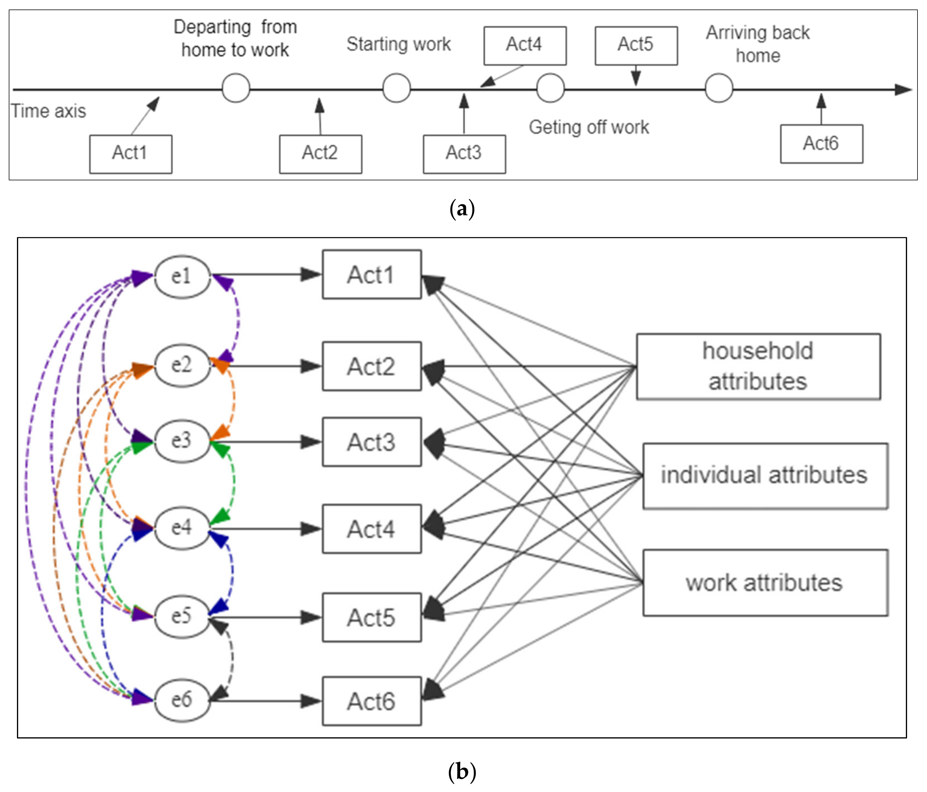
• Daily work time is a highly elastic factor for all types of outdoor non-work activity allocations of commuters. It has a positive effect on midday non-work activities (Act3 and Act4), but a negative effect on morning and evening non-work activities (Act1, Act2, Act5, and Act6). This suggests that increasing the total work hours may shift the demands for non-work activities from morning or evening to noon.
• A work schedule is a combination of times when a commuter starts and finishes his/her work. The starting time for work has a significant impact on non-work activities before work (i.e., Act1 and Act2), while the off-work time has a significant impact on non-work activities after work (i.e., Act5 and Act6).
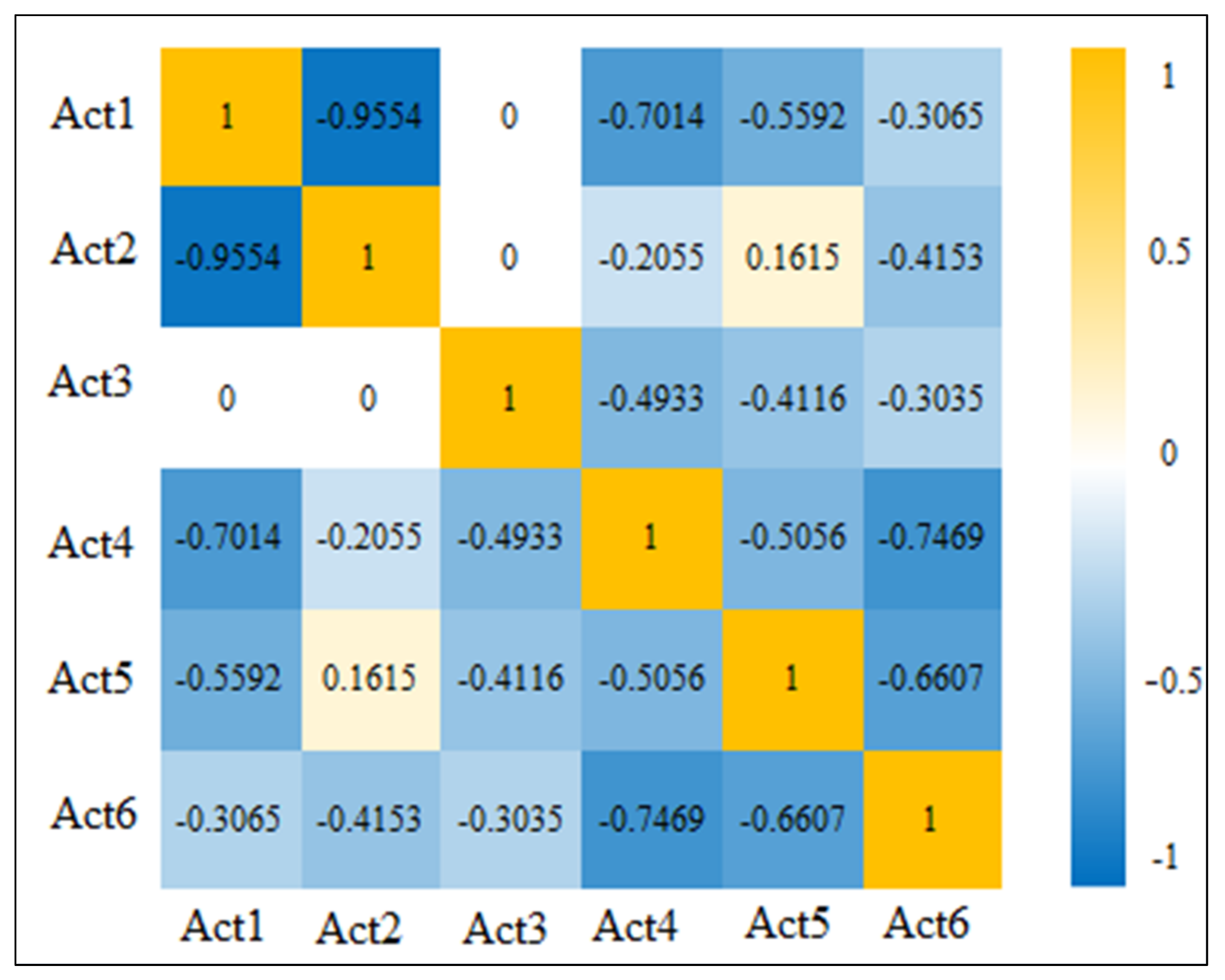
• The relation between Act2 and Act5 is mutually promotive, and the others are mutually substitutive. Some policies, like encouraging people to participate in activities during off-peak hours, may help to shift travel demand from peak hours to off-peak hours. It should be noted that the magnitude of error correlation depends on the number of significant variables being specified into the model. Model practitioners need to make extensive effort to screen and specify observed variables into the joint model in order to better control their effects and capture correlations among unspecified attributes truly reflecting inherent factors affecting activity or travel behaviours.
• When trip chains become increasingly complex, commuters will be more likely to use motorized private modes, such as automobiles. This indicates that the level of motorization in Xiaoshan District may continue to increase in the future. Local transportation authority should formulate some reasonable policies to prevent traffic congestion.

Some empirical results are consistent with previous findings. Self-employed commuters are more likely to undertake Act2 activities, while walking commuters are more reluctant to undertake Act5 activities, which is consistent with the finding in Wu and Ye [7]. What’s more, Act2 and Act5 are mutually promotive, which is also consistent with the finding of Wu and Ye [7] from Xiamen, China. This indicates that the conclusion may be universal and can be regionally transferred in similar areas.

However, the conclusions may only be applied to developed regions in developing countries like Xiaoshan District of China, whose universality is uncertain. Accordingly, the empirical results can be compared with the estimated results from other cities in different countries, if possible, in future work. This study reveals that there exist both substitutive and promotive relationships among various types of outdoor non-work activities. Future research can be focused on investigating the universality of the relationships and reasons behind it. After understanding the reasons, we will be able to put forward more accurate and efficient suggestions for the local government to improve local transportation system. Some new modeling methods, such as the multivariate heterogeneous-dispersion count model, the multivariate ordered probit regression model, and so on [35,42,43], may be employed to estimate similar multivariate choice models to further explore inherent relationships among non-work activity allocations. Furtherly, estimated results from different models can be compared to see the goodness-of-fit of different models.

References

1. Shanghai Urban and Rural Construction and Transportation Development Research Institute. The Fifth Comprehensive Traffic Survey in Shanghai; Shanghai Urban and Rural Construction and Transportation Development Research Institute: Shanghai, China, 2015. [Google Scholar]
2. Dissanayake, D.; Morikawa, T. Household travel behavior in developing countries: Nested logit model of vehicle ownership, mode choice, and trip chaining. Transp. Res. Rec. 2002, 1805, 45–52. [Google Scholar] [CrossRef]
3. Bhat, C.R. Work travel mode choice and number of non-work commute stops. Transp. Res. Part B Methodol. 1997, 31, 41–54. [Google Scholar] [CrossRef] [Green Version]
4. Vickerman, R. The demand for non-work travel. J. Transp. Econ. Policy 1972, 6, 176–210. [Google Scholar]
5. Maat, K.; Van Wee, B.; Stead, D. Land use and travel behaviour: Expected effects from the perspective of utility theory and activity-based theories. Environ. Plan. B Plan. Des. 2005, 32, 33–46. [Google Scholar] [CrossRef]
6. Manoj, M.; Verma, A. Activity-travel behaviour of non-workers belonging to different income group households in Bangalore, India. J. Transp. Geogr. 2015, 49, 99–109. [Google Scholar] [CrossRef]
7. Wu, Z.; Ye, X. Joint modeling analysis of trip-chaining behavior on round-trip commute in the context of Xiamen, China. Transp. Res. Rec. 2008, 2076, 62–69. [Google Scholar] [CrossRef]
8. Bhat, C. An analysis of evening commute stop-making behavior using repeated choice observations from a multi-day survey. Transp. Res. Part B Methodol. 1999, 33, 495–510. [Google Scholar] [CrossRef] [Green Version]
9. Bhat, C.R.; Sardesai, R. The impact of stop-making and travel time reliability on commute mode choice. Transp. Res. Part B Methodol. 2006, 40, 709–730. [Google Scholar] [CrossRef] [Green Version]
10. Cao, X.; Mokhtarian, P.L.; Handy, S.L. Differentiating the influence of accessibility, attitudes, and demographics on stop participation and frequency during the evening commute. Environ. Plan. B Plan. Des. 2008, 35, 431–442. [Google Scholar] [CrossRef]
11. Currie, G.; Delbosc, A. Exploring the trip chaining behaviour of public transport users in Melbourne. Transp. Policy 2011, 18, 204–210. [Google Scholar] [CrossRef]
12. Portoghese, A.; Spissu, E.; Bhat, C.R.; Eluru, N.; Meloni, I. A copula-based joint model of commute mode choice and number of non-work stops during the commute. Int. J. Transp. Econ. Riv. Internazionale Econ. Trasp. 2011, 38, 337–362. [Google Scholar]
13. Susilo, Y.O.; Kitamura, R. Structural changes in commuters’ daily travel: The case of auto and transit commuters in the Osaka metropolitan area of Japan, 1980–2000. Transp. Res. Part A Policy Pract. 2008, 42, 95–115. [Google Scholar] [CrossRef]
14. Li, W.; Li, Y.; Ban, X.; Deng, H.; Shu, H.; Xie, D. Exploring the Relationships between the Non-Work Trip Frequency and Accessibility Based on Mobile Phone Data. Transp. Res. Rec. 2018, 2672, 91–102. [Google Scholar] [CrossRef]
15. Mao, Z.; Ettema, D.; Dijst, M. Analysis of travel time and mode choice shift for non-work stops in commuting: Case study of Beijing, China. Transportation 2018, 45, 751–766. [Google Scholar] [CrossRef]
16. Brunow, S.; Gründer, M. The impact of activity chaining on the duration of daily activities. Transportation 2013, 40, 981–1001. [Google Scholar] [CrossRef]
17. Levinson, D.; Kumar, A. Activity, travel, and the allocation of time. J. Am. Plan. Assoc. 1995, 61, 458–470. [Google Scholar] [CrossRef]
18. Hunt, J.D.; Patterson, D. A stated preference examination of time of travel choice for a recreational trip. J. Adv. Transp. 1996, 30, 17–44. [Google Scholar] [CrossRef]
19. Sultana, S. Mode and Departure Time Choice Behavior of Non-Work Related Trips. Master’s Thesis, Schulich School of Engineering, Calgary, AB, Canada, 2019. [Google Scholar]
20. Khan, S.; Maoh, H.; Lee, C.; Anderson, W. Toward sustainable urban mobility: Investigating nonwork travel behavior in a sprawled Canadian city. Int. J. Sustain. Transp. 2016, 10, 321–331. [Google Scholar] [CrossRef]
21. Walle, S.V.; Steenberghen, T. Space and time related determinants of public transport use in trip chains. Transp. Res. Part A Policy Pract. 2006, 40, 151–162. [Google Scholar] [CrossRef]
22. Hensher, D.A.; Reyes, A.J. Trip chaining as a barrier to the propensity to use public transport. Transportation 2000, 27, 341–361. [Google Scholar] [CrossRef]
23. Ye, X.; Pendyala, R.M.; Gottardi, G. An exploration of the relationship between mode choice and complexity of trip chaining patterns. Transp. Res. Part B Methodol. 2007, 41, 96–113. [Google Scholar] [CrossRef] [Green Version]
24. Ma, C.; He, R.; Zhang, W. Path optimization of taxi carpooling. PLoS ONE 2018, 13, e0203221. [Google Scholar] [CrossRef] [PubMed]
25. Tang, J.; Liang, J.; Zhang, S.; Huang, H.; Liu, F. Inferring driving trajectories based on probabilistic model from large scale taxi GPS data. Phys. A Stat. Mech. Its Appl. 2018, 506, 566–577. [Google Scholar] [CrossRef]
26. Ma, C.; Hao, W.; Wang, A.; Zhao, H. Developing a coordinated signal control system for urban ring road under the vehicle-infrastructure connected environment. IEEE Access 2018, 6, 52471–52478. [Google Scholar] [CrossRef]
27. Tang, J.; Liang, J.; Han, C.; Li, Z.; Huang, H. Crash injury severity analysis using a two-layer Stacking framework. Accid. Anal. Prev. 2019, 122, 226–238. [Google Scholar] [CrossRef]
28. Zou, Y.; Ash, J.E.; Park, B.-J.; Lord, D.; Wu, L. Empirical Bayes estimates of finite mixture of negative binomial regression models and its application to highway safety. J. Appl. Stat. 2018, 45, 1652–1669. [Google Scholar] [CrossRef]
29. Zou, Y.; Zhong, X.; Tang, J.; Ye, X.; Wu, L.; Ijaz, M.; Wang, Y. A Copula-Based Approach for Accommodating the Underreporting Effect in Wildlife‒Vehicle Crash Analysis. Sustainability 2019, 11, 418. [Google Scholar] [CrossRef]
30. Zhang, R.; Ye, X.; Wang, K.; Li, D.; Zhu, J. Development of commute mode choice model by integrating actively and passively collected travel data. Sustainability 2019, 11, 2730. [Google Scholar] [CrossRef]
31. Ye, X.; Wang, K.; Zou, Y.; Lord, D. A semi-nonparametric Poisson regression model for analyzing motor vehicle crash data. PloS ONE 2018, 13, e0197338. [Google Scholar] [CrossRef]
32. Daisy, N.S.; Habib, M.A. Investigating the Role of Built Environment and Lifestyle Choices in Active Travel for Weekly Home-Based Nonwork Trips. Transp. Res. Rec. 2015, 2500, 125–132. [Google Scholar] [CrossRef]
33. Parady, G.T.; Chikaraishi, M.; Takami, K.; Ohmori, N.; Harata, N. On the effect of the built environment and preferences on non-work travel: Evidence from Japan. Eur. J. Transport. Infrastruct. Res. 2015, 15, 51–66. [Google Scholar]
34. Chib, S.; Greenberg, E. Analysis of multivariate probit models. Biometrika 1998, 85, 347–361. [Google Scholar] [CrossRef] [Green Version]
35. Cappellari, L.; Jenkins, S.P. Multivariate probit regression using simulated maximum likelihood. Stata J. 2003, 3, 278–294. [Google Scholar] [CrossRef]
36. Börsch-Supan, A.; Hajivassiliou, V.A. Smooth unbiased multivariate probability simulators for maximum likelihood estimation of limited dependent variable models. J. Econom. 1993, 58, 347–368. [Google Scholar] [CrossRef] [Green Version]
37. Borsch-Supan, A.; Hajivassiliou, V.; Kotlikoff, L.J. Health, children, and elderly living arrangements: A multiperiod-multinomial probit model with unobserved heterogeneity and autocorrelated errors. In Topics in the Economics of Aging; University of Chicago Press: Chicago, IL, USA, 1992; pp. 79–108. [Google Scholar]
38. Hajivassiliou, V.A.; Ruud, P.A. Classical estimation methods for LDV models using simulation. Handb. Econom. 1994, 4, 2383–2441. [Google Scholar]
39. Bhat, C.R.; Sidharthan, R. A new approach to specify and estimate non-normally mixed multinomial probit models. Transp. Res. Part B Methodol. 2012, 46, 817–833. [Google Scholar] [CrossRef] [Green Version]
40. Ma, J.; Ye, X.; Shi, C. Development of Multivariate Ordered Probit Model to Understand Household Vehicle Ownership Behavior in Xiaoshan District of Hangzhou, China. Sustainability 2018, 10, 3660. [Google Scholar] [CrossRef]
41. Bhat, C.R.; Varin, C.; Ferdous, N. A comparison of the maximum simulated likelihood and composite marginal likelihood estimation approaches in the context of the multivariate ordered-response model. In Maximum Simulated Likelihood Methods and Applications; Emerald Group Publishing Limited: Bingley, UK, 2010; pp. 65–106. [Google Scholar]
42. Mothafer, G.I.; Yamamoto, T.; Shankar, V.N. A multivariate heterogeneous-dispersion count model for asymmetric interdependent freeway crash types. Transp. Res. Part B Methodol. 2018, 108, 84–105. [Google Scholar] [CrossRef]
43. Bhat, C.R. New matrix-based methods for the analytic evaluation of the multivariate cumulative normal distribution function. Transp. Res. Part B Methodol. 2018, 109, 238–256. [Google Scholar] [CrossRef]
44. Godambe, V.P. An optimum property of regular maximum likelihood estimation. Ann. Math. Stat. 1960, 31, 1208–1211. [Google Scholar] [CrossRef]
45. Zhao, Y.; Joe, H. Composite likelihood estimation in multivariate data analysis. Can. J. Stat. 2005, 33, 335–356. [Google Scholar] [CrossRef]
Figure 1. The modeling framework. (a) The timeline of a commuter’s daily activities; (b) Simplified modeling framework.
Sustainability 11 05768 g001
Figure 2. Map of Hangzhou and Xiaoshan with district divisions.
Sustainability 11 05768 g002
Figure 3. Estimated error correlation matrix.
Sustainability 11 05768 g003