A Method to Assess and Reduce Pollutant Emissions of Logistic Transportation under Adverse Weather

Abstract
:1. Introduction
2. Problem and Methods
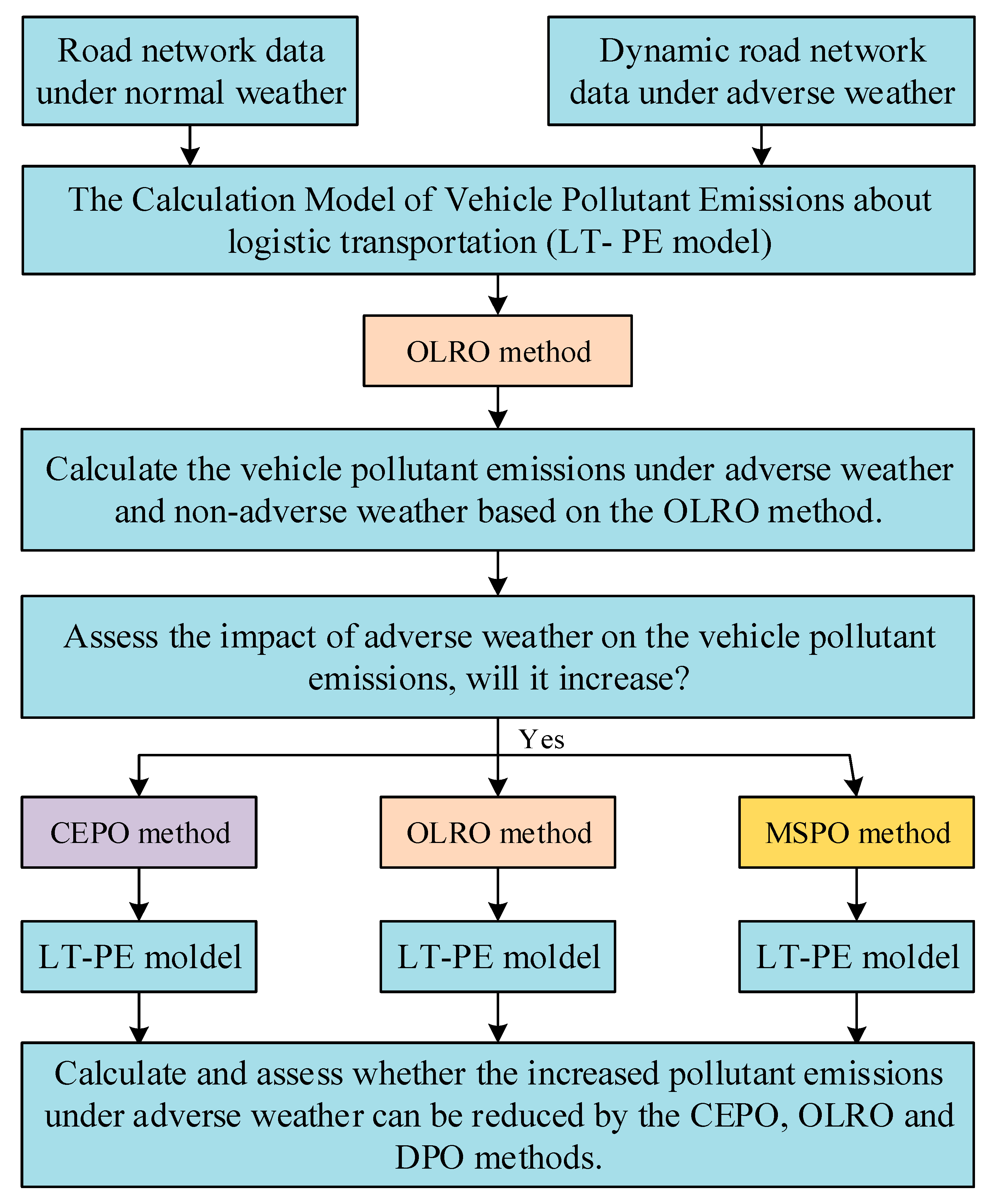
2.1. Methodological Framework
2.2. Calculation Model of Vehicle Pollutant Emissions
2.3. Mathematical Descriptions of MSPO, OLRO, and CEPO
2.4. The Realization of CEPO
3. Case study
3.1. Fruit Transportation in Hainan Island
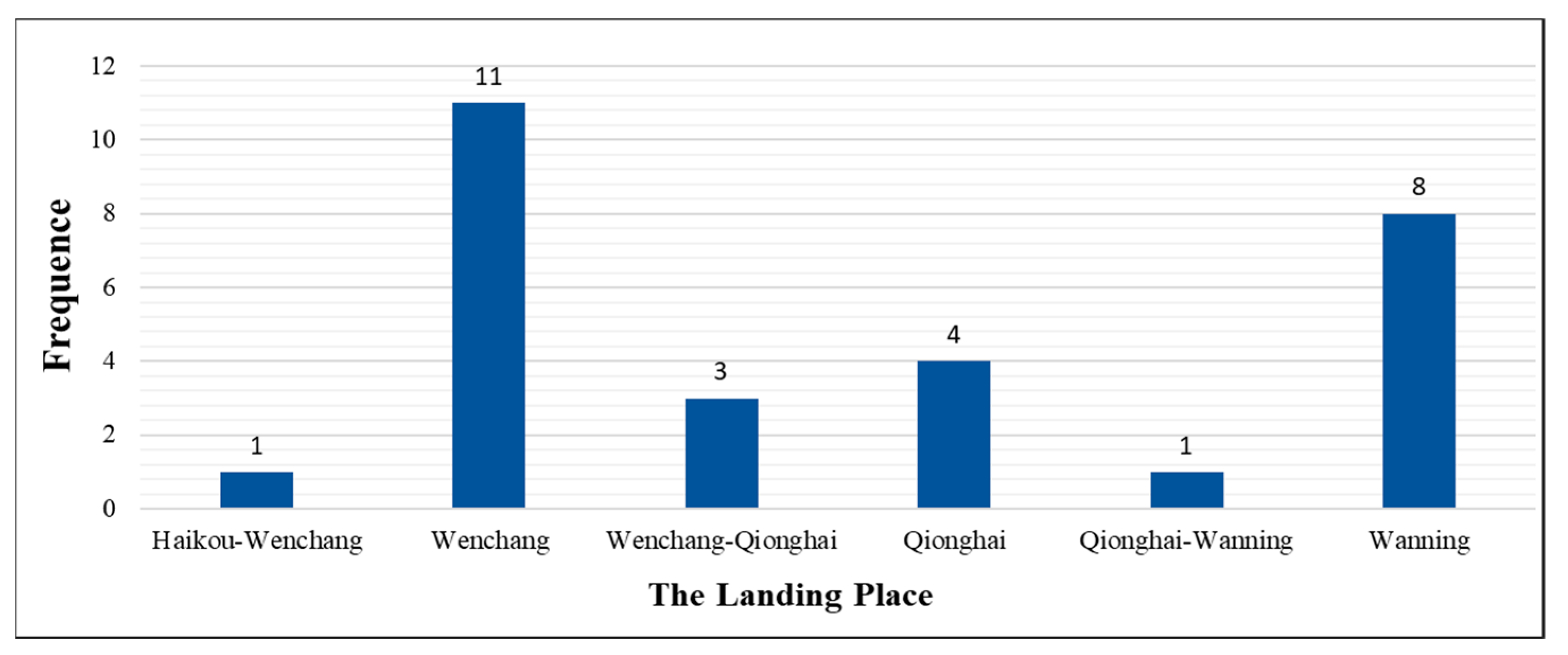
3.2. Adverse Weather Condition—Typhoon
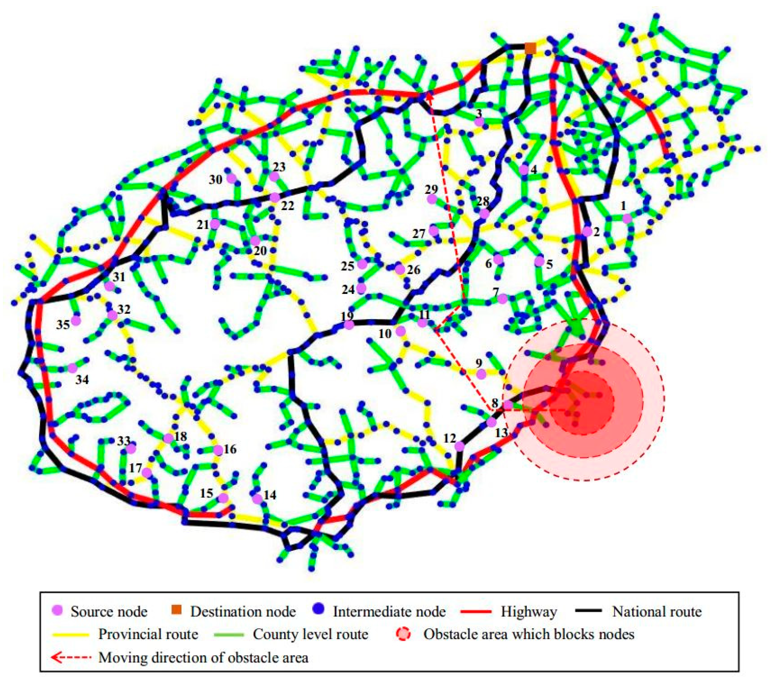
3.3. Route Network System
3.4. Determination of Emission Factors (F)
4. Simulation and Results
4.1. Experiment Setup
4.2. Experiments to Verify Whether Vehicle Emissions Increase under Adverse Weather
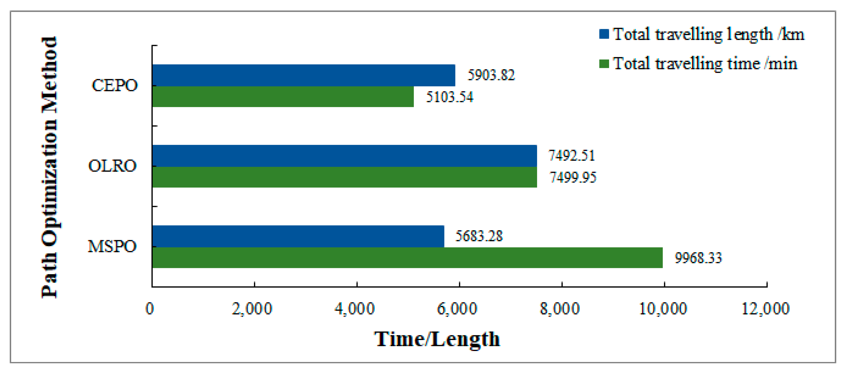
4.3. Comparative Experiment between Three Path Optimization Methods
5. Conclusions and Future Work
Author Contributions
Funding
Conflicts of Interest
References
- Yuan, Q. Location of Warehouses and Environmental Justice. J. Plan. Educ. Res. 2018, 1–12. [Google Scholar] [CrossRef]
- Souleymane, C.; Klaus, D.U. World Development Report 2009: Reshaping the World Boundary Economic Geography; World Bank: Washington, DC, USA, 2009. [Google Scholar]
- UNEP. Annual Report of United Nations Enviroment Programme; UNEP: Nairobi, Kenya, 2010. [Google Scholar]
- Rice, M.B.; Rifas-Shiman, S.L.; Litonjua, A.A.; Oken, E.; Gillman, M.W.; Kloog, I. Lifetime Exposure to Ambient Pollution and Lung Function in Children. Am. J. Resp. Crit. Care Med. 2016, 193, 881–888. [Google Scholar] [CrossRef] [PubMed] [Green Version]
- Hsu, Y.H.; Chuang, H.C.; Lee, Y.H.; Lin, Y.F.; Chen, Y.J.; Hsiao, T.C.; Wu, M.Y.; Chiu, H.W. Traffic-related particulate matter exposure induces nephrotoxicity in vitro and In Vivo. Free Radic. Biol. Med. 2019, 135, 235–244. [Google Scholar] [CrossRef] [PubMed]
- Lei, Z.; Bo-Guang, W.; Da-Gang, T. Impact of Heavy-Duty Diesel Vehicles on Air Quality and Control of Their Emissions. Environ. Sci. 2011, 32, 2177–2183. [Google Scholar]
- Kerry, E. Increasing destructiveness of tropical cyclones over the past 30 years. Nature 2005, 436, 686–688. [Google Scholar]
- Giuliano, G.; O’Brien, T.; Dablanc, L.; Holliday, K. Synthesis of Freight Research in Urban Transportation Palnning; National Academy of Science: Washington, DC, USA, 2013. [Google Scholar]
- Wang, H.; Chen, C.; Huang, C. On-road vehicle emission inventory and its uncertainty analysis for Shanghai, China. Sci. Total Environ. 2008, 398, 60–67. [Google Scholar] [CrossRef]
- Frances, M. Climate Change and Air Pollution: Exploring the Synergies and Potential for Mitigation in Industrializing Countries. Sustainability 2009, 1, 43–54. [Google Scholar] [Green Version]
- NBSC. China Statistical Yearbook; China Statistical Publisher: Beijing, China, 2015. (In Chinese)
- Yang, F.; Yu, L.; Song, G. Application of small sampling approach to estimating vehicle mileage accumulations for Beijing. J. Transp. Res. Board 2005, 1, 77–82. [Google Scholar] [CrossRef]
- Peters, J.M. Epidemiologic Investigation to Identify Chronic Effects of Ambient Air Pollutants in Southern California; Department of Preventive Medicine, University of Southern California: Los Angeles, CA, USA, 2004. [Google Scholar]
- Giuliano, G.; Dessouky, M.; Moore, J.E., II. Selected Papers from the National Urban Freight Conference. Transp. Res. Part E 2008, 44, 181–184. [Google Scholar]
- Webster, P.J. Changes in Tropical Cyclone Number, Duration, and Intensity in a Warming Environment. Science 2005, 309, 1844–1846. [Google Scholar] [CrossRef] [Green Version]
- Fang, J.; Sun, S.; Shi, P. Assessment and Mapping of Potential Storm Surge Impacts on Global Population and Economy. Int. J. Disaster Risk Sci. 2014, 5, 323–331. [Google Scholar] [CrossRef] [Green Version]
- Gao, B.; Liu, W. Emissions reduction potential analysis of road transportation. Geogr. Res. 2013, 32, 767–775. (In Chinese) [Google Scholar]
- Klier, T.; Linn, J. Using Taxes to Reduce Carbon Dioxide Emissions Rates of New Passenger Vehicles: Evidence from France, Germany, and Sweden. SSRN Electron. J. 2015, 7, 212–242. [Google Scholar] [CrossRef]
- McKinnon, A.C. The Potential of Economic Incentives to Reduce CO2 Emissions from Cargo Transport. DILF Orienter. 2010, 47, 24–38. [Google Scholar]
- Subramaniyam, K.V.; Kumar, C.S.N.; Subramanian, S.C. Analysis of Handling Performance of Hybrid Electric Vehicles. IFAC-Pap 2018, 51, 190–195. [Google Scholar] [CrossRef]
- Nienhueser, I.A.; Qiu, Y. Economic and environmental impacts of providing renewable energy for electric vehicle charging–A choice experiment study. Appl. Energy 2016, 180, 256–268. [Google Scholar] [CrossRef]
- Igliński, H.; Babiak, M. Analysis of the Potential of Autonomous Vehicles in Reducing the Emissions of Greenhouse Gases in RouteTransport. Procedia Eng. 2017, 192, 353–358. [Google Scholar] [CrossRef]
- Sternab, R.E.; Chen, Y.C.; Churchill, M. Quantifying air quality benefits resulting from few autonomous vehicles stabilizing traffic. Transp. Res. Part D Transp. Environ. 2019, 67, 351–365. [Google Scholar] [CrossRef]
- Shancita, I.; Masjuki, H.H.; Kalam, M.A.; Rizwanul Fattah, I.M.; Rashed, M.M.; Rashedul, H.K. A review on idling reduction strategies to improve fuel economy and reduce exhaust emissions of transport vehicles. Energy Convers. Manag. 2014, 88, 794–807. [Google Scholar] [CrossRef]
- Stevanovic, A.; Stevanovic, J.; Zhang, K.; Batterman, S. Optimizing traffic control to reduce fuel consumption and vehicular emissions: Integrated approach with VISSIM, CMEM, and VISGAOST. J. Transp. Res. Board 2009, 2128, 105–113. [Google Scholar] [CrossRef]
- Barth, M.J.; Wu, G.Y.; Boriboonsomsin, K. Intelligent Transportation Systems and Greenhouse Gas Reductions. Curr. Sustain./Renew. Energy Rep. 2015, 2, 1–8. [Google Scholar] [CrossRef]
- Soon, K.L.; Lim, J.M.Y.; Parthiban, R. Coordinated Traffic Light Control in Cooperative Green Vehicle Routing for Pheromone-based Multi-Agent Systems. Appl. Soft Comput. 2019, 81, 105486. [Google Scholar] [CrossRef]
- Organ, B.; Huang, Y.; Zhou, J.L.; Surawski, N.C.; Yam, Y.S.; Mok, W.C.; Hong, G. A remote sensing emissions monitoring programme reduces emissions of gasoline and LPG vehicles. Environ. Res. 2019, 177, 108614. [Google Scholar] [CrossRef] [PubMed]
- Savković, T.; Miličić, M.; Pitka, P.; Milenković, I.; Koleška, D. Evaluation of the eco-driving training of professional truck drivers. Oper. Res. Eng. Sci. Theory Appl. 2019, 2, 15–26. [Google Scholar] [CrossRef]
- Barth, M.; Boriboonsomsin, K. Energy and emissions impacts of a freeway-based dynamic eco-driving system. Transp. Res. Part D Transp. Environ. 2009, 14, 400–410. [Google Scholar] [CrossRef]
- Frigioni, D.; Marchetti-Spaccamela, A.; Nanni, U. Fully dynamic algorithms for maintaining shortest paths trees. J. Algorithms 2000, 34, 251–281. [Google Scholar] [CrossRef]
- Frigioni, D.; Marchetti-Spaccamela, A.; Nanni, U. Semidynamic algorithms for maintaining single-source shortest path trees. Algorithm Mica 1998, 22, 250–274. [Google Scholar] [CrossRef]
- Ding, W.; Qiu, K. Incremental single-source shortest paths in digraphs with arbitrary positive arc weights. Theor. Comput. Sci. 2017, 674, 16–31. [Google Scholar] [CrossRef]
- Narvaez, K.S.; Tzeng, H. New dynamic algorithms for shortest path tree computation. IEEE/ACM Trans. Netw. 2000, 8, 734–746. [Google Scholar] [CrossRef]
- Idri, A.; Oukarfi, M.; Boulmakoul, A.; Zeitouni, K.; Masri, A. A distributed approach for shortest path algorithm in dynamic multimodal transportation networks. Transp. Res. Procedia 2017, 27, 294–300. [Google Scholar] [CrossRef]
- Ramalingam, G.; Reps, T. An incremental algorithm for a generalization of the shortest-path problem. J. Algorithm 1996, 21, 267–305. [Google Scholar] [CrossRef]
- Sheng, Y.; Gao, Y. Shortest path problem of uncertain random network. Comput. Ind. Eng. 2016, 99, 97–105. [Google Scholar] [CrossRef]
- Baue, R.; Wagner, D. Batch dynamic single-source shortest-path algorithms: An experimental study. Exp. Algorithms 2009, 5526, 51–62. [Google Scholar]
- Taoka, D.; Takafuji, T.; Watanabe, T.I. Performance comparison of algorithms for the dynamic shortest path problem. IEICE Transactions on Fundamentals of Electronics. Commun. Comput. Sci. 2007, 847, 847–2007. [Google Scholar]
- Paul, B. Rerouting shortest paths in planar graphs. Discret. Appl. Math. 2017, 231, 95–112. [Google Scholar] [Green Version]
- Hu, X.B.; Zhang, M.K.; Zhang, Q.; Liao, J.Q. Co-evolving path Optimization by Ripple-Spreading Algorithm. Transp. Res. Part B Methodol. 2017, 106, 411–432. [Google Scholar] [CrossRef]
- Hu, X.B.; Wang, M.; Leeson, M.S.; Hines, E.L.; Di Paolo, E. Deterministic Agent-Based Path Optimization Method by Mimicking the Spreading of Ripples. Evol. Comput. 2016, 24, 319–346. [Google Scholar] [CrossRef]
- Xie, R.F.; Chen, Z.B.; Deng, X.K. Characteristics of Motor Vehicle Pollutant Emission and Share Ratio in Haikou City Based on MOVES2014a. Nat. Sci. J. Hainan Univ. 2017, 35, 87–94. (In Chinese) [Google Scholar]
- Hu, X.B.; Wang, M.; Hu, D.; Leeson, M.S.; Hines, E.L.; Di Paolo, E. A Ripple-Spreading Algorithm for the k Shortest Paths Problem. In Proceedings of the 2012 the 3rd Global Congress on Intelligent Systems, Wuhan, China, 6–8 November 2012; pp. 202–208. [Google Scholar]
- Hu, X.B.; Sun, Q.; Wang, M.; Leeson, M.S.; Hines, E.L.; Di Paolo, A. Ripple-Spreading Algorithm to Calculate the k Best Solutions to the Project Time Management Problem. In Proceedings of the 2013 IEEE Symposium Series on Computational Intelligence (IEEE SSCI 2013), Singapore, 16–19 April 2013. [Google Scholar]
- Deng, C.; Zhang, X.Q.; Liu, Y. Status analysis and development strategy of Harbor logistics industry in Hainan. Humanit. Soc. Sci. J. Hainan Univ. 2012, 30, 124–130. (In Chinese) [Google Scholar]
- Kunkel, K.E.; Easterling, D.R.; Kristovich, D.A.; Gleason, B.; Stoecker, L.; Smith, R. Recent increases in U.S. heavy precipitation associated with tropical cyclones. Geophys. Res. Lett. 2010, 37, 701–719. [Google Scholar] [CrossRef]
- Malmstadt, J.C.; Elsner, J.B.; Jagger, T.H. Risk of strong hurricane winds to Florida cities. J. Appl. Meteor. Clim. 2010, 49, 2121–2132. [Google Scholar] [CrossRef]
- China Meteorological Administration, Grade of Weather Conditions for Freeway Transportation; China Meteorological Press: Beijing, China, 2010.


| Types of Motor Vehicles | CO | HC | NOx | Tv | |
|---|---|---|---|---|---|
| Displacement > l liter | Light diesel vehicles | 1.682 | 0.428 | 1.12 | 1 |
| Medium-sized diesel vehicles | 2.268 | 0.428 | 3.48 | 2 | |
| Heavy duty diesel vehicle | 3.823 | 0.742 | 5.882 | 3 | |
| Farm Number | Farm Name | No Typhoon | Typhoon | |||||
|---|---|---|---|---|---|---|---|---|
| PL/km | TT/h | PE/g | PL/km | TT/h | PE/g | |||
| Farms whose fruit transpor-tation is not affected by typhoon | 1 | Sanjiaoting | 92.07 | 1.63 | 1833.71 | 92.07 | 1.63 | 1833.71 |
| 3 | Jinan | 48.31 | 1.00 | 962.15 | 48.31 | 1.00 | 962.15 | |
| 4 | Jinjiling | 57.16 | 1.03 | 1138.51 | 57.16 | 1.03 | 1138.51 | |
| 7 | Dongtai | 133.87 | 2.50 | 2666.16 | 134.97 | 3.05 | 2688.05 | |
| 8 | Xinglong | 163.57 | 2.06 | 3247.33 | 163.57 | 2.06 | 3247.33 | |
| 9 | Xinzhong | 176.37 | 2.51 | 3512.73 | 176.37 | 2.51 | 3512.73 | |
| 12 | Lingmen | 186.38 | 2.52 | 3712.05 | 186.38 | 2.52 | 3712.05 | |
| 13 | Nanlin | 172.03 | 2.28 | 3426.21 | 172.03 | 2.28 | 3426.21 | |
| 14 | Nandao | 289.59 | 3.98 | 5767.63 | 289.59 | 3.98 | 5767.63 | |
| 16 | Baoguo | 317.33 | 4.47 | 6320.11 | 317.33 | 4.47 | 6320.11 | |
| 21 | Zhubijiang | 179.75 | 2.93 | 3580.04 | 179.75 | 2.93 | 3580.04 | |
| 31 | Hongquan | 195.82 | 2.75 | 3900.02 | 195.82 | 2.75 | 3900.02 | |
| 34 | Gongai | 246.21 | 3.36 | 4887.93 | 246.21 | 3.36 | 4887.93 | |
| 35 | Datian | 232.34 | 3.26 | 4627.43 | 232.34 | 3.26 | 4627.43 | |
| Farms whose fruit transpor-tation is affected by typhoon | 2 | Donghong | 77.44 | 1.05 | 1542.33 | 89.25 | 1.46 | 1777.51 |
| 5 | Zhongrui | 109.30 | 1.89 | 2176.97 | 113.85 | 1.95 | 2267.54 | |
| 6 | Zhongjian | 100.02 | 1.89 | 1985.64 | 109.79 | 2.38 | 2179.59 | |
| 10 | Nanfeng | 140.33 | 2.43 | 2794.92 | 211.05 | 3.38 | 4203.36 | |
| 11 | Lingtou | 147.41 | 2.70 | 2926.61 | 225.57 | 3.05 | 4478.15 | |
| 15 | Licai | 299.00 | 4.01 | 5936.12 | 358.51 | 6.71 | 7117.42 | |
| 17 | Jiusuo | 312.43 | 4.56 | 6202.62 | 476.52 | 8.92 | 9460.44 | |
| 18 | Leguang | 236.98 | 4.67 | 4704.71 | 452.14 | 8.47 | 8976.27 | |
| 19 | Xinwei | 152.48 | 2.60 | 3027.09 | 230.63 | 2.97 | 4578.63 | |
| 20 | Weixing | 159.79 | 3.07 | 3172.27 | 177.17 | 3.19 | 3517.39 | |
| 22 | Xipei | 137.87 | 2.44 | 2737.20 | 155.26 | 2.90 | 3082.32 | |
| 23 | Xiqing | 140.20 | 2.63 | 2783.33 | 157.58 | 2.94 | 3128.44 | |
| 24 | Dafeng | 134.19 | 2.71 | 2664.06 | 175.92 | 3.29 | 3492.44 | |
| 25 | Yangjiang | 135.96 | 2.70 | 2699.12 | 172.31 | 3.22 | 3420.96 | |
| 26 | Xinjin | 120.15 | 2.31 | 2385.31 | 346.17 | 6.48 | 6872.49 | |
| 27 | Huangling | 109.05 | 2.08 | 2165.01 | 333.29 | 6.24 | 6616.88 | |
| 28 | Guangqing | 74.82 | 1.31 | 1485.36 | 114.73 | 1.44 | 2277.72 | |
| 29 | Chenxing | 94.97 | 2.08 | 1885.37 | 180.89 | 3.11 | 3591.2 | |
| 30 | Xihua | 157.56 | 2.90 | 3138.02 | 174.94 | 4.31 | 3473.13 | |
| 32 | Guangba | 241.55 | 3.43 | 4795.49 | 380.87 | 4.99 | 7561.44 | |
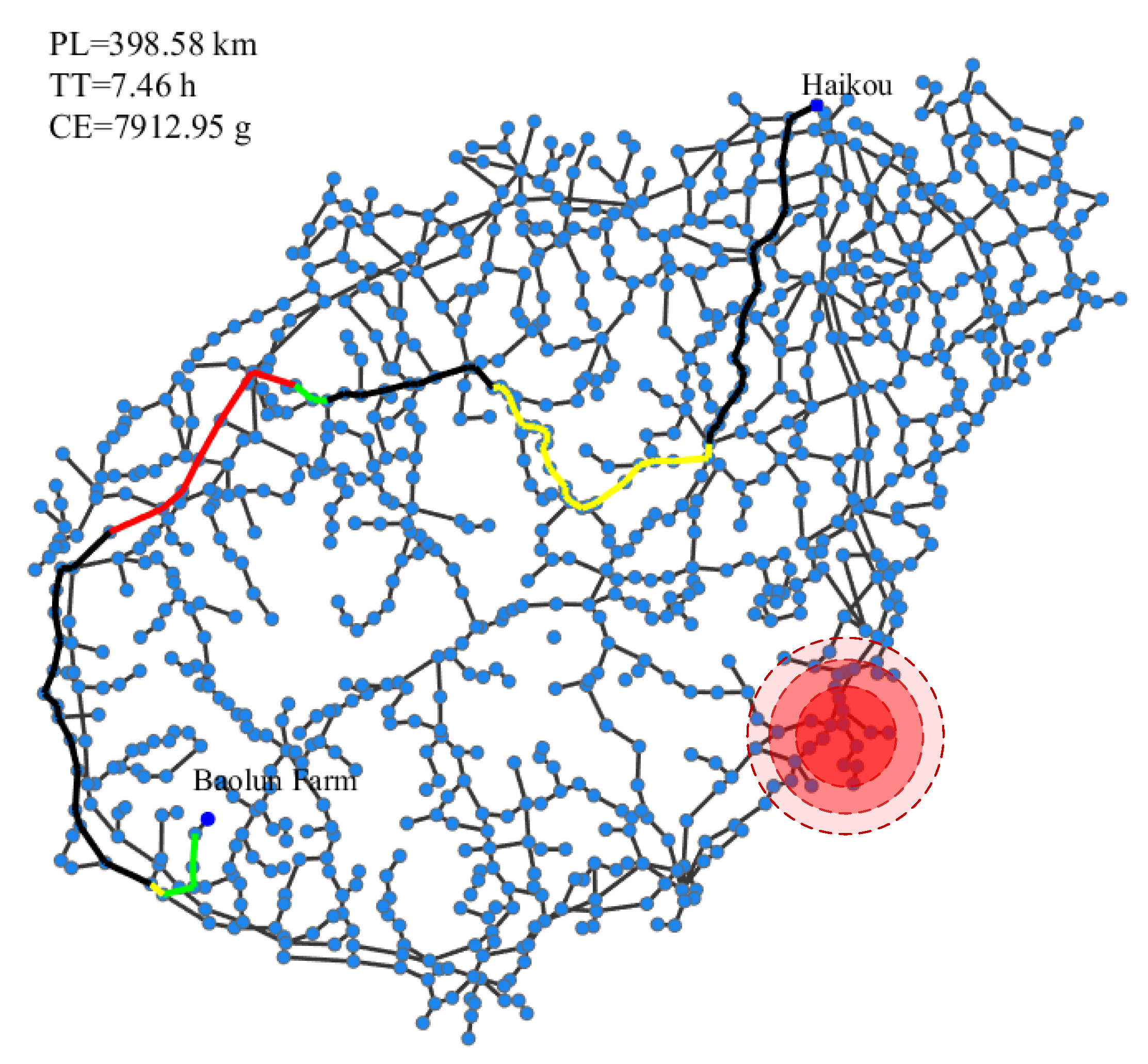
| 33 | Baolun | 325.90 | 5.03 | 6470.19 | 398.58 | 7.42 | 7913.01 | |
| SUM | 5898.19 | 94.8 | 117,471.3 | 7725.69 | 130.2 | 153,868.7 | ||
© 2019 by the authors. Licensee MDPI, Basel, Switzerland. This article is an open access article distributed under the terms and conditions of the Creative Commons Attribution (CC BY) license (http://creativecommons.org/licenses/by/4.0/).
Share and Cite
Zhang, M.; Hu, X.; Wang, J. A Method to Assess and Reduce Pollutant Emissions of Logistic Transportation under Adverse Weather. Sustainability 2019, 11, 5961. https://doi.org/10.3390/su11215961
Zhang M, Hu X, Wang J. A Method to Assess and Reduce Pollutant Emissions of Logistic Transportation under Adverse Weather. Sustainability. 2019; 11(21):5961. https://doi.org/10.3390/su11215961
Chicago/Turabian StyleZhang, Mingkong, Xiaobing Hu, and Jingai Wang. 2019. "A Method to Assess and Reduce Pollutant Emissions of Logistic Transportation under Adverse Weather" Sustainability 11, no. 21: 5961. https://doi.org/10.3390/su11215961