Restricted Airspace Unit Identification Using Density-Based Spatial Clustering of Applications with Noise

Abstract

This paper first calculates the departure delay and arrival delay of each flight by mining historical flight data. Then, a new method based on density clustering for identification and visualization of restricted airspace units that considers this activity is proposed. The main objective is to identify the restricted airspace units by calculating the average delay time according to the accumulative delay time of airspace units and the accumulative delay flight. Therefore, the density-based spatial clustering of applications with noise (DBSCAN) clustering method is utilized to match the latitude and longitude coordinates of each spatial domain unit with its delay time to construct a feature matrix, and then clustering analysis is conducted according to the time period. The method aims at identifying the most severe restricted units in each period. The reliability and applicability of the proposed method are validated through a real case study with flight information from Beijing Capital International Airport, Hongqiao International Airport, and Baiyun International Airport during a typical day. The investigation shows that the DBSCAN clustering method can identify the restricted spatial units intuitively on the six flight paths between Beijing Capital International Airport, Hongqiao International Airport, and Baiyun International Airport.

1. Introduction

With the continuous growth of China’s air traffic volume, the problem of flight delays has become a major bottleneck restricting the rapid development of civil aviation. Flight delays are difficult to avoid, and as the flight delays accumulate, the risk of hidden dangers increases. There are many factors that cause flight delays in actual operation, such as airline operation management, bad weather, military activities and air traffic control, and so on. These factors will cause airspace units to be restricted to varying degrees, resulting in flight delays. The emergence and occurrence of these influencing factors are strongly random and uncertain. When these factors, such as bad weather, suddenly appear on the route, even if there are no restrictions within the airport and near the airport, it will cause one or more airspace units on the route to be restricted, causing delays in the flight. Moreover, delays of the previous flights may also lead to subsequent flight delays, so flight delay presents a chaotic or nonlinear development trend, and it is difficult to accurately predict flight delays. In this paper, restricted airspace units refer to the airspace units whose capacity and service level decrease because of weather and military activities. How to identify restricted airspace units in airspace and identify the starting and ending times of the restriction is important. It is also important to analyze the propagation mechanism of flight delays in depth and analyze the impact of a flight delay on subsequent flights. This analysis can also further improve the accuracy of flight delay prediction.

Over the years, a large quantity of research has been carried out in terms of flight delay prediction. There are mainly three kinds of research methods, namely, prediction methods based on statistical inference, simulation modeling, and machine learning. The flight delay prediction method based on statistical inference establishes a statistical model through statistical theory using actual sample data (mainly historical data). It further predicts flight delay time by analyzing data characteristics and estimating the characteristics of the sample data. Sridhar et al. conducted a study on short-term flight delay prediction methods [1]. They selected the Weather Impact Traffic Index (WITI), predicted WITI, and reference traffic volume as features, and they proposed a variety of linear autoregressive models. Klein et al. developed a multivariate regression model for airport delay prediction by using the Weather Impact Traffic Index (WITI). The model successfully predicted the time and extent of the effects of convective and non-convective weather throughout the year and the resulting delays [2]. In addition, Wu et al. established a Bayesian network model based on flight strings to simulate the relationship between flight delays. Their research revealed the impact of abnormal operating conditions on flight plan robustness [3]. Xu et al. developed an empirical Bayesian method to study how delays at the originating airport are transmitted to the destination airport [4]. Furthermore, Perez-Rodríguez et al. proposed an asymmetric Bayesian logit model to predict the daily delay probability of aircraft arrivals [5].

The flight delay prediction method based on simulation modeling characterizes some key variables of the flight operation system by simulating the operation of an aircraft in the aviation network. Through the simulation model (including aircraft operation model, delay propagation model, etc.) or simulation system, the variables are connected with the whole system to realize the prediction of aircraft delay time under different scenarios. In one study, Shao Yong constructed a complex network topology model with directed flights during a peak hour. The lateral wave effect of delayed flights in the airport and the longitudinal ripple effect between airports were analyzed in their research [6]. Moreover, Campanelli et al. introduced the TREE project (data-driven modeling of European Civil Aviation Commission (ECAC) regional response delay tree network extension) focusing on characterizing and predicting the propagation of reaction delays through European networks. A delay propagation tree model was developed to simulate the propagation of response delays in the ECAC region [7,8]. Shi et al. constructed a flight delay analysis model based on the uncertainty factor of colored time Petri nets. It clearly reflects the impact of uncertainties in flight operations on the spread of delays in order to predict the extent of delays [9]. Schaefer et al. used a detailed policy assessment tool (DPAT) to simulate delay propagation throughout the airport and sector systems [10]. Chen et al. utilized a Dynamic Data Driven Application System (DDDAS) for real-time forecasting of flight delays. A dynamic data-driven delay prediction framework was constructed based on the system state-space model [11]. Furthermore, National Aeronautics and Space Administration (NASA) and the Massachusetts Institute of Technology (MIT) have jointly built the scalable aeronautical network simulation system. It can assess air traffic capacity and service efficiency during weather changes, airport traffic changes, and airline decision changes [12].

The flight delay prediction method based on machine learning takes artificial intelligence as the theoretical basis and focuses on data-driven methodology. By mining a large amount of flight data, key features are extracted, then a machine learning model is established to predict the flight delay. Pfeil et al. demonstrated how to convert an original convective weather forecast, which provides a deterministic prediction of vertically integrated liquid (precipitation content in the air column), into the probability prediction of whether the route in the terminal area is blocked. Then, they applied a classification algorithm based on machine learning to determine the possibility of the route being used in actual weather conditions [13]. Moreover, Reboll et al. used a random forest algorithm to predict the direct delay over 2, 4, 6, and 24 h time intervals, then compared the prediction results with the regression model. Results showed that with the increase of time interval, the prediction accuracy will be reduced [14]. Choi et al. used data mining and supervised machine learning algorithms (random forest, decision tree, etc.) to predict airline flight delays caused by bad weather conditions [15]. Khanmohammadi used a multilevel input layer artificial neural network to predict flight delays at John F. Kennedy International Airport (JFK) [16]. Wu et al. proposed a flight delay prediction model, based on Spark and integrated meteorological data, and they used a parallelized random forest algorithm on Spark parallel computing architecture to generate the model [17]. Ding proposed a method of simulating flight arrivals and a multiple linear regression algorithm to predict delay, and when compared with the naive Bayes algorithm and C4.5 method, the prediction accuracy of the algorithm was further proved [18]. Furthermore, Choi et al. developed a delay prediction model for a single origin destination (OD) pair based on supervised machine learning algorithms with consideration of weather conditions [19].

Many scholars have done a lot of research in flight delay prediction. But, as mentioned above, flight delays are affected by many factors that have a certain suddenness and randomness. Therefore, flight delays appear to be chaotic or nonlinear and are difficult to predict accurately. At the same time, delay in one flight may also lead to subsequent flight delays. Although some scholars have consciously separated direct delays from delays caused by propagation, no effective method has been found to quantitatively distinguish the two. When an event causing a flight delay occurs, the airspace unit is restricted, causing flight delays. Identification of the restricted airspace unit and the start and end times of the restriction can help to solve the randomness of events caused by bad weather, air traffic control, and so on. Determining the start and end times of the restriction can separate direct delays from delays caused by propagation, enabling further exploration of the propagation mechanism of flight delays, which is of great significance for improving the accuracy of flight delay prediction.

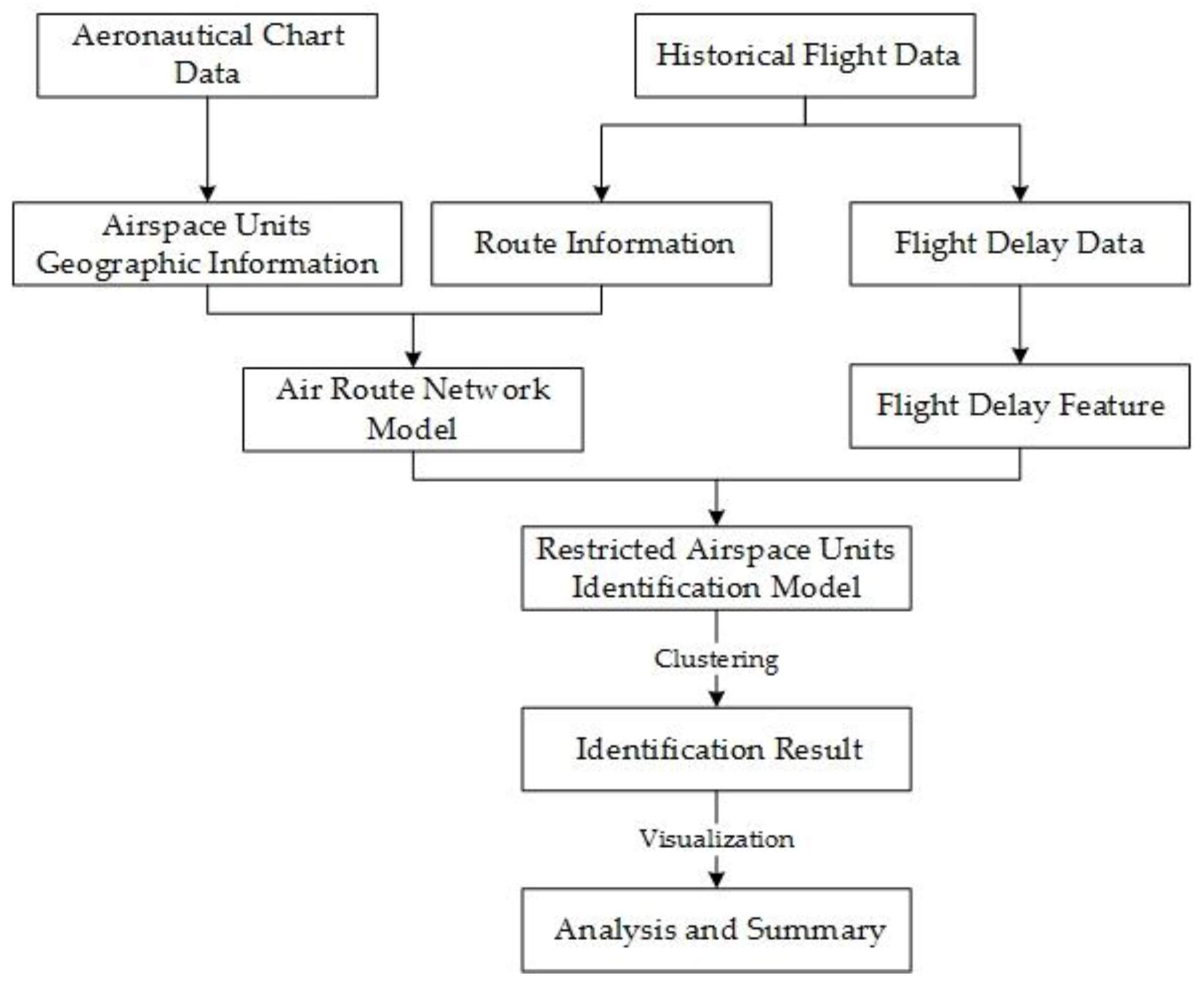
Firstly, in order to identify restricted units in the airspace, a definition of the airspace unit must be defined. In this study, the unit refers to the airport and the point on the airway. Secondly, the algorithm used to identify the restricted airspace unit needs to be determined. The identification can be regarded as a clustering process. Therefore, in this study, an unsupervised machine learning algorithm, a clustering algorithm, was used to identify restricted airspace units. According to the definition of the airspace unit and the algorithm used, the information of the airspace unit used is collected in the actual operation of each flight (including its latitude and longitude coordinates), flight delay is calculated using the data actually obtained during the flight, and feature vectors describing each airspace unit are constructed. Then, the restricted airspace unit is identified by cluster analysis. The main contributions of this paper can be summarized as follows.

• We proposed a method to identify restricted airspace units and established an identification model.
• Empirical results showed that our method could successfully identify restricted airspace units and the start and end times of the restriction.
• We visualized the identification results and presented the restricted airspace units on a map.

The remainder of the paper is organized as follows. In Section 2, the method of identifying restricted airspace units is introduced, and the identification model is established. In Section 3, the collection and processing of the data used in the research is presented. In Section 4, the reliability and applicability of our method is verified by using actual operation data from Beijing Capital International Airport, Hongqiao International Airport, and Baiyun International Airport. Finally, this paper is concluded in Section 5.

2. Research Methods and Modeling

2.1. Identification Method

In this study, an unsupervised machine learning/clustering algorithm was used to identify restricted airspace units. Clustering analysis technology divides the set of data into multiple clusters, and it can ensure that the data eigenvalues in the same cluster are as consistent as possible, while the characteristics of the data between different clusters are kept as different as possible. Regarding the meaning of clustering, the process of grouping similarities and large things into different categories is called clustering. There are many types of clustering algorithms such as partitioning, hierarchical, density, graph theory clustering, and so on. In this study, considering the spatial characteristics of the data set, the density-based spatial clustering of applications with noise (DBSCAN) algorithm was used to complete the restricted airspace unit identification work.

2.2. Dbscan Cluster Analysis

DBSCAN is a density-based spatial clustering algorithm. The algorithm uses a region of sufficient density as the center of the distance to grow the region. The algorithm is based on the fact that a cluster can be uniquely determined by any of its core objects. The algorithm uses the concept of density-based clustering, which requires that the number of objects (points or other spatial objects) contained in a certain area in the cluster space is not less than a given threshold, and it can be found in a spatial database with noise. Clusters of arbitrary shapes can connect adjacent areas of sufficient density to effectively process abnormal data, and they are mainly used for clustering spatial data.

The main parameters of the algorithm include the neighborhood radius (Eps) and the minimum number of neighborhood points (MinPts). DBSCAN first uses the area with sufficient density as the clustering center. The given circle with Eps radius scans the points in the surrounding space centered on point A. The scanned points are all attributed to the cluster where point A is located. All the points in the cluster can be divided into different clusters. When the number of points in a cluster is smaller than MinPts, the points in the cluster are regarded as discrete points. As shown in Figure 1, where B and C are boundary points, N is a discrete point.

The specific steps of the DBSCAN algorithm are:

• Detecting unchecked data points p in the data space. If p is not processed (classified as a cluster), check its neighborhood. If the number of data points included is greater than/equal to MinPts, create a new one. Cluster D adds all the data points to the pending set S;
• For all data points q in set S that are yet to be processed, check its neighborhood, and if it contains at least MinPts data points, add these data points to the set S to be processed; if q is not included in any cluster, add q to cluster D;
• Repeat step 2 until the set S to be processed is empty;
• Repeat steps 1–3 until all data points are classified into a cluster or marked as noise points.

The selection of two key parameters, Eps and MinPts, in the DBSCAN algorithm has a significant impact on the quality of the clustering results. When the selection of Eps is too large, the two clusters that are closer together will be merged into one cluster; most of the data in the dataset cannot be clustered when Eps selected is too small. The value of MinPts is theoretically greater than or equal to the data dimension plus one. When the value of MinPts is too large, it will lead to too many noise points. In order to solve the problem of parameter selection, the silhouette coefficient is introduced to evaluate the clustering results.

The silhouette coefficient is a commonly used evaluation method in clustering algorithms. This method combines two factors of cohesion and resolution. It can run different pairs of different clustering methods or different parameters operating in the same clustering algorithms based on original data to see its effects on the results. The silhouette coefficient of one of the data points is calculated as:

$$S\left(i\right)=\frac{b(i)-a(i)}{\max \{a(i),b(i)\}}$$

(1)

$a(i)$ is the average distance from point $i$ to all points in the cluster to which it belongs; and $b(i)$ is the average distance from point $i$ to all points that are not in this cluster.

Then, the silhouette coefficients of all points are averaged, which is the total silhouette coefficient of the clustering result. According to Formula (1), the value of the silhouette coefficient is in the range of [−1, 1], and the closer the result is to 1, the better the result. The concept of purity was also introduced to evaluate the clustering results. Purity means the ratio of data points correctly classified to total data points. The purity calculation formula of clustering results is as follows:

$$purity={\displaystyle \sum _{i=1}^K\frac{m_i}{m}}{P}_i.$$

(2)

$K$ is the number of categories; $m$ is the number of all data points; $m_i$ is the number of data points in $i$ categories; and $P_i$ is the proportion of $i$ categories that is correctly classified. The value of purity is between 0 and 1, and the closer to 1 the better.

2.3. Construction of the Identification Model

Firstly, in order to accurately identify the restricted airspace unit and its limited start and end times, the input of the restricted airspace unit identification model in this study needs to contain a time series. In order to assess the degree of limitation of the airspace unit, the input data also needs to include data on the average flight delay caused by each airspace unit. Since the DBSCAN algorithm is not capable of processing time series data, it is necessary to resample the day’s flight sequence at one-hour intervals. The cumulative delay time and accumulated delays caused by each airspace unit in each time period are calculated, and the average delay time is calculated as the main feature to measure the degree of airspace unit limitation. Therefore, the feature vector of the airspace unit of the time period constructed with the average delay time of latitude, longitude, and time period are as follows, where the characteristic matrix of the available time period is:

$$D_T=\left[\begin{array}{ccc}{\lambda }_{1LA}& {\lambda }_{1LO}& {\lambda }_{1TD}\\ {\lambda }_{2LA}& {\lambda }_{1LO}& {\lambda }_{1TD}\\ \begin{array}{l}⋮\\ {\lambda }_{nLA}\end{array}& \begin{array}{l}⋮\\ {\lambda }_{nLO}\end{array}& \begin{array}{l}⋮\\ {\lambda }_{nTD}\end{array}\end{array}\right].$$

(3)

In the DBSCAN algorithm, the distance between each data point is evaluated by the Euclidean distance standard, and the distance matrix between the spatial domain units is obtained. Then, the spatial domain units are classified into different clusters according to the two important parameters, Eps and MinPts, of the DBSCAN algorithm.

The identification process is shown in Figure 2. Firstly, we collected the historical flight data, and we used historical flight data to calculate the flight delay of each flight and to collect route information of each flight. Then, flight delay features were extracted, and an air route network model was built by combining route information and geographic information of the airspace units. Next, we established a restricted airspace unit identification model to identify restricted airspace units. Finally, we visualized the identification results and analyzed the results.

3. Data Collection and Processing

The flight data used in this study included flight number, registration number, type, estimated departure/arrival time, actual departure/arrival time, and route used. First, the flight data of Beijing Capital International Airport, Hongqiao International Airport, and Baiyun International Airport were selected. According to the departure airport and the landing airport, the route information used by each group was first extracted (see

Table 1. Original route information.

Departure Airport	Arrival Airport	Route Information
ZBAA	ZGGG	RENOB G212 LARAD B458 WXI A461 LIG R473 BEMAG V5 ATAGA
ZBAA	ZSSS	LADIX W40 YQG W142 DALIM A593 DPX A470 DALNU W166 ZJ W167 SASAN R343 PK
ZSSS	ZBAA	PIKAS G330 PIMOL A593 DALIM W157 VYK
ZSSS	ZGGG	NXD A599 PLT W19 MABAG W44 IGONO
ZGGG	ZBAA	YIN A461 HG W81 BOBAK
ZGGG	ZSSS	LMN G471 XEBUL H22 DST B221 SHZ G204 JTN

Note: ZBAA, ZGGG, and ZSSS are the standard airport codes given by International Civil Aviation Organization.

below).

At the same time, the delay time of each flight was calculated. That is, the actual take-off/landing time was subtracted from the estimated take-off/landing time. In this study, as long as the difference between the two was greater than zero, it was regarded as flight delay. Then, the flights were sorted according to the actual take-off time, and one hour was taken as the time interval. The accumulated flight delay time and the accumulated number of delayed flights were counted in each time period, and the average delay time was calculated. In the flight data of this study, some unusual routes were removed, and the commonly used routes were selected for research.

There were situations in which the routes crossed each other, the aircraft used only a portion of the route, or only a portion of the route was restricted. These reasons made it difficult to use a single value to represent the entire route. In order to solve this problem in this study, the waypoints through which the aircraft passed were chosen to replace the route. According to the two-way route between the three city pairs, the route points actually used by the aircraft were used instead of the route. Therefore, Table 1 can be converted into the following

Table 2. Processed route information.

Departure Airport	Arrival Airport	Route Information
ZBAA	ZGGG	RENOB LARAD UBTAB OLRAP XINGI WXI AKOMA IDULA ZHO OBLIK ESDOS HOK WHA LKO DAPRO AKUBA LUMKO PAVTU LIG BEMAG ATAGA CON
ZBAA	ZSSS	LADIX ZSJN DALIM ABTUB UDINO DPX MEXUP DALNU OSIKI RIBVI AGPUX ZJ SASAN EKIMU PK
ZSSS	ZBAA	PIKAS UNTAN PIMOL XUTGU NIXEM SUBKU ATVAO LAGAL OMUDI DPX UDINO ABTUB DALIM TUMLO BIVOR VYK
ZSSS	ZGGG	NXD KAKIS TOL ELNEX SHR XUVGI NF SAGON PLT MABAG IGONO
ZGGG	ZBAA	YIN BUBDA LIG PAVTU LUMKO AKUBA DAPRO LKO WHA ESDOS OBLIK ZHO IDULA AKOMA WXI XINGI HG BOBAK VYK
ZGGG	ZSSS	LMN XEBUL DST REMIM SHZ VEXEX AND JTN

. In order to obtain the information of the waypoints, China’s Jepson aeronautical map was used to find the waypoint information (including the latitude and longitude information of each waypoint). For example, the B458 used in ZBAA-ZGGG was replaced with OLRAP XINGI.

Some coordinates of route points are listed in

Table 3. Coordinates of waypoints.

Name of Airspace Units	Latitude (N)	Longitude (E)	Name of Airspace Units	Latitude (N)	Longitude (E)
RENOB	39.76	115.45	ATAGA	24.16	113.68
LARAD	39.15	114.60	CON	23.59	113.59
UBTAB	38.50	114.68	LADIX	39.15	116.79
OLRAP	37.50	114.79	ZSJN	36.83	117.22
HOK	31.33	114.47	MEXUP	34.01	118.09
BEMAG	26.02	114.00	DALNU	33.81	118.17

.

The latitude and longitude coordinates of each airspace unit of the six routes among Beijing, Shanghai, and Guangzhou were marked on the map, and then the airspace units were connected in the order in which the aircraft flew. A schematic diagram of the route is shown in Figure 3.

According to the actual departure time of each flight, two-way flight data of Beijing, Shanghai, and Guangzhou on 17 July 2017 were sorted. Then, the flights were grouped according to the route used in one-hour intervals. The average delay times of each route were matched with each airspace unit, and the average delay for arrival was calculated according to the flight arrival delay. In order to facilitate statistics, T6 represents the time period from 6:00:00 to 6:59:59, and T7 and T8 are the same. The statistical results are shown in

Table 4. Results of data processing.

Name of Waypoint	Latitude (N)	Longitude (E)	Average Delay of 6:00:00 to 6:59:59 (T6) (min)	Average Delay of 7:00:00 to 7:59:59 (T7) (min)	Average Delay of 8:00:00 to 8:59:59 (T8) (min)
RENOB	39.76	115.45	0	22	43
LARAD	39.15	114.60	0	22	43
UBTAB	38.50	114.68	0	22	43
OLRAP	37.50	114.79	0	22	43
HOK	31.33	114.47	0	22	43
BEMAG	26.02	114.00	0	22	43

below.

Then, the processed data were further analyzed. It can be seen from Figure 4 that the average delay of flight fluctuations in 22:00:00 to 22:59:59 (T22) was large, so the clustering results of this period were mainly selected for a more detailed analysis.

4. Case Analysis

As described above, the DBSCAN clustering algorithm was selected to perform cluster analysis on the data in Table 4. According to the time period of 6:00:00 to 23:59:59, clustering was performed separately, and the silhouette coefficient was obtained according to the clustering results. The T22 period was mainly taken as an example. The DBSCAN clustering algorithm was implemented in Python. The initial parameters were set to Eps = 1 and MinPts = 4. The clustering results were optimized according to the silhouette coefficients of the clustering results. In the process of optimizing clustering results, the control variable method was used. First of all, the value of Eps was adjusted, and the purity of different Eps values was calculated. Then, we used the same method to adjust the value of MinPts. The variation trend of purity with the adjustment of parameters is shown in Figure 5 below.

As shown in Figure 5a, as the Eps value increased, the clustering purity gradually increased, reaching a maximum value when Eps = 10. As shown in Figure 5b, the maximum clustering purity occurred when Eps = 10. Therefore, in the process of identifying restricted airspace units, these were set as Eps = 10 and MinPts = 3.

The K-means algorithm is one of the classical and representative algorithms in unsupervised machine learning. The K-means++ algorithm is an improved algorithm targeting the shortcomings of the k-means algorithm, and it is more reliable than the k-means algorithm. Therefore, the K-means++ algorithm was used to cluster the same data set during the verification process. The purity of K-means++ clustering results was also calculated. In order to compare the two identification methods, the purity and identification time of each clustering results period were calculated. The calculation results are shown in Figure 6. The results showed that the identification purity of the DBSCAN algorithm was higher. At the same time, the DBSCAN algorithm used less time to identify restricted airspace units. The average time for the DBSCAN algorithm was 59.3 s, while for the K-means++ algorithm it was 104.5 s.

The clustering results for the T22 period are shown in Figure 7. The input data were grouped into 7 categories, and there were 8 discrete points. The clustering results are shown in

Table 5. Clustering results of T22.

Restriction Level	Average Delay Time (min)	Restricted Airspace Units
1	56.67	LADIX YQG MEXUP DALNU OSIKI RIBIVI AGPUX ZJ SASAN EKIMU PK
2	78.50	PIKAS UNTAN PIMOL XUTGU NIXEM SUBKU ATVAO LAGAL OMUDI TUMLO BIVOR
3	96.00	LMN XEBUL DST REMIM SHZ VEXEX AND JTN
4	135.17	ABTUB DALIM DPX UDINO
5	167.50	NXD KAKIS TOL ELNEX SHR XUVGI NF SAGON PLT MABAG IGONO
6	334.00	RENOB LARAD UBTAB OLRAP HOK BEMAG ATAGA CON
7	487.00	AKOMA AKUBA DAPRO ESDOS IDULA LIG LKO LUMKO OBLIK PAVTU WXI XINGI WHA ZHO

below. The average delay time of each type was used to measure the degree of limitation of each airspace unit, and the class was assigned a restriction level between 1 and 7. Some of the airspace units were restored to the route by combining Table 1 and Table 2. In the period from 22:00:00 to 22:59:59 on 17 July 2017, the routes with level 1 restriction were W40, A593, A470, W167, and R343. Routes with level 2 restriction were G330 and W157. Routes with level 3 restriction were H22, G471, B221, and G204. Airspace units with level 4 restriction were ABTUB, DALIM, DPX, UDINO. Routes with level 5 restriction were A599, W19, and W44. Routes with level 6 restriction were B458 and V5. The route with level 7 restriction was A461.

In order to more intuitively find the distribution of restricted waypoints in the airspace, the following Figure 8 was drawn, in which the outer silhouette color of each point was light blue to red, representing the respective restriction level from 1–7. From the China Meteorological Data Network, the national meteorological radar map updated every six minutes from 22:00:00 to 22:59:59 on 17 July 2017 is shown in Figure 9. In comparing Figure 8 with Figure 9, it can be found that there was severe weather near Baiyun International Airport in Figure 9, and there was also bad weather near Wuhan and Zhengzhou. Therefore, in Figure 8, ZGGG reached the highest level of 7 from LIG to XINGI, and the restricted level decreased after the bad weather passed. At the same time, because the weather conditions of ZGGG–ZSSS and ZSSS–ZBAA were good, the level of restriction was lower. After comparing the clustering results with the actual meteorological data, it can be found that the identification method of the spatially restricted unit proposed in this study, which can identify the restricted airspace units in the airspace, was pretty accurate.

By comprehensively analyzing the clustering results of all flights in all 18 time periods on 17 July 2017, it can be identified that the most restricted airspace units from 6:00:00 to 6:59:59 were LADIX, ZSJN, DALIM, ABTUB, UDINO, DPX, MEXUP, DALNU, OSIKI, RIBVI, AGPUX, ZJ, SASAN, EKIMU, and PK. The most restricted airspace units from 7:00:00 to 7:59:59 were ABTUB, DALIM, DPX, and UDINO. The most restricted airspace units from 8:00:00 to 8:59:59 were AKOMA, AKUBA, DAPRO, ESDOS, IDULA, LIG, LKO, LUMKO, OBLIK, PAVTU, WXI, XINGI, WHA, and ZHO. The overall results are shown in

Table 6. Summary of clustering results.

Time Period	Average Delay Time (min)	Main Restricted Airspace Units
T6	14.00	LADIX, ZSJN, DALIM, ABTUB, UDINO, DPX, MEXUP, DALNU, OSIKI, RIBVI, AGPUX, ZJ, SASAN, EKIMU, PK
T7	34.00	ABTUB, DALIM, DPX, UDINO
T8	66.00	AKOMA, AKUBA, DAPRO, ESDOS, IDULA, LIG, LKO, LUMKO, OBLIK, PAVTU, WXI, XINGI, WHA, ZHO
T9	105.50	ABTUB, DALIM, DPX, UDINO
T10	107.50	ABTUB, DALIM, DPX, UDINO
T11	115.50	ABTUB, DALIM, DPX, UDINO
T12	75.33	ABTUB, DALIM, DPX, UDINO, VYK
T13	164.50	AKOMA, AKUBA, DAPRO, ESDOS, IDULA, LIG, LKO, LUMKO, OBLIK, PAVTU, WXI, XINGI, WHA, ZHO
T14	103.00	ABTUB, DALIM, DPX, UDINO
T15	65.34	ABTUB, DALIM, DPX, UDINO, ZBAA
T16	173.00	RENOB, LARAD, UBTAB, OLRAP, HOK, BEMAG, ATAGA, CON, AKOMA, AKUBA, DAPRO, ESDOS, IDULA, LIG, LKO, LUMKO, OBLIK, PAVTU, WXI, XINGI, WHA, ZHO
T17	62.27	NXD, KAKIS, TOL, ELNEX, SHR, XUVGI, NF, SAGON, PLT, MABAG, IGONO, LMN, XEBUL, DST, REMIM, SHZ, VEXEX, AND, JTN
T18	104.00	NXD, KAKIS, TOL, ELNEX, SHR, XUVGI, NF, SAGON, PLT, MABAG, IGONO
T19	329.00	AKOMA, AKUBA, DAPRO, ESDOS, IDULA, LIG, LKO, LUMKO, OBLIK, PAVTU, WXI, XINGI, WHA, ZHO
T20	152.00	NXD, KAKIS, TOL, ELNEX, SHR, XUVGI, NF, SAGON, PLT, MABAG, IGONO
T21	185.00	AKUBA, DAPRO, ESDOS, IDULA, LIG, LKO, LUMKO, OBLIK, PAVTU, WXI, XINGI, WHA, ZHO
T22	487.00	AKOMA AKUBA DAPRO ESDOS IDULA LIG LKO LUMKO OBLIK PAVTU WXI XINGI WHA ZHO
T23	178.00	NXD, KAKIS, TOL, ELNEX, SHR, XUVGI, NF, SAGON, PLT, MABAG, IGONO

below.

It can be seen from Table 6 that the top three restricted airspace units during the day were ABTUB, DALIM, DPX, and UDINO (8 times); AKUBA, DAPRO, ESDOS, IDULA, LIG, LKO, LUMKO, OBLIK, PAVTU, WHA, WXI, XINGI, and ZHO (6 times); and AKOMA (5 times). The heat map shown in Figure 10 identifies the restricted airspace units more intuitively.

5. Conclusions

In this study, a restricted airspace unit identification method based on density clustering DBSCAN was established. The study started from actual flight data and found the route used by each flight by mining historical flight data, which included flight data from Beijing Capital International Airport, Hongqiao International Airport, and Baiyun International Airport on 17 July 2017. The flight delay and arrival delay of each flight were calculated. Then, after combining the Jeppesen chart, replacing the route with waypoints, and collecting coordinate information of each airport and waypoint, historical flight data according to the time sequence and origin and destination airports were sorted and grouped. The cumulative delay time and delay time of each airspace unit were counted; then, sampling was performed at one-hour intervals, and the average delay time of all 18 time periods on the day of 17 July 2017 was calculated. The average delay time of each time period was matched with the coordinates of each airspace unit to establish a feature matrix. Then, DBSCAN clustering was performed on each time segment.

This paper selected the time interval from 22:00:00 to 22:59:59 on 17 July 2017 for detailed analysis. The study found that routes with level 1 restriction were W40, A593, A470, W167, and R343. Routes with level 2 restriction were G330 and W157. Routes with level 3 restriction were H22, G471, B221, and G204. Routes with level 5 restriction were A599, W19, and W44. Routes with level 6 restriction were B458 and V5. The route with level 7 restriction was A461. Finally, the clustering results of the whole period were analyzed to identify the most severe restricted airspace units in each period, the number of times was counted, and then a heat map was generated as shown in Figure 10. Through the research in this paper, a method for identifying restricted airspace units and a process of visualization are proposed. During flight operations, if air traffic controllers identify restricted airspace units, that can help them change flight paths ahead of time. Therefore, flight delays can be reduced. This paper is only a preliminary exploration of the identification of restricted units in the airspace. In future research, this algorithm can be improved, and the features used in clustering can be added to improve the recognition process.