Abstract
This paper mainly studied the chaotic characteristics and prediction of WTI crude oil monthly price time series from January 1980 to June 2017. Meanwhile, we analyzed whether the major shock of the financial crisis in July 2008 would break the chaotic character of the time series. In addition, when using the largest lyapunov exponent to determine chaotic characteristics, the robustness test of the largest lyapunov exponent was carried out using bootstrap method. Then, we utilized three types of prediction models (ANN+Chaos-type models, Chaos-type model and ANN-type models) to predict the price of crude oil in different months. And we found that the prediction accuracy of ANN-type model is lower than the other type models. This indicated that the accuracy of the prediction with ANN model under the model misspecification is not high because the time series of WTI crude oil price has chaotic characteristics. At last, we constructed a new predictive model, namely HWP-CHAOS model, to compare the prediction accuracy of the above three type models, and discovered the best prediction model among these models is HWP-CHAOS model.
1. Introduction
Crude oil plays an increasingly important role in the world economy because nearly two-thirds of global energy demand comes from crude oil [1]. Crude oil is also the world’s largest and most active commodity, accounting for more than 10% of world trade [2]. Therefore, the price of crude oil directly or indirectly affects the national strategic energy reserves, but also affects the cost of enterprises and consumer demand. Based on the importance of crude oil, this paper focuses on the following two questions: (1) what is the formation mechanism of crude oil price? Is it disordered, random or has the intrinsic, deterministic structure; (2) how to predict the price of crude oil? Obviously, the first question is the first and fundamental one, because understanding the mechanism by which crude oil prices are set points the way for future research (e.g., prediction, etc.). The second question is also very important. If we know the formation mechanism of crude oil price, we can build an appropriate model to predict the price, effectively reduce the prediction error and improve the prediction accuracy. Predicting the future price of crude oil effectively is of great significance for the country’s strategic energy reserve and can help the country establish strategic initiative: It can be bought when crude oil prices are low and sold when they are high. Or buy more when oil prices are low and less when they are high.
There are few literatures on the formation mechanism of crude oil price from the perspective of chaos theory. Chaos [3,4,5,6] is not simply disorder, but rather an ordered state without periodicity or other obvious symmetry. Chaos has the following properties: (1) extremely sensitive dependence on initial conditions. Two points whose initial state is very close to each other will also grow exponentially over time; (2) aperiodicity indicates the nonlinearity and disorder of chaos. The disorder is that the motion orbit never repeats and behaves as a kind of random motion state, which is called internal randomness. This randomness is different from the usual randomness, which is caused by the sensitivity of the system to the initial value and is determined. Therefore, we also call chaos the internal unity of certainty and randomness; (3) the existence of singular attractors. The existence of singular attractors makes the trajectory of chaotic systems show certain regularity. It shows that chaotic systems can be predicted.
With the continuous development of chaos theory, many literatures have applied chaos theory to study economic and financial problems, such as Lahmiri [7], Kazem [8], Hanias [9], and Pandey [10] studied the chaos characteristics of stock price, Chen [11] studied the chaos characteristics of macro economy. Chwee [12] and Serletis [13] found evidence of chaos in natural gas futures and the North American natural gas liquid markets. Adrangi and Chatrath [14] also reported evidence of chaos in oil prices in the futures markets. However, there are few studies on the chaotic characteristics of crude oil prices. Therefore, one of the purposes of this paper is to test whether crude oil prices have chaotic characteristics. The West Texas Intermediate (WTI) crude oil price reflects crude oil demand in USA, which is the second crude oil importing country after the European Union [15]. WTI crude oil major markets is considered in our study. One of the purposes of this paper is to test for presence of chaos in crude oil market monthly price time series from January 1980 to June 2017. Meanwhile, In 2008, the extensive consequences of the financial crisis caused oil monthly price to reduce from 133.93$ to nearly 39.15$ per barrel. Obviously, the financial crisis had greatly changed the price of WTI crude oil. Had the financial crisis changed the formation mechanism of WTI crude oil price? Indeed, few studies have considered studying the dynamics of financial and economic time series in times of political or economic instability to better understand their behaviour from an econophysics perspective [16,17,18,19,20]. Therefore, chaos test is also applied to check presence of chaos in prices of WTI crude oil market before and after 2008 international financial crisis to understand their respective dynamics.
A literature similar to this paper is [21], the authors confirmed that the series of crude oil price is chaotic using daily data of Iran’s heavy oil price. There are four differences between this paper and that paper: (1) This paper conducts research on WTI crude oil and adopts monthly data, while that paper conducts research on Iran’s heavy oil and adopts daily data. As we know, the monthly data is quite different from the daily data. The daily data is noisy, while the monthly data is relatively less noisy. (2) When the largest lyapunov exponent was used to identify chaotic characteristics, this paper adopted the method of bootstrap to test the robustness of the largest lyapunov exponent, but that paper did not conduct the robustness test. We know that when the largest lyapunov exponent is greater than zero, we can infer that it has chaotic characteristics, and when the largest lyapunov exponent is less than zero, it does not have chaotic characteristics. But in fact, if the value of the largest lyapunov exponent calculated by software MATLAB is negative and close to zero, so can we guarantee that the real value of the largest lyapunov exponent must be negative, rather than caused by the calculation error of software MATLAB? In other words, it is possible that the real value of the largest lyapunov exponent is a positive number, but due to errors in the software calculation, the result is negative. In this way, we can get the opposite conclusion. Therefore, we adopted bootstrap method to test the robustness of the calculated value of the largest lyapunov exponent, which is a major contribution of our paper. It can be seen in the following Section 2.3 for details. (3) This paper forecasts the price of WTI crude oil, while that literature forecasts the volatility of Iran’s heavy oil. (4) Prediction methods are also different. That paper used the existing ARFIMA model to predict while this paper is based on ANN+Chaos model to predict, which is the first time these models have been used to study the crude oil market and this is another major contribution of our paper.
Forecasting the price of crude oil is a very challenging task, because the price of crude oil fluctuates greatly and its time series is non-linear and non-stationary. There have been many efforts to develop models to forecast them accurately in crude oil spot trade markets, including emerging Artificial Neural Networks (ANN), genetic programming (GP), particle swarm optimization(PSO) and support vector machines (SVM). The prediction of these models has certain effect. For example, Abramson and Finizza [22] used belief networks, a class of knowledge-based models, to forecast crude oil prices. Kaboudan [23] employed GP and ANN to forecast crude oil price. Mirmirani and Li [24] used the ANN model with genetic algorithm (GA) to predict crude oil price and compared the results with the VAR model. Zhang [25] proposed a hybrid method with PSO and SVM to forecast crude oil prices. Similarly, Shambora [26], Yu et al. [27] and Moshiri [28] also used the ANN model to predict crude oil price. Another purpose of this paper is that we built multiple types of prediction models with chaos and ANN to predict the price of crude oil in different months and compare the prediction accuracy of each model.
In this study, The main motivation of this study is attempt to propose Chaos-based Artificial Neural Network (ANN) models for WTI crude oil spot price prediction and compare their prediction performance with some other existing forecasting models. The main contributions of this paper are as follows: (1) using bootstrap method to test the robustness of the calculated value of the largest lyapunov exponent; (2) in the field of crude oil, we built up three ANN+Chaos models to predict WTI crude oil prices, and in particular, one of them is proposed for the first time, which is called the Hybrid based on Percentage error for the Weight (HWP-CHAOS) model, which provides a new perspective for crude oil price forecast. The prediction effect of HWP-CHAOS model is obviously better than other models. The idea of this model is as follows: firstly, Corresponding Percentage error (Perr) is obtained through two ANN+Chaos predicting models (RBF-CHAOS model and BP-CHAOS model), and the Perr value of each model is then converted into the weight of the corresponding model. The details of construction HWP-CHAOS model can be seen in Section 4.
The rest of the paper is organized as follows. Section 2 identifies the chaotic characteristics of the three time series of the whole time period, before the financial crisis period and after the financial crisis period; Several models are constructed to predict the WTI crude oil price based on the whole period time series, and the accuracy of the model is compared by MAE and Perr value in Section 3 and Section 4; Section 5 is the conclusion.
2. Deterministic Chaos
2.1. Phase Space Reconstruction
The definition of chaos is given in the introduction. In this section, we introduce how to identify chaos and the steps to identify it. The first step in identifying a chaotic system is Phase space reconstruction. Takens theorem [29,30] tells us that for one-dimensional time series as long as appropriate embedding dimension m and time delay are found (and , d is the original dynamic system dimension), m dimensional phase space can be constructed by
where , so that regular trajectories (singular attractors) can be recovered in this embedding dimension space. In other words, the trajectory in the reconstructed space maintains differential homeomorphism with the original dynamic system. In the reconstructed phase space, the choice of time delay and embedding dimension m is of great significance, and this selection is also very difficult. There are many methods for selecting the time delay : autocorrelation method, average displacement method, complex autocorrelation method, de-biasing autocorrelation method, mutual information function method and C-C method. There are also many methods for selecting the embedding dimension m: C-C method, correlation dimension method and Cao method [31,32,33,34]. This paper uses the mutual information function method and the Cao method to determine the two parameters.
2.2. Largest Lyapunov Exponent
A distinguishing feature of chaotic processes is sensitive dependence on initial conditions: given two distinct initial conditions arbitrarily close to one another, the trajectories emanating from these initial conditions diverge at a rate characteristic of the system, until for all practical purposes, they become uncorrelated. Lyapunov exponents (LEs) is to judge the chaotic characteristics of the system based on whether the phase trajectory has the characteristics of diffusion motion. The lyapunov exponent spectrum (for an m dimensional system, there are m LEs ranked from the largest to the smallest ) determines the properties of the trajectory (attractor) of the system in the phase space. The largest Lyapunov exponent determines whether the adjacent orbits can move together to form stable orbits or stable points.To be specific, if the largest Lyapunov exponent is less than zero, the orbital will approach a stable fixed point; if the largest Lyapunov exponent is greater than zero, the orbital will have chaotic characteristics. Therefore, in actual chaotic identification, only the largest Lyapunov exponent is usually estimated. In an attempt to establish whether the underlying processes are characterized by chaos, we employ the Wolf approach which estimates the largest Lyapunov exponent, that is,
where represents the initial moment, and the terminal moment is , , , is the point at the time of in the neighborhood of state with radius .
2.3. Chaos Identification
This paper selects WTI (West Texas Intermediate ) crude oil monthly prices from January 1980 to June 2017 for a total of 450 data for calculation and analysis. The data is from Wind. Figure 1 depicts movements of WTI crude oil monthly price in the past decade. According to the Figure 1, it shows that the prices of WTI crude oil has great fluctuations and has no the characteristics of regularity.
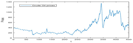
Figure 1.
Time Plot of monthly Crude Oil Prices.
Next, this paper wants to identify the chaotic characteristics of the entire time series from January 1980 to June 2017, and to determine whether the global financial crisis in 2008 will affect the chaotic characteristics of the entire time series, we will consider it in three parts:
(1) The whole time period (January 1980–June 2017)
Firstly, the mutual information function method is used to obtain the delay time = 3, and the embedding dimension m = 7 is determined by Cao method. According to the Wolf algorithm [35], the largest Lyapunov exponent = 0.0617 is greater than 0. It seems that the time series of WTI crude oil prices is chaotic using the chaos recognition theory [33,36,37]. But the largest Lyapunov exponent is close to zero. To evaluate the statistical significance of the largest Lyapunov exponent estimates, we calculate critical values for the empirical distribution of the estimates which is obtained by the Model-based bootstrap method [38]. In statistics, bootstrapping is, involved variables independent at some level, any test or metric that relies on random sampling with replacement. But the repeatability may not be at the level of individual observations, but of groups of them, and there is typically dependence between as well as within groups. This leads to the idea of constructing bootstrap data by taking blocks of some sort from the original observations. One of the methods is Model-based bootstrap, which is analogous to model-based resampling in regression. The idea is to fit a suitable model to the data, to construct residuals from the fitted model, and then to generate new series by incorporating random samples from the residuals into the fitted model. In this paper, The largest Lypunov exponent is a chaotic structure that characterizes time series, while the chaotic structure refers to a deterministic structure inside a time series, rather than an unordered, random structure. Therefore, changing the order of the data in the time series changes the internal structure of the time series, which will have a great influence on the calculated value of the largest Lypunov exponent. This is why we use the model-based bootstrap method. We choose the AR(2) model to fit the observed time series , giving estimated autoregressive coefficient
j = 3, …, n, where represents the residuals. Model-based resampling then proceed by equi-probable sampling with replacement from residuals. We denote the estimated largest Lyapunov exponent , and then re-estimate the largest Lyapunov exponents ( ) using bootstrap samples and construct the empirical distribution for . The result is shown in Figure 2. It is easy to get a confidence interval of (0.0594, 0.0633), when the confidence is . Since the quantiles for the empirical distribution are all larger than the largest Lyapunov exponents, implying that the largest Lyapunov exponents is significantly larger than zero. Therefore, according to the chaos recognition theory, it can be determined that the WTI crude oil prices time series is still chaotic.
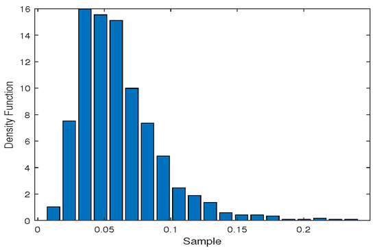
Figure 2.
The histogram of the estimated largest Lyapunov exponent by bootstrap method for the whole period.
(2) Before crisis period (January 1980–June 2008)
We select WTI crude oil monthly prices before crisis period (from January 1980 to June 2008) for a total of 342 data for calculation and analysis.
The mutual information function method we use the mutual information function method to obtain the delay time = 4, and use the Cao method to determine the embedding dimension m = 6. Then the largest Lyapunov exponent = 0.0025 is calculated by Wolf algorithm. Finally, the 95% confidence interval of lambda is (0.0730, 0.0768) using the Model-based bootstrap method, seen in Figure 3. We can conclude that the WTI crude oil prices time series is still chaotic. The calculation process is similar to the whole time period. AR(3) is selected here.
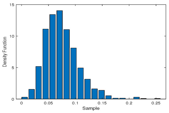
Figure 3.
The histogram of the estimated largest Lyapunov exponent by bootstrap method before crisis period.
(3) After crisis period ( June 2008–June 2017)
A total of 108 monthly WTI crude oil prices after crisis period ( June 2008–June 2017) were selected for calculation and analysis. The mutual information function method we use the mutual information function method to obtain the delay time = 3, and use the Cao method to determine the embedding dimension m = 8. Then the largest Lyapunov exponent = 0.1616 is calculated by Wolf algorithm. Finally, the 95% confidence interval of lambda is (0.1118, 0.1210) using the Model-based bootstrap method, seen in Figure 4. We can conclude that the WTI crude oil prices time series is still chaotic. The calculation process is similar to the whole time period. AR(1) is selected here.
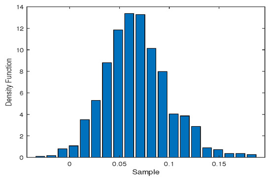
Figure 4.
The histogram of the estimated largest Lyapunov exponent by bootstrap method after crisis period.
As the summary part of this section, the main data of chaos recognition such as lyapunov exponent are listed in a table for easy comparison, as shown in the following Table 1. As can be seen from Table 1, during the whole time period, before and after the crisis, the three time series had chaotic characteristics, indicating that the global financial crisis did not change the chaotic characteristics of the time series.

Table 1.
Chaos test results for the time series of WTI Crude oil price.
3. Prediction Comparison
This paper selects WTI crude oil monthly prices from January 1980 to June 2017 for a total of 450 data for analysis and predicting. For convenience of neural network modeling, we take the first 440 data of the WTI crude oil prices time series as training samples, and the next 10 (or 5) data as prediction test samples.
In the simulation experiment, the original prices and the predicted prices are and respectively, and the experiment uses the error , the Mean Absolute Error (MAE) and the Percentage error (Perr) as the evaluation criteria of the prediction accuracy. The smaller MAE and Perr values are, the more predictive the model is, where MAE and Perr are respectively defined as:
where represents the number of predicted samples.
3.1. Prediction Based on ANN and Chaos
In this subsection, through Chaos and ANN (Artificial Neural Network), we introduce two models to predict the price of WTI crude oil, including RBF-CHAOS model and BP-CHAOS model.
3.1.1. Prediction Based on RBF-CHAOS Model
Moody and Darken [39] proposed a three-layer feed-forward network with a similar structure of multiple layers of forward networks with a single hidden layer, called Radial Basis Function neural network, ie, RBF neural network. RBF neural network is a local approximation network with three typical network structures: input layer, hidden layer and output layer. Take the input number of RBF network as m, which is the embedded dimension mentioned earlier, and the output number as 1, then the RBF neural network mapping , its mathematical expression is
where, is the input vector of the network; is called a radial basis function; represents norm; is the connection weight of the output layer; signifies the center of the radial basis function. In this paper, the gaussian function is adopted as the radial basis function, whose form is
is constant and is called the width value.
We propose a hybrid based RBF neural network model with Chaos (RBF-CHAOS model) and setting the number of neurons in each layer of the RBF neural network is equal to the embedding dimension m of chaotic time series reconstruction phase space. This model is used to analysis the time series of WTI crude oil prices and predicts prices, using the front 440 data of the new time series as training samples, and then forecasting the next 10 months’ prices. Figure 5 is shown. To evaluate the prediction accuracy, MAE with predicted months of 10 and 5 is 1.9521 and 1.1709 respectively, while Perr is 0.29% and 0.1012% respectively.
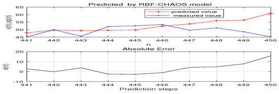
Figure 5.
predicted 10 months’ price by RBF-CHAOS model.
3.1.2. Prediction Based on BP-CHAOS Model
Back Propagation (BP) neural network is a kind of supervised learning neural network with three or more layers of neural networks, including input layer, hidden layer and output layer, using minimum variance learning method [40,41]. Taking the input number of RBF network as m, which also is the embedded dimension mentioned earlier, and the output number as 1, then the RBF neural network mapping The input of each node of its hidden layer is
where, is the connection weight from the input layer to the hidden layer, represents the threshold value of hidden layer node. In this paper, Simoid function is adopted as the transfer function to obtain the output of hidden layer as
Similarly, input and output of output layer nodes are
respectively, where, is the connection weight from the hidden layer to the output layer, and is the threshold of the output layer.
We make use of a hybrid based BP neural network with Chaos (BP-CHAOS model), and setting the number of neurons in the input layer of the neural network is equal to the embedding dimension m of chaotic time series reconstruction phase space. It follows from that using the first 440 data of the WTI crude oil prices time series as training samples, and then forecasting the next 10 months’ prices. Figure 6 presents the simulation results. And through calculation, MAE with predicted months of 10 and 5 is 2.6372 and 1.9903 respectively, while Perr is 0.3318% and 0.1967% respectively.
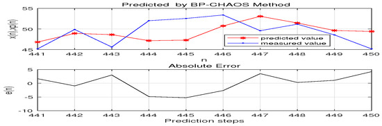
Figure 6.
predicted 10 months’ price by BP-CHAOS model.
Summary In Section 3.1, Chaos theory and ANN technology are used to construct the above two models. The discussion in Section 3.1 is summarized in Table 2 below. Table 2 shows that the prediction accuracy of different models for different months is ranked from high to low as RBF-CHAOS > BP-CHAOS. Meanwhile, MAE value and Perr value of these two models will not exceed 2.7 and 0.35% respectively.
Table 2.
Forecasting with ANN and Chaos.
3.2. Prediction Based on Chaos without ANN
In order to compare the prediction accuracy of the above two models in Section 3.1, a prediction model without ANN technology is constructed based on chaos theory in Section 3.2. Another purpose is to test whether the introduction of ANN technology can improve the prediction accuracy of the model.
We introduce the weighted first-order Local Region (LR-CHAOS) model to predict WTI crude oil prices, which is a local prediction model with Chaos. The main idea of the model is: setting the neighboring point of the center point , , and the distance to is . Setting to be the minimum value of all , and the weight of the point is defined as:
Then the first-order Local Region linear fit is , , where , a and b can be estimated by Weighted Least Squares method [42].
We employ the LR-CHAOS model to predict the WTI crude oil 10 months’ price. The chart is seen in Figure 7. And through calculation, MAE with predicted months of 10 and 5 is 2.0773 and 1.3581 respectively, while Perr is 0.3053% and 0.1758% respectively.
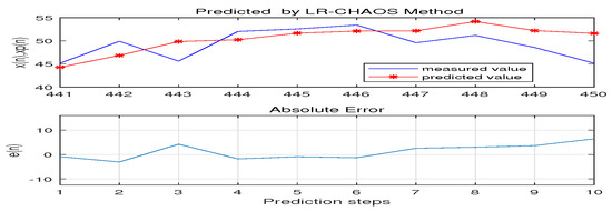
Figure 7.
predicted 10 months’ price by LR-CHAOS model
Summary Combined with Table 2 and Table 3, the prediction accuracy of the three models RBF-CHAOS, BP-CHAOS and LR-CHAOS is ranked from high to low as RBF-CHAOS > LR-CHAOS > BP-CHAOS, which indicates that the prediction model with ANN technology may be better than the model without ANN (RBF-CHAOS > LR-CHAOS), but may also be worse than the model without ANN (LR-CHAOS > BP-CHAOS) on the basis of considering the chaotic characteristics of WTI crude oil price time series. This result also tells us that the introduction of ANN technology in chaos models will not necessarily improve the prediction accuracy of the chaos models.
Table 3.
Forecasting with only Chaos.
3.3. Prediction Based on ANN without Chaos
In order to compare the prediction accuracy of the those three models in Section 3.1 and Section 3.2, this section introduces two prediction models only with ANN, namely, RBF model and BP model. The difference between these two models and those two models in Section 3.1 is that these two models are not based on the chaotic characteristics of time series, while those two models in Section 3.1 are based on the chaotic characteristics of time series. The construction methods of these two models (RBF model and BP model) are shown in Section 3.1 and will not be described here. We are still using the first 440 data of the WTI crude oil price time series to “learn” and predict the next 10 (or 5) months’ price points. Due to the limited space of the paper, the predicted price graphs based on these two models are not presented here. We still list the MAE value and Perr value in a table, and sort these two models according to MAE and Perr value. The smaller the MAE value and Perr value, the higher the corresponding model ordering is, as shown in Table 4.
Table 4.
Forecasting with only ANN.
Summary 1Table 4 shows that the prediction accuracy of these two models for different months is ranked from high to low as RBF > BP. Meanwhile, MAE value and Perr value of these two models will not exceed 3.6 and 0.57% respectively.
Summary 2 The difference between the models in Table 2 and Table 4 is that Table 2 is ANN prediction based on chaotic characteristics of WTI crude oil price time series, while Table 4 is only ANN prediction. The prediction ability of the model was measured from MAE and Perr, and the comparison showed that the prediction ability of the model was ranked from high to low as follows: RBF-CHAOS > RBF, BP-CHAOS > BP, which means the accuracy of the prediction model combining chaos with ANN is higher than that of the ANN model.
Summary 3 When combining Table 3 and Table 4, only chaos prediction is considered in Table 3, while only ANN prediction is considered in Table 4. According to the strength of the prediction ability of the model, the order is: LR-CHAOS > RBF > BP, which indicates that the accuracy of the prediction based only on chaotic features of the WTI crude oil price time series is higher than that based only on ANN.
Summary 4 It can be concluded from Table 2, Table 3 and Table 4 that all prediction models are ranked as RBF-CHAOS > LR-CHAOS > BP-CHAOS > RBF > BP, which indicates that the prediction accuracy of the model based on chaos theory is higher than that of the model without chaos theory. That is to say, the accuracy of the crude oil price prediction model based on chaos theory is better than the ANN prediction model proposed in the existing literature. This shows that our proposing prediction model based on chaos theory is meaningful. Meanwhile, the optimal prediction model among these models is RBF-CHAOS. And it is also found that the accuracy of all models in predicting the price in 5 months is higher than that in 10 months, which means that the accuracy of all models in predicting the short-term price is higher than that in predicting the long-term price.
4. Constructing a New Forecasting Model
We know from the Section 3 that the RBF-CHAOS model has the highest prediction accuracy. In this section, we will construct a new Hybrid model based on the Weight for Percentage error (HWP-CHAOS model) and compare its accuracy with that of the RBF-CHAOS model. The construction method of HWP-CHAOS model is as follows: firstly, the Perr obtained through the above two Chaos+ANN prediction models (RBF-CHAOS model and BP-CHAOS model) are denoted as and respectively, meanwhile, the predicted prices of each model are denoted as and . Next, we convert Perr to the weight of the corresponding model, as follows:
where, is the weight given to model RBF-CHAOS, the weight given to model BP-CHAOS is denoted as . It follows from that the predicted WTI crude oil price
We know that the higher the Perr value is, the worse the prediction ability of the corresponding model will be. Therefore the implication of HWP-CHAOS model is that the greater the value of Perr, the less weight is assigned to the corresponding model forecasting price, which provides a new perspective for crude oil price forecast. And through calculation, MAE with predicted months of 10 and 5 is 1.7502 and 0.9581 respectively, while Perr is 0.2007% and 0.0958% respectively (see Figure 8).
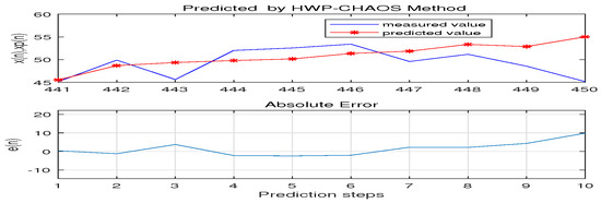
Figure 8.
Predicted 10 months’price by HWP-CHAOS model.
Summary In order to compare the prediction accuracy of the above three type models, (in fact, the RBF-CHAOS model can only be compared, because the prediction accuracy of the RBF-CHAOS model is the highest among the five models discussed in the Section 3), the MAE and Perr values of the RBF-CHAOS model and HWP-CHAOS model are listed in the following Table 5. We acquaint that the accuracy of the HWP-CHAOS model is higher than that of the RBF-CHAOS model, which means that the new prediction model can better predict WTI crude oil prices.
Table 5.
Compared to RBF-CHAOS and HWP-CHAOS.
5. Conclusions
This paper first analyzes the chaotic characteristics of the time series of WTI crude oil price, which is the basis of building an appropriate model to predict. When using the largest lyapunov exponent to determine the chaotic characteristics of time series, we used bootstrap method to test the robustness of the largest lyapunov exponent, which effectively overcame the misjudgment of chaos identification. We not only made chaotic judgment on the entire time series from January 1980 to June 2017, but also made chaotic judgment on the two time series before and after the financial crisis (July 2008). We find that financial crises do not change the chaotic character of time series. Then, we construct three models (HWP-CHAOS model, RBF-CHAOS model and BP-CHAOS model) that contain both Chaos and ANN to predict the price of WTI crude oil. In order to test the accuracy of these three prediction models, two types of models are constructed respectively, one type is the prediction model (LR-CHAOS model) which has only Chaos but not ANN, and the other type is the prediction model (RBF model and BP model) which has only ANN but not Chaos. Through the comparative analysis of these three type models, we found the following points:
- (1)
- Our findings suggest that WTI crude oil price series is not Martingale (i.e. it is predictable) and follows a non-linear trend. So, the efficient market hypothesis is not valid in this case;
- (2)
- the prediction accuracy of the model based on Chaos (HWP-CHAOS model, RBF-CHAOS model, BP-CHAOS model and LR-CHAOS model) is higher than that of the model using ANN but without chaos (HWP model, RBF model and BP model);
- (3)
- the prediction accuracy of ANN+Chaos-type model (HWP-CHAOS model, RBF-CHAOS model and BP-CHAOS model) is not necessarily higher than the only Chaos-type model (LR-CHAOS model);
- (4)
- the best prediction model is HWP-CHAOS model among the models discussed in this paper;
- (5)
- the accuracy of all models in predicting the price in 5 months is higher than that in 10 months.
Author Contributions
Conceptualization, T.Y. and Y.W.; Data curation, T.Y.; Formal analysis, T.Y.; Investigation, T.Y.; Methodology, T.Y. and Y.W.; Project administration, Y.W.; Software, T.Y.; Supervision, Y.W.; Writing—original draft, T.Y.; Writing—review & editing, T.Y.
Funding
This research was funded by Key Laboratory of Mathematical Economics and Quantitative Finance (Peking University), Ministry of Education.
Acknowledgments
The authors mainly acknowledge the support of Key Laboratory of Mathematical Economics and Quantitative Finance (Peking University), Ministry of Education.
Conflicts of Interest
The authors declare no conflict of interest.
References
- Alvarez-Ramirez, J.; Soriano, A.; Cisneros, M.; Suarez, R. Symmetry/anti-symmetry phase transitions in crude oil markets. Physica A 2003, 322, 583–596. [Google Scholar] [CrossRef]
- Verleger, P.K. Adjusting to Volatile Energy Prices; Institute for International Economics: Washington, DC, USA, 1993. [Google Scholar]
- Sivakumar, B. Chaos theory in hydrology: Important issues and interpretations. J. Hydrol. 2000, 227, 1–20. [Google Scholar] [CrossRef]
- Sivakumar, B. Chaos theory in geophysics: Past, present and future. Chaos Solitons Fractals 2004, 19, 441–462. [Google Scholar] [CrossRef]
- Rudnicki, R. Chaos for some infinite-dimensional dynamical systems. Math. Methods Appl. Sci. 2010, 27, 723–738. [Google Scholar] [CrossRef]
- Man, K.S. Long memory time series and short term forecasts. Int. J. Forecast. 2003, 19, 477–491. [Google Scholar] [CrossRef]
- Lahmiri, S. On fractality and chaos in Moroccan family business stock returns and volatility. Phys. A Stat. Mech. Appl. 2017, 473, 29–39. [Google Scholar] [CrossRef]
- Kazem, A.; Sharifi, E.; Hussain, F.K.; Saberi, M.; Hussain, O.K. Support vector regression with chaos-based firefly algorithm for stock market price forecasting. Appl. Soft Comput. J. 2013, 13, 947–958. [Google Scholar] [CrossRef]
- Hanias, M.P.; Ozun, A.; Curtis, P.G. A chaos analysis for Greek and Turkish equity markets. EuroMed J. Bus. 2010, 5, 101–118. [Google Scholar]
- Pandey, V.; Kohers, T.; Kohers, G. Deterministic nonlinearity in the stock returns of major European equity markets and the United States. Financ. Rev. 2010, 33, 45–64. [Google Scholar] [CrossRef]
- Chen, P. Empirical and theoretical evidence of economic chaos. Syst. Dyn. Rev. 1988, 4, 81–108. [Google Scholar] [CrossRef]
- Chwee, V. Chaos in natural gas futures. Energy J. 1998, 19, 149–164. [Google Scholar] [CrossRef]
- Serletis, A.; Gogas, P. The North American natural gas liquids markets are chaotic. Energy J. 1999, 20, 83–103. [Google Scholar] [CrossRef]
- Adrangi, B.; Chatrath, C. Chaos in oil prices? Evidence from futures market. Energy Econ. 2001, 23, 405–425. [Google Scholar] [CrossRef]
- Gu, R.; Chen, H.; Wang, Y. Multifractal analysis on international crude oil markets based on the multifractal detrended fluctuation analysis. Physica A 2010, 389, 2805–2815. [Google Scholar] [CrossRef]
- Cajueiro, D.O.; Tabak, B.M. Testing for long-range dependence in the Brazilian term structure of interest rates. Chaos Solitons Fractals 2009, 40, 1559–1573. [Google Scholar] [CrossRef]
- Sensoy, A. Effects of monetary policy on the long memory in interest rates: Evidence from an emerging market. Chaos Solitons Fractals 2013, 57, 85–88. [Google Scholar] [CrossRef]
- Lahmiri, S. Long memory in international financial markets trends and short movements during 2008 financial crisis based on variational model decomposition and detrended fluctuation analysis. Physica A 2015, 437, 130–138. [Google Scholar] [CrossRef]
- Lahmiri, S. Investigating long-range dependence in American treasury bills variations and volatilities during stable and unstable periods. Fractals 2016, 24, 1650025. [Google Scholar] [CrossRef]
- Morales, R.; Di Matteo, T.; Gramatica, R.; Aste, T. Dynamical generalized Hurst exponent as a tool to monitor unstable periods in financial time series. Physica A 2012, 391, 3180–3189. [Google Scholar] [CrossRef]
- Komijani, A.; Naderi, E.; Gandali Alikhani, N. A Hybrid Approach for Forecasting of Oil Prices Volatility. MPRA Pap. 2013, 38, 323–340. [Google Scholar] [CrossRef]
- Abramson, B.; Finizza, A. Using belief networks to forecast oil prices. Int. J. Forecast. 1991, 7, 299–315. [Google Scholar] [CrossRef]
- Kaboudan, M.A. Compumetric forecasting of crude oil prices. In Proceedings of the IEEE Congress on Evolutionary Computation, Seoul, Korea, 27–30 May 2001; pp. 283–287. [Google Scholar]
- Mirmirani, S.; Li, H.C. A comparison of VAR and neural networks with genetic algorithm in forecasting price of oil. Adv. Econom. 2004, 19, 203–223. [Google Scholar]
- Zhang, J.L.; Zhang, Y.J.; Zhang, L. A novel hybrid method for crude oil price forecasting. Energy Econ. 2015, 49, 649–659. [Google Scholar] [CrossRef]
- Shambora, W.E.; Rossiter, R. Are there exploitable inefficiencies in the futures market for oil? Energy Econ. 2007, 29, 18–27. [Google Scholar] [CrossRef]
- Yu, L.; Lai, K.K.; Wang, S.Y.; He, K.J. Oil price forecasting with an EMD-based multiscale neural network learning paradigm. Lect. Notes Comput. Sci. 2007, 4489, 925–932. [Google Scholar]
- Moshiri, S.; Foroutan, F. Forecasting nonlinear crude oil futures prices. Energy J. 2006, 27, 81–95. [Google Scholar] [CrossRef]
- Takens, F. Detecting strange attractors in turbulence. In Dynamical Systems and Turbulence; Rand, D., Young, V., Eds.; Lecture Notes in Mathematics; Springer: Berlin, Germany, 1980; Volume 898, pp. 266–382. [Google Scholar]
- Takens, F. Distinguishing deterministic and random systems. In Nonlinear Dynamics and Turbulence; Borenblatt, G., Iooss, G., Joseph, D., Eds.; Pittman: Boston, MA, USA, 1983; pp. 315–333. [Google Scholar]
- Wang, J.Z.; Wang, J.J.; Zhang, Z.G.; Guo, S.P. Forecasting stock indices with back propagation neural network. Expert Syst. Appl. 2011, 38, 14346–14355. [Google Scholar] [CrossRef]
- Kim, H.S.; Eykholt, R.; Salas, J.D. Delay time window and plateau onset of the correlation dimension for small data sets. Phys. Rev. E 1998, 58, 5676–5682. [Google Scholar] [CrossRef]
- Rosenstein, M.T.; Collins, J.J.; Luca, C.J.D. A practical method for calculating largest Lyapunov exponents from small data sets. Phys. D-Nonlinear Phenom. 1993, 65, 117–134. [Google Scholar] [CrossRef]
- Fraser, A.M.; Swinney, H.L. Independent coordinates for strange attractors from mutual Information. Phys. Rev. A 1986, 32, 1134. [Google Scholar] [CrossRef]
- Wales, D.J. Calculating the rate of loss of information from chaotic time series by forecasting. Nature 1991, 350, 485–488. [Google Scholar] [CrossRef]
- Wolf, A.; Swift, J.B.; Swinney, H.L.; Vastano, J.A. Determining Lyapunov exponents from a time series. Phys. D Nonlinear Phenom. 1985, 16, 285–317. [Google Scholar] [CrossRef]
- Zhang, X.; Xu, J. Face recognition based on the chaos theory and support vector machine. Chin. High Technol. Lett. 2009, 19, 494–500. [Google Scholar]
- Davison, A.C.; Hinkley, D.V. Bootstrap Methods and Their Application; Cambridge University Press: Cambridge, UK, 1997. [Google Scholar]
- Moody, J.; Darken, C.J. Fast learning in networks of locally-tuned processing units. Neural Comput. 1989, 1, 281–294. [Google Scholar] [CrossRef]
- Rumelhart, D.E.; Hinton, G.E.; Williams, R.J. Learning Internal Rep-Resentations by Error Propagation in Parallel Distributed Processing; MIT Press: Cambridge, MA, USA, 1986; pp. 318–362. [Google Scholar]
- Yang, S.; Tseng, C.S. An orthogonal neural network for function approximation. IEEE Tran. Syst. Man Cybern. Part B 1996, 26, 779–785. [Google Scholar] [CrossRef] [PubMed]
- Zhang, Q.Y.; Pan, L.; Zi, X.C. A Shared Congestion Detection Technique Based on Weighted First Order Local-Region Method. J. Shanghai Jiaotong Univ. 2010, 44, 277–286. [Google Scholar]
© 2019 by the authors. Licensee MDPI, Basel, Switzerland. This article is an open access article distributed under the terms and conditions of the Creative Commons Attribution (CC BY) license (http://creativecommons.org/licenses/by/4.0/).